A new approach to characterize emission contributions from area sources during optical remote sensing technique testing

Abstract

In the method termed “Other Test Method-10,” the U.S. Environmental Protection Agency has proposed a method to quantify emissions from nonpoint sources by the use of vertical radial plume mapping (VRPM) technique. The surface area of the emitting source and the degree to which the different zones of the emitting source are contributing to the VRPM computed emissions are often unknown. The objective of this study was to investigate and present an approach to quantify the unknown emitting surface area that is contributing to VRPM measured emissions. Currently a preexisting model known as the “multiple linear regression model,” which is described in Thoma et al. (2009), is used for quantifying the unknown surface area.

The method investigated and presented in this paper utilized tracer tests to collect data and develop a model much like that described in Thoma et al. (2009). However, unlike the study used for development of the multiple linear regression model, this study is considered a very limited study due to the low number of pollutant releases performed (seven total releases). It was found through this limited study that the location of an emitting source impacts VRPM computed emissions exponentially, rather than linearly (i.e., the impact that an emitting source has on VRPM measurements decreases exponentially with increasing distances between the emitting source and the VRPM plane). The data from the field tracer tests were used to suggest a multiple exponential regression model. The findings of this study, however, are based on a very small number of tracer tests. More tracer tests performed during all types of climatic conditions, terrain conditions, and different emissions geometries are still needed to better understand the variation of capture efficiency with emitting source location. This study provides a step toward such an objective.

Implications

The findings of this study will aid in the advancement of the VRPM technique. In particular, the contribution of this study is to propose a slight improvement in how the area contributing to flux is determined during VRPM campaigns. This will reduce some of the technique's inherent uncertainties when it is employed to estimate emissions from an area source under nonideal conditions.

Background

The ability for a technique to accurately measure pollutant emissions from nonpoint sources will provide a more reliable emission inventory, which will allow for those responsible for their emissions to acknowledge and prevent further emissions. Together, acknowledgment of emissions and the desire to reduce emissions for energy producing purposes can ultimately result in a reduced greenhouse gas inventory. However, in order to provide estimates of emissions, an economical technique must be used to accurately measure pollutant emission from area sources.

One of the more notable nonpoint source measurement approaches is the use of an optical remote sensing technique known as the vertical radial plume mapping (VRPM) method (U.S. Environmental Protection Agency [EPA], 2004, 2006, 2007). The VRPM method is used to obtain a mass-equivalent plume map, which is combined with wind speed and wind direction to obtain a desired pollutant flow rate (mass per time) that crosses the optical beams that are arranged in a vertical array.

As shown in the graphical illustration of the VRPM setup (Figure 1), there are three retro-reflectors at ground level, the first one at one-third of the distance to the final retro-reflector and the second at two-thirds of the distance to the final retro-reflector. Two more retro-reflectors are used above the ground height. The retro-reflectors at ground level ranged from approximately 1 to 3 m above ground surface. Typically the two retro-reflectors above the ground level are strapped to a scissor jack at mid-height (approximately at 5 m above ground surface) of the jack and at full height (approximately 10 m above ground surface) of the jack.

Figure 1. Schematic sketch of Vertical Radial Plume Mapping (VRPM) setup.

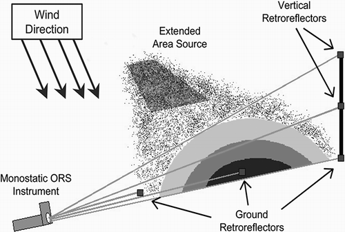
The VRPM configuration consists of the aforementioned five retro-reflectors that together create the measurement plane. By utilizing three retro-reflectors on the ground surface and two above the ground surface, the optical remote sensing technique is capable of obtaining the location on the plane that results in the highest pollutant concentration of the plume that is actively crossing the optical beams. Thereafter, the technique constructs the pollutant map by interpolating the computed emissions, and connecting the interpolated points of equivalent concentrations.

Two anemometers are utilized to determine wind direction and velocity at 2 and 10 m above ground surface. Generally, one of the anemometers is placed near the scissor jack at the full extent of the VRPM plane, and the second is generally placed near the optical remote sensing device. The product of the mass-equivalent concentration map and the wind speed normal to the measurement plane are integrated across the plane to calculate the mass flow through the plane in grams per second. For typical wind conditions, the VRPM configuration was reported to have an accuracy within 11% (Thoma et al., 2005). However, VRPM configuration can significantly underestimate gas mass flux under unstable atmospheric conditions (Hashmonay et al., 2001).

The VRPM technique utilizes a computation algorithm to perform a two-stage smooth basis function minimization plume reconstruction (Drescher et al., 1996, 1997). A one-dimensional smooth basis function is initially applied in order to reconstruct the smoothed ground level and crosswind concentration profile. A bivariate Gaussian function is then fitted to the measured path integrated concentration values at ground level. A two-dimensional smooth basis function minimization is then used to reconstruct the smoothed mass equivalent concentration map (Hashmonay et al., 2008). Further information regarding methods and calculations used in the VRPM methodology can be found in the U.S. EPA 2006 OTM-10 Optical Remote Sensing for Emission Characterization From Non-Point Sources, which is the U.S. EPA's standard VRPM manual.

Optical remote sensing techniques, such as the VRPM, have been found to work well under the following conditions: when the emitting source's location and boundaries are known; when the emitting source is small in comparison to the VRPM plane length; when the optical remote sensing instruments are closely spaced apart; and when the wind is constantly blowing the plume in the direction perpendicular to the optical beam paths. However, many uncertainties associated with the VRPM technique remain (Abichou et al., 2010). One of the greatest concerns associated with the VRPM technique is having insufficient knowledge on how much of the emitting source's area is actually being accounted for in the VRPM measurements, known as the area contributing to flux (ACF). Thoma et al. (2009) introduced the term ACF and defined it as the area of the emitting source that is contributing to VRPM-measured mass flow rate. It also can be defined as the zones of the emitting source where the capture efficiency is greater than zero. The term “capture efficiency” was defined as the VRPM-measured or estimated mass flow rate divided by the released mass flow rate. To compute the emission per unit area, an estimate of ACF is essential.

U.S. EPA-Waste Management, Inc. field tests were conducted to establish capture efficiencies for various upwind locations, and to determine ACF for use with optical remote sensing method for future applications (Goldsmith et al., 2008; Green et al., 2009). Results from these tracer tests were analyzed using a multiple linear regression model to provide estimates of ACF. The use of the multiple linear regression model is explained in Thoma et al. (2009). Thoma et al. (2009) utilized wind adjusted release distances (WARD) to develop capture efficiencies for upwind release locations. The WARD is the distance from the release location to the measurement plane after considering variable wind directions (Thoma et al., 2009). The linear regression model has the ability to compute theoretical capture efficiencies for various WARD, which results in the ability to calculate an estimate of the ACF. Parameters to compute the ACF using the multiple linear regression model are as follows: VRPM plane length, wind speed, wind direction, and release distances. An alternative approach to the multiple linear regression model is proposed in this study. This alternative approach is a multiple exponential regression model.

Methods

Field tracer tests

Tracer tests were performed by our research team on a non-pollutant-emitting site in Louisville, KY. Background concentration readings were performed for a minimum of 30 min before each tracer gas release. The background concentrations were deducted from computed concentrations during the tracer test.

The tracer tests were performed on January 8, 2009, and January 9, 2009. The testing utilized 18 acres of the site. The morning of Day 1 was the coldest at 0°C and the morning of Day 2 was around 3.3°C. Day 1 and Day 2 were both considered sunny with a prevailing wind direction of approximately 300° and 21° from the north, respectively. Although temperature measurements were not conducted throughout the two days, the assumed incoming solar radiation (sunny) and the assumed prevailing wind speeds and directions are consistent with the climatic data obtained from the Louisville International Airport weather station (less than 10 miles from the testing location), for the time period when the VRPM testing was performed.

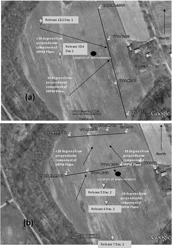
VRPM measurements were conducted during the hours of 9:40 a.m. to 4:40 p.m. and 11:40 a.m. to 4:10 p.m. on Day 1 and Day 2, respectively. Wind speeds ranged from 1.6 m per second to approximately 3.9 m per second during the 2-day study. Figures 2a and 2b present the site location and the VRPM configurations for both days of the experiment. In Figure 2, the “TDL” stands for “tunable diode laser” (which is the optical remote sensing device used in the study), “M” stands for “mirror,” “R” stands for “release,” and “D” stands for “day” (e.g., “TDL3-M2-D1” found in Figure 2a represents the location of mirror 2 on Day 1 for the VRPM plane created by TDL 3).

Figure 2. (a) Day one; (b) Day two VRPM configuration with release locations.

The gas released consisted of 99.99% technical grade methane. Releases from point sources and area sources were conducted in the case study. Calibrated mass flow controllers were used to accurately control and measure the amount of methane released from the compressed gas cylinder throughout the entire release time duration. In addition to the calibrated mass flow controllers, the compressed gas cylinders were weighed before and after the releases to ensure the release data provided by the calibrated mass flow controllers were valid.

Through the two days, seven releases were performed in total, four releases the first day and three releases the second day. Three of the seven releases (releases 1, 2, and 3) were considered area releases and the remaining four releases (releases 4, 5, 6, and 7) were considered point releases.

In order to simulate an area source in the field, mats were constructed using polyvinyl chloride (PVC) pipes and a thin layer of insulation covering the pipes for diffusion purposes. Holes were drilled in relatively evenly spaced intervals along the four sides of the PVC piping. The PVC pipes were attached using 90° corner PVC “connectors.” Three mats were used, placed one on top of the next, and each mat was connected to a separate methane cylinder. All three cylinders started to release the methane simultaneously to achieve a larger flow rate. The mat dimensions were square-shaped with each side measuring approximately 3.048 m in length. Therefore the total area of emissions was 9.29 m². All releases were classified as surface releases.

Table 1 shows the release locations in comparison to the three VRPM planes used during the two-day period, release type (i.e., point or area source), averaged emission rates for each release time period, and the total plane length used during the release. The “X” in Table 1 represents the length of an imaginary line that runs from the release location perpendicular to the VRPM plane. The “Y” is the distance from the TDL to the point where the imaginary perpendicular line created by the “X” crosses the VRPM plane.

Table 1. Field release locations and release types

Day	TDL	Release #	Release Type (area or point)	Release Amount (g/sec)	X(m)	Y(m)	Plane Length (m)
1	3	1	Area	1.73	170	306	318
		2	Area	6.53	170	306
		3	Area	6.65	140	207
		4	Point	5.96	140	207
2	1	5	Point	5.89	155	90	165
		6	Point	5.99	205	90
		7	Point	6.88	305	85
2	3	5	Point	5.89	50	120	239
		6	Point	5.99	100	120
		7	Point	6.88	200	112

Using recorded meteorological data, Day 1 releases (1 through 4, Figure 2 a) had a predominant wind direction of 313, 313, 307, and 307° from north respectively. Day 2 releases (5, 6, and 7, Figure 2 b) had a predominant wind direction of 234, 217, and 198° from north respectively.

Field vertical radial plume mapping

The tunable diode laser employed in this VRPM study is a computer-controlled device that sequentially cycles through each retro-reflector automatically. The flux (g/sec) results were calculated by commercial software (Arcadis, 2007) using the equations described in U.S. EPA OTM 10 (2006).

The field tunable diode laser held stationary on each retro-reflector for anywhere between 20 and 60 sec. The time delay is used for the flux calculator to compute the path-integrated concentrations for each beam path. The tunable diode laser used in this study was a GasFinder 2.0, manufactured by Boreal Laser, Spruce Grove, Alberta, Canada. Wind speeds and directions were constantly measured during the study using calibrated R. M. Young meteorological heads, located at approximately 2 m and 10 m above the ground surface.

In order to provide additional data points, two VRPM planes were configured on Day 2. The two data sets obtained by the two planes on Day 2 were not compared to one another, but analyzed separately. Therefore, throughout the study, ina total three planes were used and analyzed separately, resulting in three data sets, and theoretically 10 releases (there were technically only seven releases, but since two planes were used on the second day, the three releases on Day 2 resulted in six measured releases).

On Day 1, a VRPM plane length of 318 m was used with an approximate 345° from north VRPM orientation. On Day 2, VRPM plane lengths for TDL-1 and TDL-3 were 237 and 170 m respectively. Orientations for the two VRPM planes on Day 2 were approximately 260 and 270° from north, respectively. The VRPM configuration for this study was set up in accordance with the specifications defined in the U.S. EPA Test Method-10 (OTM-10).

VRPM plane orientations were carefully considered when drawing up the initial plans. The VRPM plane was chosen to be as relatively close to the perpendicular of the prevailing wind direction as possible. On Day 2, the two planes' orientations differed slightly from each other to help create a larger range of acceptable wind directions. Based on OTM-10 methodology, as presented in the U.S.EPA (2006) manual, a wind direction range of plus/minus 30° from perpendicular to the VRPM plane is considered acceptable. Capture efficiencies were computed by dividing the mass flow of methane crossing the VRPM plane by the mass flow of methane being emitted from the assigned source.

Results and Discussions

As stated earlier, capture efficiency is defined as the ratio of the mass flow of gas estimated by the VRPM divided by the flow of methane released from the compressed gas cylinders from the tracer tests. Capture efficiencies were calculated for time periods when wind directions were within the appropriate ±30° range, in accordance with the U.S. EPA “Other Test Method-10” manual (U.S.EPA, 2006).

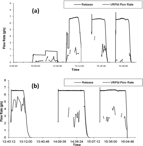
In addition to the ±30° wind angle criteria, time periods of selected data were chosen so that a steady state condition is likely to exist between the VRPM measurement and the emitting gas cylinders. Figure 3 illustrates the time delay between the actual release time and the VRPM measurement time. Figures 3a and 3b represent the release flow mass in comparison to the VRPM measurements for the two days when testing was performed. By accounting for the time delay, a steady-state condition is more likely to occur. After reviewing Figure 3, certain VRPM readings were excluded from the data sets based on the aforementioned time delay. These readings were the first few measurements and the final few measurements. Judgment was used for determining which data points to exclude based on perceived variability in results due to the time delay between the compressed gas cylinder operations and VRPM plane measurements. The measurements taken when wind directions exceeded the ±30° range were then manually removed per OTM-10 requirements. This requirement is one of the main disadvantages of the VRPM method because after the initial setup of the VRPM plane, wind directions may vary beyond the acceptable limitations, which in turn will greatly reduce VRPM measurement accuracy.

Figure 3. (a) Day one; (b) Day two comparison of release and capture.

After removing some of the data from Figure 3 (due to the time delay and unacceptable wind direction described above), the remaining data were converted to capture efficiency, as previously defined, and plotted versus WARD (defined earlier) on Figure 4. The “open diamond” data points in Figure 4 represent the actual field-measured capture efficiencies. The dashed exponential line presented in Figure 4 is a best-fit line applied to the actual field. The multiple linear regression method described in Thoma et al. (2009) was used to compute theoretical capture efficiencies using actual wind speeds along with corresponding WARD data. These theoretical capture efficiencies are presented on Figure 4 with “closed triangles.” As expected and indicated by the actual field data, the capture efficiency decreases with increasing WARD. Therefore, some form of a regression model is required to describe the variation of capture efficiency with WARD. Finally, as observed by Thoma et al. (2009), the data show tremendous scatter and variability of capture efficiency at a constant WARD.

Figure 4. Capture efficiency vs. WARD from all tracer tests, along with Multiple Linear Regression (MLR) Model and Multiple Exponential Regression (MER) Model.

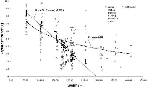
It can also be seen from Figure 4 that, for release locations far away from the VRPM plane (WARD > 200 m), the multiple linear regression model underestimates the contributions from these locations. A multiple exponential regression model was found to better represent the data points with WARD larger than 250 m. The multiple linear regression model assigns a capture efficiency value of zero to the contributions of sources that are further than 250 m of WARD. An exponential function, however, would be capable of estimating positive values more aligned with the actual data points, even for distances greater than 250 m of WARD. It is worth noting, though, that the data reported by Thoma et al. (2009) was obtained with WARD distances less than 250 m. If we look at the portion of our data that corresponds to WARD distances in the same range of the WARD measured in Thoma et al. (2009), a similar linear regression can be obtained. However, when we add the portion of our data with WARD from 250 to 400 m, these additional data seem to render an exponential fit better than a linear fit.

Thoma et al. (2009) was used to compute capture efficiencies for the maximum and minimum wind speeds recorded in the field during the tracer tests. These theoretical capture efficiencies were plotted for small incremental increases in WARD values. The dark lines labeled “1.6 m/sec” and “3.9 m/sec” in Figure 5 represent the theoretical data points computed using the multiple linear regression model for the respective WARD value on the x-axis for the two wind speeds. By simply counting the actual field measured data points that fall within the linear regression model's boundaries in Figure 5 (between the two lines obtained using the two limits of wind speeds), 64% of the tracer test data points fall between the two lines corresponding to the minimum and maximum encountered wind speeds. Figure 5 also shows that only 7% of the data points at WARD values larger than 230 m fall within the range associated with the two limits of encountered wind speeds. Furthermore, for the wind speeds encountered during the two-day study, the multiple linear regression model predicts capture efficiencies of zero for all WARD values greater than 330 m. The field data, however, show measured capture efficiencies up to 43% at 400 m of WARD. Therefore, the multiple linear regression model underestimates, neglects, or disregards contributions from far-away sources (+250 m for this study). For many applications, however, the emitting source can be extensively large so that the contribution of further portions of the source cannot be neglected. The statements just provided are accurate for the data sets analyzed in this study, which only include emission sources on a gently sloping but level terrain. The alternative approach, presented herein, to the multiple linear regression model is a multiple exponential regression model, as shown in Figure 6. The same procedures used to compute the theoretical capture efficiencies with the multiple linear regression model were used to compute theoretical capture efficiencies with the multiple exponential regression model ( eq 1). Again, the dark lines plotted in Figure 6 represent the theoretical capture efficiencies computed for gradual incremental increases in WARD values. The remaining data points represented in Figure 6 are the actual field measured capture efficiencies, which are the same as the ones presented in Figure 5. The following equation represents the multiple exponential regression model:

Figure 5. Multiple Linear Regression (MLR) Model for wind speeds 1.6 and 3.9 m/sec.

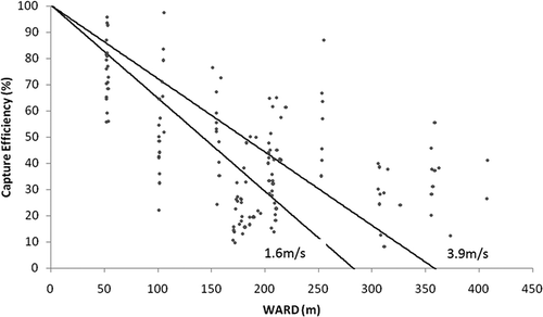
Figure 6. Multiple Exponential Regression (MER) Model for wind speeds 1.6 and 3.9 m/sec.

1

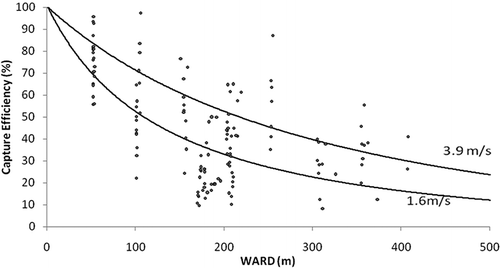
where CE is the capture efficiency, WARD is the wind adjusted release distance, and WS is the wind speed. When using the multiple exponential regression model, 81% of the observed data points plots within the range of the maximum and minimum encountered wind speeds, but more importantly, 64% of the recorded VRPM data at WARD values greater than 230 m are also within the two lines describing the limits of the exponential regression model.

Trend lines and “goodness-of-fit” evaluations were not performed due to the fact that the data points plotted in Figures 5 and 6 represent capture efficiencies for all encountered wind speeds. If the plotted data were to have been separated into different wind speed categories, then trend lines could have been used. Therefore, the solid lines indicated on Figures 5 and 6 represent the capture efficiencies that the multiple linear regression model (Figure 5) and the multiple exponential regression model (Figure 6) predicted using the maximum and minimum encountered wind speeds. If a data point falls within these two lines, then for a particular wind speed between 1.6 m/sec and 3.9 m/sec, the model(s) will be able to predict the actual VRPM capture efficiency for that particular WARD.

As an example, for an initial source boundary distance of 0 m, a final source boundary distance of 325 m, a VRPM plane length of 150 m, and a wind speed of 3 m/sec, the multiple linear regression model produced an ACF of 24,375 m², while the multiple exponential regression model produced an ACF of 32,127 m² for the same wind speed. Although it is the author's belief that the multiple exponential regression model is more representative than the multiple linear regression model, the drawback is that the multiple linear regression model is a more conservative approach. The smaller the ACF is, the greater the emission flux is from the emitting source.

Conclusions

Site-specific determination of the ACF could be computed by simply verifying the current wind speed during VRPM testing and then obtaining the exponential function that correlates with that specific wind speed. Of course, in order to better correlate ACF with wind speed, one would need to perform more tracer testing during a wide range of wind speeds. The use of the exponential regression model to estimate an ACF may allow for a reduction in the level of uncertainty associated with the VRPM method. However, regardless of which regression model is used, or how accurate the model is at estimating the ACF, significant uncertainties (as described in Abichou et al. [2010]) are inherent in the current state of the VRPM method. Therefore, regardless of the accuracy of the model used, the VRPM technique in its current state will still exhibit uncertainties in actual emission flux readings.

Although the use of the VRPM technique may not be appropriate for use as a means of accurately assessing emissions from an area source in its current condition, if each uncertainty is individually studied and improved upon (such as the ACF), the VRPM technique may one day be used to accurately quantify emissions from area sources. The findings of this study, however, are based on a very small number of tracer tests. More tracer tests performed during all types of climatic conditions, terrain conditions, and different emissions geometries are still needed to better understand the variation of capture efficiency with emitting source location. This study provides a step toward such an objective.

References

- Abichou , T. , Clark , J. , Tan , S. , Chanton , J. , Hater , G. , Green , R. , Goldsmith , D. , Barlaz , M. and Swan , N. 2010 . Uncertainties associated with the use of optical remote sensing technique to estimate surface emissions in landfill applications . J. Air Waste Manage. Assoc. , 60 : 460 – 470 . doi: 10.3155/1047-3289.60.4.460
- Arcadis , Inc . 2007 . ARCADIS Flux Calculator Software for VRPM Analysis. Durham, NC
- Drescher , A.C. , Gadgil , A.J. , Price , P.N. and Nazaroff , W.W. 1996 . Novel approaches for tomographic reconstruction of gas concentration and distributions in air: Use of smooth basis functions and simulated annealing . Atmos. Environ. , 30 : 929 – 940 . doi: 10.1016/1352-2310(95)00295-2
- Drescher , A.C. , Park , D.Y. , Yost , M.G. , Gadgil , A.J. , Levine , S.P. and Nazaroff , W.W. 1997 . Stationary and time dependent tracer-gas concentrations measured by OP-FTIR remote sensing and SBFM computed tomography . Atmos. Environ. , 31 : 727 – 740 . doi: 10.1016/S1352-2310(96)00221-X
- Gifford , F.A. 1960 . “ Atmospheric dispersion calculations using the generalized Gaussian plume model ” . In Nuclear Safety 56 – 59 .
- Goldsmith , C.D. , Hater , G. , Green , R. , Abichou , T. , Barlaz , M. and Chanton , J. 2008 . “ Comparison of optical remote sensing with static chambers for quantification of landfill methane emission. Paper presented at Global Waste Management Symposium ” . In Copper Mountain, CO, September
- Green , R.B. , Hater , G. , Goldsmith , D. , Chanton , J. , Swan , N. and Abichou , T. March 2009 . “ Estimates of methane emissions from three California landfills using two measurement approaches ” . In Presented at the A&WMA 1st International Greenhouse Gas Measurement Symposium March , San Francisco , CA
- Hashmonay , R.A. , Natschke , D.F. , Wagner , K. , Harris , D.B. , Thompson , E.L. and Yost , M.G. 2001 . Field evaluation of a method for estimating gaseous fluxes from area sources using open-path Fourier transform infrared . Environ. Sci. Technol. , 35 : 2309 – 2313 . doi: 10.1021/es0017108
- Hashmonay , R.A. , Varma , R.M. , Modrak , T.M. , Kagann , R.H. , Segall , R.R. and Sullivan , P.D. 2008 . Advanced Environmental Monitoring. Dordrecht 21 – 36 . Springer , , The Netherlands
- Thoma , E.D. , Shores , R.C. , Thompson , E.L. , Harris , D.B. , Thorneloe , S.A. , Varma , R. , Hashmonay , R.A. , Modrak , M.T. , Natschke , D.F. and Gamble , H.A. 2005 . Open path tunable diode laser absorption spectroscopy for acquisition of fugitive emission flux data . J. Air Waste Manage. Assoc. , 55 : 658 – 668 . doi: 10.1080/10473289.2005.10464654
- Thoma , E.R. , Green , R. , Hater , G. , Goldsmith , C. , Swan , N. , Chase , M. and Hashmonay , R. 2010 . Development of EPA OTM-10 for landfill applications . J. Environ. Eng. , 136 : 769 – 776 .
- U.S. Environmental Protection Agency. 2004. Measurements of Fugitive Emissions at Region I Landfill. EPA-600/R-04-001. U.S. United States Environmental Protection Agency, Washington, DC http://www.epa.gov/nrmrl/pubs/600r04001/600r04001.pdf (http://www.epa.gov/nrmrl/pubs/600r04001/600r04001.pdf)
- U.S. Environmental Protection Agency . 2006 . “ Test Method (OTM-10): Optical Remote Sensing for Emission Characterization from Non-Point Sources ” . In Research Triangle Park, NC: U.S. Environmental Protection Agency , Technology Transfer Network Emission Measurement Center .
- U.S. Environmental Protection Agency . 2007 . “ Evaluation of Fugitive Emissions Using Ground-Based Optical Remote Sensing Technology ” . In EPA/600/R-07/032. Research Triangle Park, NC: U.S , Environmental Protection Agency .