Development of hybrid genetic-algorithm-based neural networks using regression trees for modeling air quality inside a public transportation bus

Abstract

The present study developed a novel approach to modeling indoor air quality (IAQ) of a public transportation bus by the development of hybrid genetic-algorithm-based neural networks (also known as evolutionary neural networks) with input variables optimized from using the regression trees, referred as the GART approach. This study validated the applicability of the GART modeling approach in solving complex nonlinear systems by accurately predicting the monitored contaminants of carbon dioxide (CO₂), carbon monoxide (CO), nitric oxide (NO), sulfur dioxide (SO₂), 0.3–0.4 µm sized particle numbers, 0.4–0.5 µm sized particle numbers, particulate matter (PM) concentrations less than 1.0 µm (PM_1.0), and PM concentrations less than 2.5 µm (PM_2.5) inside a public transportation bus operating on 20% grade biodiesel in Toledo, OH.

First, the important variables affecting each monitored in-bus contaminant were determined using regression trees. Second, the analysis of variance was used as a complimentary sensitivity analysis to the regression tree results to determine a subset of statistically significant variables affecting each monitored in-bus contaminant. Finally, the identified subsets of statistically significant variables were used as inputs to develop three artificial neural network (ANN) models. The models developed were regression tree-based back-propagation network (BPN-RT), regression tree-based radial basis function network (RBFN-RT), and GART models. Performance measures were used to validate the predictive capacity of the developed IAQ models. The results from this approach were compared with the results obtained from using a theoretical approach and a generalized practicable approach to modeling IAQ that included the consideration of additional independent variables when developing the aforementioned ANN models. The hybrid GART models were able to capture majority of the variance in the monitored in-bus contaminants. The genetic-algorithm-based neural network IAQ models outperformed the traditional ANN methods of the back-propagation and the radial basis function networks.

Implications: The novelty of this research is the development of a novel approach to modeling vehicular indoor air quality by integration of the advanced methods of genetic algorithms, regression trees, and the analysis of variance for the monitored in-vehicle gaseous and particulate matter contaminants, and comparing the results obtained from using the developed approach with conventional artificial intelligence techniques of back propagation networks and radial basis function networks. This study validated the newly developed approach using holdout and threefold cross-validation methods. These results are of great interest to scientists, researchers, and the public in understanding the various aspects of modeling an indoor microenvironment. This methodology can easily be extended to other fields of study also.

Supplemental Materials: Supplemental materials are available for this paper. Go to the publisher's online edition of the Journal of the Air & Waste Management Association.

Introduction

Study of indoor air quality (IAQ) in a transportation microenvironment is important in understanding the occupant's exposure levels to in-vehicle contaminants, considering that people spend 5–6% of their daily time commuting, mostly between their workplace and residence (Klepeis et al., 2001). One of the general methods of studying IAQ in any microenvironment is to use the mass balance models. These models are generic in nature and are derived based on the mass balance for contaminant flow into and out of the indoor volume considered. However, such models aim to resolve the underlying physical and chemical equations controlling contaminant concentrations and therefore require detailed data on indoor and/or outdoor air contaminant concentrations, meteorological conditions, and components of the indoor space (like obstructions and ventilation openings) and their respective dimensions in the microenvironment considered. Only one study modeled in-vehicle air quality using the mass balance method (Esber and El-Fadel, 2008).

Another method of studying IAQ in any microenvironment is to use statistical techniques (such as the regression methods, the regression tree methods, etc.). Several studies used the regression method to study in-vehicle air quality, and a comprehensive review of these studies was provided by Kadiyala and Kumar (2012a). As the factors affecting in-vehicle contaminants keep changing randomly, linear regression models tend to underperform in such cases when used to model nonlinear systems. This drawback was overcome by using the regression tree method, which classified and quantified the in-bus contaminants based on a set of if–else logical split conditions (Kadiyala and Kumar, 2008, 2011a, 2012a, 2012b, 2012c).

Alternatively, air quality inside a microenvironment can also be modeled with the use of artificial neural networks (ANNs). ANNs' ability to solve complex systems resulted in their popularity and application in a number of areas (Maier and Dandy, 2001). Several studies observed ANNs to perform much better than the conventional statistical methods (Gardner and Dorling, 1998,1999; Perez et al., 2000; Kolehmainen et al., 2001; Kukkonen et al., 2003; Papanastasiou et al., 2007). The role of ANNs in the field of air pollution was limited to modeling vehicular exhaust emissions (Brunelli et al., 2007; Khare and Nagendra, 2006) and atmospheric contaminants; Moustris et al. (2010) provided a comprehensive review of the atmospheric studies that used ANN methods.

Considering the complex nature of predicting the air contaminants in an indoor environment using complex rules and mathematical calculations, regression trees and ANNs are easy and better to work with for predicting indoor contaminants where significant key information patterns are recognized within a multidimensional information domain. The authors make an effort to fill the knowledge gap of using these two advanced modeling techniques together by developing a new modeling approach, referred as the GART modeling approach, in reference to the development of hybrid genetic-algorithm-based neural networks with regression tree results. First, the statistically significant variables affecting the monitored in-bus contaminants of carbon dioxide (CO₂), carbon monoxide (CO), nitric oxide (NO), sulfur dioxide (SO₂), 0.3–0.4 µm sized particle numbers, 0.4–0.5 µm sized particle numbers, particulate matter (PM) concentration less than 1.0 µm (PM_1.0), and PM concentration less than 2.5 µm (PM_2.5) were determined using the analysis of variance (ANOVA) as a complimentary sensitivity analysis to the regression tree methods. More information on the use of regression trees and ANOVA to characterize in-bus air quality were provided elsewhere (Kadiyala and Kumar, 2012b, 2011a, 2012c; Kadiyala, 2012). Next, the statistically significant variables affecting each monitored in-bus contaminant identified from the use of regression trees and the ANOVA were used as the input variables to develop the corresponding GART models (also known as evolutionary neural network models). In addition to the development of GART models, the identified statistically significant variables affecting each monitored in-bus contaminant were also used to develop ANN models based on the methods of back-propagation (BPN-RT) and radial basis function (RBFN-RT). The term RT was designated as a suffix to the developed ANN models with statistically significant variables identified from using the regression trees and the ANOVA. Results from the aforementioned practicable RT modeling approach wherein the input variables were identified from using the regression trees and the ANOVA were compared with two other approaches: a theoretical approach (models represented with a suffix -TD) and a generalized practicable approach (models represented with a suffix -PD_G). These two approaches were different in the sense that additional independent variables that can possibly influence the in-bus air quality were considered as input variables in the development of the ANN models.

The GART modeling approach provides environmental professionals and the scientific community with a new methodology to solve complex nonlinear multivariate environmental data systems, and the proposed approach can easily be extended to other fields of study. Considering the practical applicability and the validity of GART models in assessing the in-bus air quality, it is hoped that the proposed methodology encourages the development of more efficient environmental monitoring systems (with limited independent input variables), thereby reducing operational and maintenance costs.

Methodology

Database development

A 20% grade biodiesel fueled Thermo King air-conditioned bus (ID: 506) was selected from the 500 series fleet of Thomas-built buses (acquired by Detroit Diesel) of the Toledo Area Regional Transit Authority (TARTA) lineup, with a Mercedes Benz MBE 900 engine; the bus had all the cameras located inside the bus in working condition and ran on a single preassigned route daily. The route selected for the study was Route 20, which runs between the TARTA garage and Meijer on the Central Avenue strip (TARTA Routes, 2011). The locations of the bus, in transit were identified by the global positioning system (GPS) unit located inside the bus. Continuous monitoring of the in-bus gaseous contaminants of CO₂, CO, NO, and SO₂, simultaneously with indoor temperature (temp.) and indoor relative humidity (RH), were done using the Yes Plus instrument. In-bus 0.3–0.4 µm sized particle numbers, 0.4–0.5 µm sized particle numbers, PM_1.0, and PM_2.5 were monitored using the Grimm 1.108 instrument. Both the instruments drew power continuously from adapters connected to the bus and a wired mesh box safeguarded the instruments. The instruments were held in position within the wired mesh box using Velcro attachments. On-road variables were monitored using the hard drive in the bus that recorded the video during its run. More details on the instrumentation, experimental setup, test protocol, instrument maintenance procedures, and monitoring of on-road variables were discussed elsewhere (Kadiyala et al., 2010; Kadiyala and Kumar, 2011b). Meteorological data were downloaded for the Toledo Express Airport station from the National Climatic Data Center (NCDC, 2011). The route selected for the study was within a radius of 25 miles of the meteorological station selected. Ambient PM_2.5 concentrations were obtained from the U.S. Environmental Protection Agency (EPA) on request. Additionally, time-related variables and background in-bus contaminant concentrations were considered in the database development.

Thus, a comprehensive database hereon referred as the “complete database” was developed that included the monitored in-bus contaminants, time-related variables (time of the day, day of the week, month of the year, season of the year), monitored indoor comfort variables (indoor temperature, indoor RH), meteorological variables (sky condition, visibility, ambient temperature, ambient RH, wind speed, weather type, precipitation), on-road variables (passenger density, light vehicles (cars/SUVs) ahead, heavy vehicles (buses/trucks) ahead, ventilation settings representative of the bus status indicated by the bus position/door position (idle/open, idle/close, run/close), background contaminant concentrations inside the bus (previous 1-hr, 2-hr, 3-hr in-bus concentrations), and ambient PM_2.5 concentrations. Note that the ambient PM_2.5 concentrations were considered only for modeling PM contaminants. Data collected between April 2007 and March 2008 resulted in the development of a complete database having 1453 hourly gaseous data points, 189 hourly PM concentration data points, and 367 hourly submicrometer-sized particle data points with no missing values for any of the variables considered.

From a practical perspective, it is not always feasible to obtain background concentrations inside a transportation microenvironment. Consequently, the complete database was subdivided into three data sets, conditional on the set of independent variables chosen as the inputs to model ANNs, and were defined as:

1.	A real-world scenario data set developed from using the ANOVA and regression trees (RT): this included only the statistically significant variables determined using the ANOVA as a complimentary sensitivity analysis to the regression tree results (Kadiyala and Kumar, 2012b, 2011a; Kadiyala, 2012). Table 1 provides a summary of the statistically significant variables affecting each monitored contaminant determined using the ANOVA and regression tree methods. Table 1. Summary of the statistically significant variables determined using the ANOVA and regression trees Contaminant Statistically significant variables CO2 passengers, month, ambient temp., indoor RH, ambient RH CO month, sky condition, indoor RH, wind speed, ambient RH, indoor temp., ambient temp., light vehicles NO indoor RH, ambient RH SO2 indoor RH, month, sky condition, ambient temp. 0.3–0.4 µm sized particles month/season, visibility, ambient PM2.5, ambient temp. 0.4–0.5 µm sized particles month/season, ambient PM2.5, visibility, indoor RH, SO2 PM1.0 month, ambient RH, visibility, ambient PM2.5, ambient temp. PM2.5 month, ambient RH, ambient temp., ambient PM2.5
2.	A generalized real-world practical data set (PDG): this included all the independent variables considered in this study, with the exception being background (previous 1-hr, 2-hr, 3-hr) in-bus contaminant concentrations.
3.	A theoretical data set (TD): this was the same as the complete database, and included all the considered independent variables.

Normalization of the data sets

As the dependent and the independent variables showed a wide range of numerical values, the three data sets (RT, PD_G, TD) were normalized within a range of (0,1) using eq 1 to avoid the overflow of network due to large or small weights produced for the data set considered and to eliminate the influence of dimensions of data on the network (Gardner and Dorling, 1999). Categorical variables were coded into numerical values before normalization of the data sets.

(1)

where X_norm is the normalized value, X_i is the observed value, and X_min and X_max are the minimum and maximum values of X_i. The output data were transformed back to the real values after prediction.

Artificial neural networks

ANNs are computational models that perform based on the operation of biological neural networks and gain knowledge through the “learning process.” Any ANN will have a number of highly interconnected processing elements (neurons) organized into three layers, namely, the input layer, the hidden layer, and the output layer. Each layer consists of a number of neurons that receive one or more inputs and produce an output with the knowledge being stored in the interneuron connected synaptic weights (Haykin, 1994). The independent variables affecting the in-bus air quality are fed into the network through the input layer. There can be one or more hidden layers that can process the information from the input layer with knowledge stored in the interneuron connected synaptic weights. The final output, that is, the in-bus contaminant concentration, is attained from the output layer. There are different types of ANNs, among which the back-propagation, the radial basis function, and the hybrid genetic-algorithm-based neural networks were investigated in this study.

Back-Propagation network

Back-propagation (BP) was first introduced by Bryson and Ho (1969) and is now one of the most widely used learning algorithms. A BP network (BPN) is a “supervised” learning method that computes the error gradient for a feed-forward network. Figure 1 illustrates the BPN structure for CO₂ using the RT data set with the input, hidden, and output layers indicated from left to right. The BPN has two phases: forward computation of the input data (independent variables) through the network to obtain an output pattern (predicted in-bus contaminant concentration) and back-propagation of the error signals when there is a difference between the actual monitored and the predicted in-bus contaminant concentration outputs. During this process, the synaptic weights of neurons are adjusted in accordance with the error signals. These two phases are repeated iteratively, and the error decreases at the end of each iteration until the selected error criterion (0.001) is reached. A BPN with a single hidden layer having sufficient number of neurons can approximate any smooth, measurable function between inputs and outputs by selecting a suitable set of connecting synaptic weights and a transfer function (Hornik et al., 1989). Hence, this study adopted the use of a single hidden layer BPN, with the widely used sigmoid transfer function that introduces the nonlinearity feature. The mathematical equations associated with the development of BPN models were documented elsewhere (Negnevitsky, 2005).

Figure 1. Architecture of the BPN-CO₂-RT.

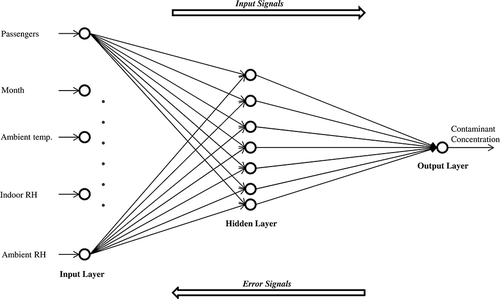
The number of neurons in the input, hidden, and output layers for any network depends on the problem considered. Accordingly, the number of neurons in the input layer and the output layer will be equivalent to the number of variables considered in the corresponding layer. If there are fewer neurons in the hidden layer, then the required accuracy may not be reached. Considering more neurons in the hidden layer may cause “overfitting” or “overtraining” that reduces the generalization capacity of the network. Thus, the selection of optimal number of neurons in the hidden layer is based on the mean absolute error (MAE) and the root mean square error (RMSE) statistics obtained from running the BPN with the associated data sets. Table 2 presents the MAE and RMSE statistics obtained from running the BPN for CO₂ with RT data set. From Table 2, one can observe that the BPN-CO₂-RT with seven neurons in the single hidden layer produced the best results. The MAE and the RMSE in Table 2 were within 8% of the maximum CO₂ reading. Similar trends were observed on considering the other monitored in-bus contaminants. BPN models developed with RT, PD_G, and TD data sets were referred as the BPN-RT, BPN-PD_G, and BPN-TD, respectively.

Table 2. Prediction results to determine the optimal number of neurons in the single hidden layer of BPN-CO₂-RT

	Number of hidden neurons
Statistical parameters	3	4	5	6	7	8	9	10	12	16
MAE (ppm)	100.42	83.60	77.49	75.63	70.26	83.31	85.07	126.28	79.01	72.36
RMSE (ppm)	121.15	106.86	101.29	98.77	93.65	106.28	108.06	151.29	102.65	98.57

Radial basis function network

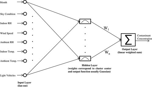
Radial basis functions (RBFs) were first introduced by Powell (1977) to solve the real multivariate interpolation problem. In the field of ANNs, radial basis functions were first used by Broomhead and Lowe (1988) in developing feed-forward networks. An RBF network (RBFN) is also a “supervised” learning method having three layers: an input layer, a hidden layer with nonlinear radial basis activation function, and a linear output layer. Figure 2 illustrates the structure of the RBFN for CO using the RT data set with the input, hidden, and output layers indicated from left to right. The independent variables affecting in-bus air quality are fed into the input layer that simply acts as a fan-out layer to feed the values to each of the neurons in the hidden layer and does not perform any processing. The hidden layer performs a nonlinear mapping from input space into a usually higher dimensional space in which patterns get linearly separable—that is, the transformation from the input layer to the hidden layer is nonlinear (Haykin, 1994). The hidden layer has a variable number of neurons with each neuron having a radial basis function (generally Gaussian function) centered on a point with as many dimensions as there are predictor variables. The spread (radius) of the radial basis function may vary for each dimension. At the input of each neuron in the hidden layer, the distance between neuron center and the input vector (Euclidean distance) is computed. The output of the neuron in the hidden layer is then computed by applying the basis function to this distance. The output layer (with the predicted in-bus contaminants) performs a simple weighted sum of the linear neuron output from the hidden layer and unity bias; that is, the transformation from the hidden layer to the output layer is linear (Haykin, 1994). In an RBFN, the neurons in the hidden layer are added up until the desired accuracy (0.001) is reached for a given spread. RBFN models developed with RT, PD_G, and TD data sets were referred as the RBFN-RT, RBFN-PD_G, and RBFN-TD, respectively.

Figure 2. Architecture of the RBFN-CO-RT.

Hybrid genetic-algorithm-based neural network

Genetic algorithms (GAs) are the optimization algorithms based on the mechanics of genetics, that is, the idea of the survival of the fittest (Karr et al., 1995). GAs generate a competitive set of solutions and then the solution evolves through the process of natural selection, where poor solutions die out and better solutions survive to reproduce. This process is repeated until the optimal solution is reached by the GA. The concept of GA was first introduced by Holland (1975) and further developed by Goldberg (1989) and Michalewicz (1996). GAs provide robust and reliable solutions for highly complex, nonlinear search and optimization problems, which previously could not be solved (Holland, 1995; Schwefel, 1995). The use of GAs has been increasing rapidly and they are mainly used in combination with other neural network models for extracting decision rules (Blackmore and Bossamaier, 2003) and for selecting the input parameters and defining the model structure for predicting atmospheric contaminants (Niska et al., 2004).

The use of GAs together with BPNs was initially explored by Dong et al. (2010) and Kadiyala et al. (2011). The current study extended the work by Kadiyala et al. (2011) to develop hybrid GA based neural networks using the BP mechanism. A hybrid GA-based neural network is fundamentally a BPN, with the only exception being that the weight matrix was attained from performing the genetic operations under optimal convergence conditions. Different options (population, fitness scaling, selection, reproduction, mutation, crossover, migration, algorithm settings, hybrid functions, and stopping criteria) need to be specified before running a GA. A comprehensive step-by-step procedure to determining the optimal GA parameters (based on the “fitness”) and extraction of the ideal weight matrix under optimal GA conditions were discussed in detail elsewhere (Kadiyala et al., 2011).

The methodology associated with the development of hybrid GA based neural network models can be divided into two phases: training/validation and testing. In the training/validation phase, a seven (ideal number) neuron single hidden layer BPN with random initial weights was coded in MATLAB to run with the GA option, that is, “Optimization Tool–ga solver.” The best chromosome, that is, the ideal weight matrix, which represented the optimal or near-optimal solution to the in-bus air quality prediction problem, was obtained when the GA converged under optimal conditions as tabulated in Table 3. The testing phase involved coding of the seven-neuron single hidden layer BPN with incorporation of the ideal weight matrix extracted from optimal GA conditions (in the training/validation phase) to predict the monitored in-bus contaminants. Hybrid GA-based neural network models developed with RT, PD_G, and TD data sets were referred as the GART, GAPD_G, and GATD, respectively.

Table 3. Summary of the optimal conditions used for running GA

Options		Optimal conditions
Population	Creation function	Uniform
	Population size	20
Fitness scaling		Rank
Selection		Roulette
Reproduction	Elite count	2
	Crossover fraction	0.8
Mutation		Uniform
Crossover		Scattered
Migration	Direction	Forward
	Fraction	0.2
	Interval	20
Algorithm settings	Initial penalty	10
	Penalty factor	100
Hybrid function		None
Stopping criteria	Generations	4000
	Time limit	Inf
	Fitness limit	0.001
	Stall generations	50
	Stall time limit	Inf
	Function tolerance	1e-6
	Nonlinear constraint tolerance	1e-6

Model validation

A good air quality model developed needs to provide adequate and reasonable estimates of the monitored observations. It is necessary to use statistical metrics to validate the developed air quality models. Air quality modelers have traditionally adopted the use of “holdout” validation methodology and determined the performance of model predictions using a set of operational performance measures. The holdout validation methodology was performed by further dividing the data sets (RT, PD_G, TD) into three subsets, namely, the training set (60%), the validation set (20%), and the test set (20%). The training set was used for learning and the validation set was used for adjusting the neural network parameters. The test set (that sufficiently represented the corresponding complete data set comprised of 20% of the data points extracted from each month during the monitoring period between April 2007 and March 2008), independent of the training and validation sets, was used to assess the performance of ANN-based IAQ models using a set of operational performance measures as discussed in the following.

Based on a comprehensive review of the literature on air quality model evaluation, Kadiyala and Kumar (2012d) enumerated a complete list of performance metric criteria to validate indoor and atmospheric air quality models with emphasis on the modeling attributes of the extreme-end (i.e., peak-end/low-end) concentrations and the mid-range concentrations. The statistical performance measures, namely, correlation (CORR), slope of the regression line (m), ratio of the intercept of regression line to the average observed concentrations (b/C₀), normalized mean square error (NMSE), fractional bias (FB), fractional variance (FV), fraction of predictions within a factor of two of the observations (FA2), model comparison measure (MCM₂), geometric mean bias (MG), geometric mean variance (VG), revised index of agreement (IOA_r), scatter plots, quantile–quantile (Q-Q) plots, and bootstrap 95% confidence interval estimates over NMSE, FB, CORR, VG, and MG were recommended to be used for mid-range IAQ model validation. The study also recommended a set of primary performance measures (Spearman rank correlation coefficient [ρ], m, b/C₀, FV, FA2, robust highest concentration ratio [RHC_ratio], MCM₂, MG, VG, scatter plots, Q-Q plots, bootstrap 95% confidence interval estimates over MG and VG) and a set of secondary performance measures (IOA_r, accuracy of paired peaks [A_p]) for IAQ model validation, when the emphasis was on the peak-end concentrations. With the exception of RHC_ratio and A_p, all other performance measures recommended for the peak-end IAQ model validation were recommended to be used for the low-end IAQ model validation. Refer to Kadiyala and Kumar (2012d) for additional details on the criteria used for selection and ranking of the operational model performance measures, based on the attributes of extreme-end and mid-range IAQ modeling.

An IAQ model is considered to be ideal and perfect when b/C₀, NMSE, FB, FV, and MCM₂ statistics are equal to zero; CORR, ρ, m, FA2, RHC_ratio, MG, VG, IOA_r, and A_p statistics are equal to one; and the scatter plots and the Q-Q graphical representations have the points plotted along the identity line (i.e., 1:1 line or a 45˚ line). However, models are rarely perfect in real life. Based on the recommendations made by Kadiyala and Kumar (2012d), an IAQ model is deemed acceptable from both extreme-end and mid-range modeling perspectives if it meets the criteria of (i) 0.9 ≤ CORR ≤ 1.0, (ii) 0.75 ≤ m ≤ 1.25, (iii) –25 ≤ b/C₀ (%) ≤ 25, (iv) 0 ≤ NMSE ≤ 0.25, (v) –0.25 ≤ FB ≤ 0.25, (vi) –0.5 ≤ FV ≤ 0.5, (vii) 0.8 ≤ FA2 ≤ 1.2, (viii) 0 ≤ MCM₂ ≤ 1.2, (ix) 0.8 ≤ MG ≤ 1.2, (x) 0.8 ≤ VG ≤ 1.2, (xi) 0.8 ≤ IOA_r ≤ 1.0, (xii) 0.9 ≤ ρ ≤ 1.0, (xiii) 0.8 ≤ RHC_ratio ≤ 1.2, and (xiv) –15 ≤ A_p ≤ 15. In addition to the already-mentioned criteria, the degree of closeness of plotted points in the scatter and Q-Q graphical representations to the identity line can help determine the superiority of one model over the other. In this study, the performance measures of m, b/C₀, FV, ρ, RHC_ratio, MCM₂, IOA_r, and A_p were computed using Microsoft Excel, while CORR, NMSE, FB, FA2, MG, VG, and bootstrap 95% confidence interval estimates over NMSE, r, FB, MG, and VG were computed using the BOOT v2.0. Graphical representations of the scatter plots and the Q-Q plots were obtained from using the MINITAB 16 and MathWorks MATLAB 2011b software, respectively.

On the contrary to general air quality model evaluation procedure, ANN modelers have preferred the use of “cross-validation” methodology and determined the performance of model predictions using the averaged cross-validation errors. In addition to validating the developed ANN-based IAQ models with the “holdout” predictions using a set of operational performance measures recommended by Kadiyala and Kumar (2012d), this study computed the threefold cross-validated root mean square error. To perform the threefold cross validation (3-fold CV), the data sets (RT, PD_G, TD) were randomly divided into three independent equivalent subsets. ANN-based IAQ models were trained and validated using two subsets and the predictive error (RMSE) over the third subset (test set) was determined. The process is repeated thrice such that each of the three subsets is used as a test set for once and the RMSEs from the three runs were averaged. The holdout RMSE and the averaged 3-fold CV RMSE were divided with the mean observed values and multiplied by 100 to obtain a nondimensional prediction error term referred as RMSE (%).

Results and Discussion

Table 4 presents the statistical performance measures computed for the BP-, RBF-, and GA-based neural network models with RT, PD_G, and TD data sets for the monitored in-bus contaminant of CO₂ obtained from the holdout validation. From Table 4, one can note that the BPN models did not meet the stringent IAQ model acceptance criteria of 0.9 ≤ CORR ≤ 1.0, 0.75 ≤ m ≤ 1.25, −25 ≤ b/C₀ (%) ≤ 25, −0.5 ≤ FV ≤ 0.5, 0.8 ≤ IOA_r ≤ 1.0, and 0.9 ≤ ρ ≤ 1.0, while the RBFN models did not meet the criteria for CORR, IOA_r, and ρ. Only the GA-based neural network models (GATD, GAPD_G, GART) satisfied all the 14 IAQ model acceptance criteria considered in this study. There was not much difference between the computed performance measures of GATD and GART models for the in-bus CO₂ contaminant concentration.

Table 4. CO₂ statistical performance measures

	MEAN	SIGMA	CORR	m	b/C0(%)	NMSE	FB	FV	FA2	MCM2	IOAr	ρ	RHCratio	Ap	MG	VG
MODEL	Arithmetic values														Log values
OBS.	577.950	141.770	1.000	1.000	0.000	0.000	0.000	0.000	1.000	0.000	1.000	1.000	1.000	0.000	1.000	1.000
BPN-TD	579.850	104.290	0.722	0.531	47.233	0.030	–0.003	0.595	0.996	0.360	0.677	0.741	0.854	–21.058	0.980	1.030
BPN-PDG	581.550	95.800	0.662	0.447	55.921	0.030	–0.006	0.746	0.996	0.367	0.639	0.684	0.804	–24.883	0.980	1.030
BPN-RT	597.890	83.960	0.633	0.375	65.969	0.040	–0.034	0.961	1.000	0.360	0.619	0.624	0.894	–10.438	0.950	1.040
RBFN-TD	580.660	128.190	0.850	0.769	23.599	0.020	–0.005	0.201	1.000	0.249	0.748	0.861	1.002	–0.245	0.990	1.020
RBFN-PDG	575.830	127.730	0.869	0.783	21.334	0.010	0.004	0.208	1.000	0.268	0.778	0.884	0.933	0.993	1.000	1.010
RBFN-RT	576.230	128.890	0.854	0.777	22.040	0.020	0.003	0.190	1.000	0.270	0.769	0.863	0.948	0.160	1.000	1.020
GATD	560.130	142.130	1.000	1.002	–3.308	0.000	0.031	–0.005	1.000	0.032	0.923	1.000	0.981	–1.388	1.030	1.000
GAPDG	559.800	141.010	0.985	0.980	–1.142	0.000	0.032	0.011	1.000	0.099	0.912	0.981	0.970	–5.253	1.030	1.000
GART	535.080	140.280	0.994	0.984	–5.794	0.010	0.077	0.021	1.000	0.092	0.812	0.992	0.935	–7.973	1.080	1.010

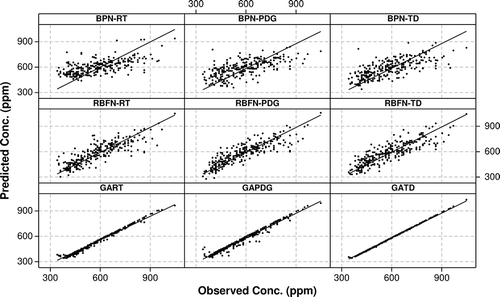
Table 5 presents the bootstrap 95% confidence limits computed for the BP-, RBF-, and GA-based neural network models with the RT, PD_G, and TD data sets for CO₂ obtained from the holdout validation. From Table 5, one can notice that irrespective of the data set considered, all three neural network techniques (BP-, RBF-, GA-based neural networks) were significantly different from zero for NMSE, CORR, MG, and VG statistics. The BPN-RT and the three GA-based neural network models exhibited the significant difference to zero property with FB, which was not the case with the remaining BPN and RBFN models. Figure 3 presents the scatter plots obtained for the in-bus CO₂ contaminant using the BP-, RBF-, and GA-based neural networks with RT, PD_G, and TD data sets. In summary of the discussion on the performance of the developed in-bus CO₂ concentration models using the holdout validation, one can conclude that the GA-based neural networks outperformed the BPN and the RBFN models, and the GART model accounted for majority of the variance observed in the in-bus CO₂ contaminant concentrations.

Table 5. CO₂ bootstrap 95% confidence limits

Model(s)	NMSE	FB	CORR	VG	MG
BPN-TD	0.023–0.035	−0.022–0.017	0.657–0.786	1.000–1.000	0.966–1.004
BPN-PDG	0.027–0.040	−0.026–0.016	0.594–0.730	1.000–1.000	0.959–1.001
BPN-RT	0.030–0.042	−0.055–−0.011	0.550–0.715	1.000–1.000	0.928–0.969
RBFN-TD	0.014–0.020	−0.020–0.010	0.819–0.881	1.000–1.000	0.976–1.006
RBFN-PDG	0.012–0.018	−0.010–0.018	0.838–0.900	1.000–1.000	0.986–1.014
RBFN-RT	0.013–0.020	−0.012–0.018	0.818–0.890	1.000–1.000	0.985–1.014
GATD	0.001–0.001	0.030–0.033	0.999–1.000	1.000–1.000	1.032–1.035
GAPDG	0.002–0.004	0.027–0.037	0.979–0.992	1.000–1.000	1.028–1.040
GART	0.006–0.007	0.073–0.081	0.991–0.997	1.000–1.000	1.080–1.089
Note: The robust 95% confidence limits are based on the usual Student's t approach using calculated mean and standard deviation.

Figure 3. Scatter plots for CO₂ observed and predicted values.

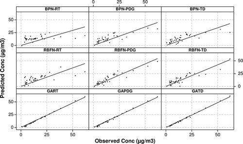
Table 6 presents the statistical performance measures computed for the GA-based neural network models with RT, PD_G, and TD data sets for the monitored in-bus contaminants of CO, NO, SO₂, 0.3–0.4 particle numbers, 0.4–0.5 particle numbers, PM_1.0, and PM_2.5 obtained from the holdout validation. The three GA-based neural network models developed for the in-bus contaminant concentrations of CO, SO₂, 0.3–0.4 particle numbers, PM_1.0, and PM_2.5 met all the IAQ model acceptance criteria. Of the three GA-based neural network models developed for NO concentrations inside the bus, only the GART models satisfied all the IAQ model acceptance criteria; GATD and GAPD_G models did not meet the stringent guidelines for ρ. The GART models developed for in-bus 0.4–0.5 particle numbers entirely satisfied the IAQ performance measures criteria, while the GATD and GAPD_G models failed to meet the stringent guidelines of MG and VG. Figures 4 to 10 illustrate the scatter plots obtained for the in-bus contaminants of CO, NO, SO₂, 0.3–0.4 particle numbers, 0.4–0.5 particle numbers, PM_1.0, and PM_2.5, respectively, using the BP-, RBF-, and GA-based neural networks with RT, PD_G, and TD data sets. In view of the discussion on comparing the performance of the three GA-based neural network models with holdout validation, one can conclude that only the GART models satisfied all the stringent IAQ model acceptance criteria and the GART modeling approach proved to be an effective/optimal method of modeling in-bus air quality, considering the development of valid IAQ models with elimination of the insignificant independent input variables that cause noise.

Table 6. Statistical performance measures for GA-based neural networks for CO, NO, SO₂, 0.3–0.4 particle numbers, 0.4–0.5 particle numbers, PM_1.0, and PM_2.5

	MEAN	SIGMA	CORR	m	b/C0(%)	NMSE	FB	FV	FA2	MCM2	IOAr	ρ	RHCratio	Ap	MG	VG
	Arithmetic values														Log values
CO
OBS.	14.360	9.500	1.000	1.000	0.000	0.000	0.000	0.000	1.000	0.000	1.000	1.000	1.000	0.000	1.000	1.000
GATD	13.540	9.490	1.000	0.998	–5.470	0.000	0.058	0.003	0.975	0.054	0.944	0.999	0.974	–1.568	1.130	1.040
GAPDG	13.490	9.490	0.994	0.993	–5.366	0.010	0.063	0.002	0.936	0.116	0.940	0.991	0.966	–2.032	1.150	1.090
GART	12.130	9.060	0.955	0.910	–6.496	0.070	0.168	0.096	0.829	0.261	0.817	0.934	0.987	–0.696	1.180	1.150
NO
OBS.	0.460	0.370	1.000	1.000	0.000	0.000	0.000	0.000	1.000	0.000	1.000	1.000	1.000	0.000	1.000	1.000
GATD	0.420	0.350	0.993	0.952	–4.559	0.020	0.097	0.084	1.000	0.345	0.865	0.858	0.957	–2.162	1.110	1.040
GAPDG	0.430	0.340	0.967	0.916	2.121	0.050	0.064	0.108	0.964	0.716	0.851	0.772	0.965	–2.193	1.060	1.070
GART	0.440	0.350	0.994	0.953	0.738	0.010	0.040	0.085	1.000	0.084	0.951	0.976	0.923	–7.580	1.040	1.010
SO2
OBS.	0.260	0.060	1.000	1.000	0.000	0.000	0.000	0.000	1.000	0.000	1.000	1.000	1.000	0.000	1.000	1.000
GATD	0.240	0.060	0.991	0.924	2.115	0.000	0.057	0.145	1.000	0.136	0.835	0.996	0.968	–5.009	1.050	1.010
GAPDG	0.240	0.060	0.933	0.907	2.989	0.010	0.066	0.060	1.000	0.374	0.812	0.936	1.003	–1.743	1.070	1.020
GART	0.250	0.060	0.996	0.977	1.484	0.000	0.009	0.040	1.000	0.044	0.972	0.994	0.984	–5.064	1.010	1.000
0.3–0.4 µm sized particle numbers
OBS.	132231.530	140764.280	1.000	1.000	0.000	0.000	0.000	0.000	1.000	0.000	1.000	1.000	1.000	0.000	1.000	1.000
GATD	130146.100	140657.330	0.997	0.996	–1.208	0.010	0.016	0.001	0.973	0.476	0.975	0.971	1.003	–0.176	1.030	1.070
GAPDG	127412.430	140692.470	1.000	0.999	–3.592	0.000	0.037	0.001	1.000	0.241	0.974	0.999	0.994	–0.674	1.080	1.010
GART	119305.800	140386.140	1.000	0.997	–9.490	0.010	0.103	0.003	0.959	0.603	0.931	0.998	0.979	–1.810	1.971	1.090
0.4–0.5 µm sized particle numbers
OBS.	36177.180	37649.270	1.000	1.000	0.000	0.000	0.000	0.000	1.000	0.000	1.000	1.000	1.000	0.000	1.000	1.000
GATD	31375.080	37714.590	0.998	0.999	–13.244	0.030	0.142	–0.002	0.836	0.912	0.907	0.974	0.954	–1.392	1.350	1.220
GAPDG	32817.510	38317.200	0.997	1.015	–10.820	0.020	0.097	–0.018	0.877	0.920	0.935	0.968	0.991	–1.826	1.310	1.220
GART	35055.510	37979.450	1.000	1.009	–3.962	0.000	0.031	–0.009	1.000	0.307	0.979	0.998	1.008	–0.604	1.080	1.010
PM1.0
OBS.	12.200	11.340	1.000	1.000	0.000	0.000	0.000	0.000	1.000	0.000	1.000	1.000	1.000	0.000	1.000	1.000
GATD	11.550	11.330	0.998	0.997	–5.030	0.010	0.055	0.001	1.000	0.281	0.958	0.992	0.971	–0.971	1.090	1.020
GAPDG	11.280	11.250	0.997	0.988	–6.430	0.010	0.079	0.009	0.947	0.580	0.940	0.982	0.950	–3.306	1.160	1.080
GART	11.520	11.310	0.999	0.996	–5.191	0.010	0.058	0.003	0.921	0.592	0.954	0.995	0.988	–2.600	1.140	1.060
PM2.5
OBS.	14.950	12.990	1.000	1.000	0.000	0.000	0.000	0.000	1.000	0.000	1.000	1.000	1.000	0.000	1.000	1.000
GATD	14.230	12.950	0.999	0.996	–4.394	0.000	0.049	0.003	1.000	0.265	0.960	0.994	0.975	–0.877	1.080	1.010
GAPDG	13.920	12.870	0.997	0.988	–5.693	0.010	0.071	0.009	0.947	0.561	0.943	0.984	0.950	–3.074	1.150	1.070
GART	13.890	12.900	0.998	0.992	–6.273	0.010	0.073	0.007	0.921	0.590	0.940	0.994	1.003	–2.852	1.160	1.060

Figure 4. Scatter plots for CO observed and predicted values.

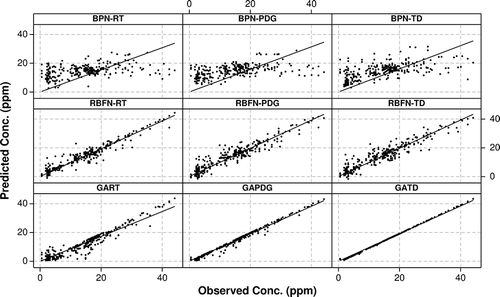
Figure 5. Scatter plots for NO observed and predicted values.

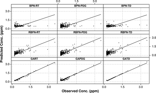
Figure 6. Scatter plots for SO₂ observed and predicted values.

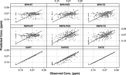
Figure 7. Scatter plots for 0.3–0.4 µm sized particle numbers observed and predicted values.

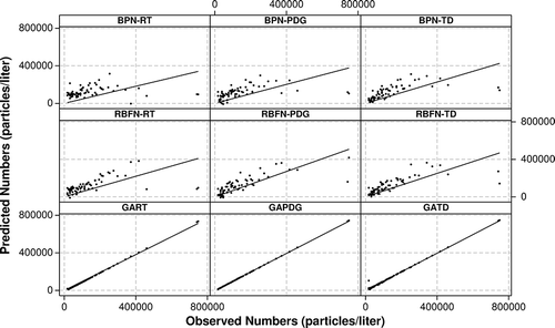
Figure 8. Scatter plots for 0.4–0.5 µm sized particle numbers observed and predicted values.

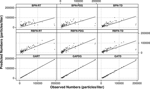
Figure 9. Scatter plots for PM_1.0 observed and predicted values.

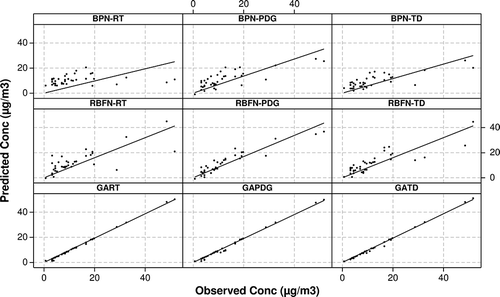
Figure 10. Scatter plots for PM_2.5 observed and predicted values.

Irrespective of the in-bus contaminant considered, none of the BPN and RBFN models met all the stringent IAQ guideline criteria; the only exception was the RBFN-RT model developed for CO concentration, as can be observed from the supplemental document Tables S1 through S7 (Kadiyala et al., 2013). The bootstrap 95% confidence limits for the in-bus contaminants of CO, NO, SO₂, 0.3–0.4 particle numbers, 0.4–0.5 particle numbers, PM_1.0, and PM_2.5, for the BP-, RBF-, and GA-based neural network models with RT, PD_G, and TD datasets were summarized in the supplemental document Tables S8 through S14 (Kadiyala et al., 2013). Q-Q plots for the in-bus contaminants of CO₂, CO, NO, SO₂, 0.3–0.4 particle numbers, 0.4–0.5 particle numbers, PM_1.0, and PM_2.5, obtained from the development of BP-, RBF-, and GA-based neural networks with RT, PD_G, and TD data sets were also documented as Figures S1 through S8 in the supplemental document (Kadiyala et al., 2013). In summary of the discussion on comparing the performance of BPN and RBFN models with holdout validation, none of the developed in-bus air quality models were valid; the only exception was the RBFN-RT model developed for CO concentrations.

Table 7 presents a summary of the holdout validation and the 3-fold CV prediction errors, that is, RMSE (%), for the developed in-bus air quality models. The prediction errors with the holdout validation and the 3-fold CV varied in the ranges 0.98–17.57% and 0.91–10.16% for the BPN models, 0.74–13.13% and 0.62–6.36% for the RBFN models, and 0.13–2.09% and 0.08–3.94% for the GA-based neural network models, respectively. On considering the GART models, one can note that the 3-fold CV RMSE (%) was relatively less than the corresponding holdout validation RMSE (%), with the exception of CO and PM_1.0 in-bus contaminants.

Table 7. Summary of the holdout validation and the 3-fold CV prediction errors for the developed in-bus air quality models

		Prediction error for in-bus air quality models: RMSE (%)
Contaminant	Validation method	BPN-TD	BPN-PDG	BPN-RT	RBFN-TD	RBFN-PDG	RBFN-RT	GATD	GAPDG	GART
CO2	Holdout	0.98	1.06	1.11	0.75	1.06	0.74	0.18	1.06	0.45
	3-fold CV	0.91	0.92	1.04	0.62	0.66	1.07	0.47	0.62	0.31
CO	Holdout	3.23	3.45	3.59	1.41	1.34	1.13	0.35	0.56	1.55
	3-fold CV	2.53	3.45	2.74	1.20	1.83	1.83	0.84	1.20	3.94
NO	Holdout	4.21	4.23	4.34	3.00	2.77	3.02	0.74	1.15	0.53
	3-fold CV	3.68	4.02	4.14	2.61	2.62	4.01	2.38	2.22	0.26
SO2	Holdout	1.41	1.51	1.54	1.14	1.22	1.50	0.39	0.66	0.13
	3-fold CV	1.52	1.61	1.57	1.11	1.10	1.52	1.28	1.30	0.08
0.3–0.4 µm sized particle numbers	Holdout CV3-fold CV	12.02 6.16	13.45 7.09	15.12 7.34	10.69 5.03	9.78 5.06	13.13 5.96	1.17 0.61	0.52 0.35	1.40 0.99
0.4–0.5 µm sized particle numbers	Holdout3-fold CV	11.68 5.71	12.47 6.50	13.31 6.70	10.98 4.71	7.89 4.72	9.38 4.64	2.09 1.99	1.68 2.38	0.54 0.17
PM1.0	Holdout	13.11	11.68	17.57	9.40	6.93	11.49	1.42	1.99	1.33
	3-fold CV	9.31	8.55	10.16	6.36	6.17	5.98	1.52	1.61	2.18
PM2.5	Holdout	10.58	9.77	14.14	7.25	6.29	11.10	1.18	1.78	1.55
	3-fold CV	8.51	7.92	9.18	5.48	5.48	5.33	1.41	1.48	1.26

The development of valid in-bus air quality prediction models is useful for managing air quality and for the development of practical exposure models by computing the time-weighted average (TWA) concentration. The results from the exposure models could then be used to compare against the current IAQ guidelines as discussed by Kadiyala et al. (2010) and health standards. As an example, if the TWA in-bus contaminant concentrations or the peak concentrations exceed the recommended guidelines for a bus, the public transit authorities could increase the air changes per hour, which can prevent the accumulation of in-bus contaminants beyond the permissible limits.

Conclusion

A novel methodology to accurately predict the in-bus contaminant concentrations was developed and successfully applied to an experimental field program. The statistically significant variables affecting each monitored contaminant were determined from performing the ANOVA as a complimentary sensitivity analysis to the regression tree results. The identified statistically significant variables from aforementioned step were then used as input parameters to develop GA-based neural network models, referred as the GART models, which made valid predictions of the in-bus contaminant levels. Performance of the three ANNs—BP-, RBF-, and GA-based neural networks—were evaluated with the model performance measures using three data sets, namely, RT, PD_G, and TD. Irrespective of the data set considered, GA-based neural network models performed much better than the BPN and RBFN models. The GART modeling approach captured majority of the variation observed in the in-bus contaminants and it is hoped that the use of GART models will be examined extensively in other fields of study also. It should be noted that this study is based on the data collected inside a single transit bus and that, while it illustrates a new methodology to modeling in-bus air quality, the results may not be generalizable.

Acknowledgment

The authors thank the U.S. Department of Transportation and Toledo Area Regional Transit Authority (TARTA) for the alternate fuel grant awarded to the Intermodal Transportation Institute of the University of Toledo. The authors also express their sincere gratitude to the TARTA management and the employees for their interest and involvement in this work during data collection throughout the grant period. The authors do not have any financial relationships/gains in relation to using the Grimm 1.108 instrument, Yes Plus instrument, and commercial software package used in this study such as MATLAB. The views expressed in this paper are those of the authors alone and do not represent the views of the funding organizations.

References

- Blackmore , K. and Bossomaier , T. 2003 . Using a Neural Network and Genetic Algorithm to Extract Decision Rules . Proceedings of the 8th Australian and New Zealand Conference on Intelligent Information Systems , 12 December 10 : 187 – 191 . Sydney, Australia
- Broomhead , D.S. and Lowe , D. 1988 . Multivariable Functional Interpolation and Adaptive Networks . Complex Syst. , 2 : 321 – 355 . doi: 10.1234/12345678
- Brunelli , U. , Piazza , V. , Pignato , L. , Sorbello , F. and Vitabile , S. 2007 . Two-Days Ahead Prediction of Daily Maximum Concentrations of SO2, O3, PM10, NO2, CO in the Urban Area of Palermo, Italy . Atmos. Environ. , 41 : 2967 – 2995 . doi: 10.1016/j.atmosenv.2006.12.013
- Bryson , A.E. and Ho , Y.C. 1969 . Applied Optimal Control: Optimization, Estimation and Control , New York , NY : Blaisdell Publications .
- Dong , X. , Wang , S. , Sun , R. and Zhao , S. Design of Artificial Neural Networks Using a Genetic Algorithm to Predict Saturates of Vacuum Gas Oil . Petrol. Sci. , 7 118 – 122 . doi: 10.1007/s12182-010-0015-y
- Esber , L.A. and El-Fadel , M. 2008 . In-Vehicle CO Ingression: Validation Through Field Measurements and Mass Balance Simulations . Sci. Total Environ. , 394 : 75 – 89 . doi: 10.1016/j.scitotenv.2008.01.034
- Gardner , M.W. and Dorling , S.R. 1998 . Artificial Neural Networks (the Multilayer Perceptron)—A Review of Applications in the Atmospheric Sciences . Atmos. Environ. , 32 : 2627 – 2636 . doi: 10.1016/S1352-2310(97)00447-0
- Gardner , M.W. and Dorling , S.R. 1999 . Neural Network Modelling and Prediction of Hourly NOx and NO2 Concentrations in Urban Air in London . Atmos. Environ. , 33 : 709 – 719 . doi: 10.1016/S1352-2310(98)00230-1
- Goldberg , D.E. 1989 . Genetic Algorithms in Search, Optimization and Machine Learning , Boston , MA : Addison-Wesley Longman .
- Haykin , S. 1994 . Neural Networks: A Comprehensive Foundation , 2nd , New York , NY : Macmillan Publications .
- Holland , J.H. 1975 . Adaptation in Natural and Artificial Systems , Arbor : Ann University of Michigan Press .
- Holland , J.H. 1995 . Hidden Order: How Adaptation Builds Complexity , Reading , MA : Addison-Wesley .
- Hornik , K. , Stinchcoombe , M. and White , H. 1989 . Multi Layer Feed Forward Networks Are Universal Approximators . Neural Networks , 2 : 359 – 366 . doi: 10.1016/0893-6080(89)90020-8
- Kadiyala , A. 2012 . Development and Evaluation of an Integrated Approach to Study In-Bus Exposure Using Data Mining and Artificial Intelligence Methods. PhD dissertation , Toledo , OH : University of Toledo .
- Kadiyala , A. , Kaur , D. and Kumar , A. 2011 . Application of MATLAB to Select an Optimum Performing Genetic Algorithm for Predicting In-Vehicle Pollutant Concentrations . Environ. Prog. Sustainable Energy. , 29 : 398 – 405 . doi: 10.1002/ep.10527
- Kadiyala , A. , Kaur , D. and Kumar , A. 2013 . Development of Hybrid Genetic Algorithm Based Neural Networks Using Regression Trees for Modeling . Air Quality Inside a Public Transportation Bus (Supplementary Document). ,
- Kadiyala , A. and Kumar , A. 2008 . Application of CART and Minitab Software to Identify Variables Affecting Indoor Concentration Levels . Environ. Prog. , 27 : 160 – 168 . doi: 10.1002/ep.10292
- Kadiyala , A. and Kumar , A. 2011a . Quantification of In-Vehicle Gaseous Contaminants of Carbon Dioxide and Carbon Monoxide Under Varying Climatic Conditions . Air Qual. Atmos. Health. , doi: 10.1007/s11869-011-0163-2
- Kadiyala , A. and Kumar , A. 2011b . Study of In-Vehicle Pollutant Variation in Public Transport Buses Operating on Alternative Fuels in the City of Toledo, Ohio . Open Environ. Biol. Monit. J. , 4 : 1 – 20 . doi: 10.2174/1875040001104010001
- Kadiyala , A. and Kumar , A. 2012a . “ Examination of Two Different Mathematical Techniques for Determining the Important Factors Affecting Indoor Air Quality ” . In Handbook of Genetic Algorithms: New Research , Edited by: Muñoz , A.R. and Rodriguez , I.G. p. 93–112. New York: Nova Science Publishers .
- Kadiyala , A. and Kumar , A. 2012b . Development and Application of a Methodology to Identify and Rank the Important Factors Affecting In-Vehicle Particulate Matter . J.Hazard. Mater. , 213–214 : 140 – 146 . doi: 10.1016/j.jhazmat.2012.01.072
- Kadiyala , A. and Kumar , A. 2012c . An Examination of the Sensitivity of Sulfur Dioxide, Nitric Oxide, and Nitrogen Dioxide Concentrations to the Important Factors Affecting Air Quality Inside a Public Transportation Bus . Atmosphere , 3 : 266 – 287 . doi: 10.3390/atmos3020266
- Kadiyala , A. and Kumar , A. 2012d . Guidelines for Operational Evaluation of Air Quality Models , Saarbrücken : LAP LAMBERT Academic .
- Kadiyala , A. , Kumar , A. and Vijayan , A. 2010 . Study of Occupant Exposure of Drivers and Commuters With Temporal Variation of In-Vehicle Pollutant Concentrations in Public Transport Buses Operating on Alternative Diesel Fuels . Open Environ. Eng. J. , 3 : 55 – 70 . doi: 10.2174/1874829501003010055
- Karr , C.L. , Weck , B. , Massart , D.L. and Vankeerberghen , P. 1995 . Least Median Squares Curve Fitting Using Genetic Algorithm . Eng. Appl. Artif. Intell. , 8 : 177 – 189 . doi: 10.1016/0952-1976(94)00064-T
- Khare , M. and Nagendra , S.M.S. 2006 . Artificial Neural Networks in Vehicular Pollution Modeling , New York , NY : Springer-Verlag .
- Klepeis , N.E. , Nelson , W.C. , Ott , W.R. , Robinson , J.P. , Tsang , A.M. , Switzer , P. , Behar , J.V. , Hern , S.C. and Engelmann , W.H. 2001 . The National Human Activity Pattern Survey (NHAPS): A Resource for Assessing Exposure to Environmental Pollutants . J.Expos. Anal. Environ. Epidemiol. , 11 : 231 – 252 . doi: 10.1038/sj.jea.7500165
- Kolehmainen , M. , Martikainen , H. and Ruuskanen , J. 2001 . Neural Networks and Periodic Components Used in Air Quality Forecasting . Atmos. Environ. , 35 : 815 – 825 . doi: 10.1016/S1352-2310(00)00385-X
- Kukkonen , J. , Partanen , L. , Karppinen , A. , Ruuskanen , J. , Junninen , H. , Kolehmainen , M. and Gwynne , M. 2003 . Extensive Evaluation of Neural Network Models for the Prediction of NO2 and PM10 Concentrations, Compared With a Deterministic Modelling System and Measurements in Central Helsinki . Atmos. Environ. , 37 : 4539 – 4550 . doi: 10.1016/S1352-2310(03)00583-1
- Maier , H.R. and Dandy , G.C. 2001 . Neural Network Based Modeling of Environmental Variables: A Systematic Approach . Math. Comput. Model. , 33 : 669 – 682 . doi: 10.1016/S0895-7177(00)00271-5
- Michalewicz , Z. 1996 . Genetic Algorithms + Data Structures = Evolution Programs , 3rd , New York , NY : Springer-Verlag .
- Moustris , K.P. , Ziomass , I.C. and Paliatsos , A.G. 2010 . 3-Day-Ahead Forecasting of Regional Pollution Index for the Pollutants NO2, CO, SO2, and O3 Using Artificial Neural Networks in Athens, Greece . Water Air Soil Pollut. , 209 : 29 – 43 . doi: 10.1007/s11270-009-0179-5
- National Climatic Data Center. 2011. NCDC http://cdo.ncdc.noaa.gov/ulcd/ULCD (http://cdo.ncdc.noaa.gov/ulcd/ULCD)
- Negnevitsky , M. 2005 . Artificial Intelligence: A Guide to Intelligent Systems , 2nd , Harlow : Pearson Education Limited .
- Niska , H. , Hiltunen , T. , Karppinen , A. , Ruuskanen , J. and Kolehmainen , M. 2004 . Evolving the Neural Network Model for Forecasting Air Pollution Time Series . Eng. Appl. Artif. Intell. , 17 : 159 – 167 . doi: 10.1016/j.engappai.2004.02.002
- Papanastasiou , D.K. , Melas , D. and Kioutsioukis , I. 2007 . Development and Assessment of Neural Network and Multiple Regression Models in Order to Predict PM10 Levels in a Medium-Sized Mediterranean City . Water Air Soil Pollut. , 182 : 325 – 334 . doi: 10.1007/s11270-007-9341-0
- Perez , P. , Trier , A. and Reyes , J. 2000 . Prediction of PM2.5Concentrations Several Hours in Advance Using Neural Networks in Santiago, Chile . Atmos. Environ. , 34 : 1189 – 1196 . doi: 10.1016/S1352-2310(99)00316-7
- Powell , M.J.D. 1977 . Restart Procedures for the Conjugate Gradient Method . Math. Prog. , 12 : 241 – 254 . doi: 10.1007/BF01593790
- Schwefel , H.P. 1995 . Evolution and Optimum Seeking , New York , NY : John Wiley .
- TARTA Routes, 2011. Route #20 http://www.tarta.com/wp-content/uploads/routes/20.pdf (http://www.tarta.com/wp-content/uploads/routes/20.pdf)