Aerosol species concentrations and source apportionment of ammonia at Rocky Mountain National Park

Abstract

Changes in ecosystem function at Rocky Mountain National Park (RMNP) are occurring because of emissions of nitrogen and sulfate species along the Front Range of the Colorado Rocky Mountains, as well as sources farther east and west. The nitrogen compounds include both oxidized and reduced nitrogen. A year-long monitoring program of various oxidized and reduced nitrogen species was initiated to better understand their origins as well as the complex chemistry occurring during transport from source to receptor. Specifically, the goals of the study were to characterize the atmospheric concentrations of nitrogen species in gaseous, particulate, and aqueous phases (precipitation and clouds) along the east and west sides of the Continental Divide; identify the relative contributions to atmospheric nitrogen species in RMNP from within and outside of the state of Colorado; identify the relative contributions to atmospheric nitrogen species in RMNP from emission sources along the Colorado Front Range versus other areas within Colorado; and identify the relative contributions to atmospheric nitrogen species from mobile sources, agricultural activities, and large and small point sources within the state of Colorado. Measured ammonia concentrations are combined with modeled releases of conservative tracers from ammonia source regions around the United States to apportion ammonia to its respective sources, using receptor modeling tools.

Implications:

Increased deposition of nitrogen in RMNP has been demonstrated to contribute to a number of important ecosystem changes. The rate of deposition of nitrogen compounds in RMNP has crossed a crucial threshold called the “critical load.” This means that changes are occurring to park ecosystems and that these changes may soon reach a point where they are difficult or impossible to reverse. Several key issues need attention to develop an effective strategy for protecting park resources from adverse impacts of elevated nitrogen deposition. These include determining the importance of previously unquantified nitrogen inputs within the park and identification of important nitrogen sources and transport pathways.

Introduction

Atmospheric nitrogen and sulfur species can cause a number of deleterious effects, including visibility impairment and changes in ecosystem function and surface water chemistry from atmospheric deposition. Within Rocky Mountain National Park (RMNP), an area of particular interest, wet deposition of inorganic nitrogen (nitrate and ammonium) currently contributes approximately 3 kg/ha/yr to total nitrogen input (Baron et al., 2011). Dry deposition of nitric acid (HNO₃) and particulate nitrate and ammonium (NH₄ ⁺) increases total measured nitrogen deposition to approximately 4 kg/ha/yr. These current nitrogen deposition flux values appear to represent approximately a 20-fold increase above preindustrial values for the western United States (Galloway et al., 1982, 1995; Hedin et al., 1995).

Increased deposition of nitrogen in RMNP has been demonstrated to contribute to a number of important ecosystem changes (for a review see Blett and Morris, 2004). Among these are changes in the chemistry of old-growth Engelmann spruce forests (Rueth and Baron, 2002), shifts in population of lake diatoms (Baron et al., 2000), excess nitrogen leakage into lakes and streams at certain times of the year (Campbell et al., 2000), and alterations in biogeochemical cycling associated with increased microbial activity in high elevation soils and talus (Campbell et al., 2000, 2002; Rueth and Baron, 2002). Several of these effects have been noted mainly on the east side of the Continental Divide that runs through RMNP. Nitrogen deposition levels have also been determined to be higher on the eastern slope of the park (Burns, 2003). Nitrate wet deposition has increased by approximately 10–20%, and ammonium wet deposition has increased by about 50% (Lehmann et al., 2005).

The Rocky Mountain Atmospheric Nitrogen and Sulfur (RoMANS) study was initiated to better understand the origins and physical/chemical and optical characteristics of nitrogen species, as well as the complex chemistry occurring during transport from source to receptor. Assessing changes in ambient concentrations of aerosol species and wet deposition as a function of changing ammonia and nitrogen oxide concentrations is dependent on a number of chemical and physical mechanisms, as well as meteorological conditions and transport characteristics. For example, ammonia will increase particle mass by reacting with acidic sulfate aerosols, nitric acid, and organic acids. With respect to the reaction of ammonia with nitric acid, the equilibrium between these species and the reaction product, ammonium nitrate, is temperature dependent and can go from predominantly gases to particles with the diurnal shifts in temperature. The condensation of ammonia onto particles is also dependent on the acidity of the particles and ambient relative humidity. These reactions do not necessarily take place at or near the source of ammonia, but over the transport pathways from source to receptor (Seinfeld and Pandis, 1998). Actually, sources of nitric acid, acidic sulfates, and organic acids are not likely to be associated with ammonia sources.

Increases in ammonia emissions will tend to increase and change the composition of particulate matter (PM) mass concentrations. Regardless of the chemical form and phase of the nitrogen, it will ultimately be deposited onto terrestrial or aquatic surfaces, but where these species are deposited does depend on the chemical form and phase of the nitrogen. For example, gaseous ammonia has higher deposition rates and will deposit closer to the sources, while ammoniated particulates can be transported hundreds of kilometers before deposition.

As part of the study, a monitoring program was initiated for one year, starting in November 2008. The monitoring program consisted of intensive, high time resolution measurements of particles, gas, wet deposition, and meteorology at a core site, subsequently referred to as the receptor site, near RMNP. This paper includes a discussion of aerosol species concentrations collected at RMNP, and because little effort has been focused on understanding sources responsible for elevated ambient ammonia concentrations in RMNP, an apportionment of measured ammonia concentrations to sources of ammonia using hybrid receptor modeling techniques is presented.

Measurements

A 12-month intensive monitoring program was conducted, starting on November 11, 2008. A summary of the measurements is included in Table 1. Gas-phase measurements were made continuously and in real time, with 1-min averaged data. Instrumentation was housed in a temperature-controlled (25 ± 5°C) shelter (National Park Service air quality shelter), collocated with the existing Interagency Monitoring of Protected Visual Environments (IMPROVE) (Hand et al., 2011) and Clean Air Status and Trends Network (CASTNET) (CASTNET, 2010) sites near the eastern boundary of RMNP.

Table 1 . Measurements at the core sites

Measurement	Instrument	Time resolution	Notes
PM2.5 inorganic ions and gases	Annular denuder/filter-pack sampler	24 hr	Cl^−, NO2 ^−, NO3 ^−, SO4 ^2−, Na^+, K^+, NH4 ^+, Mg^2+, Ca^2+, HNO3, NH3
PM2.5 inorganic ions	Particle-into-liquid sampler (PILS)–IC	15 min	Cl^−, NO2 ^−, NO3 ^−, SO4 ^2−, Na^+, K^+, NH4 ^+, Mg^2+, Ca^2+
PM2.5 mass, ions, elements, H, and OC/EC	IMPROVE sampler	24 hr	Components per IMPROVE protocol
PM10 mass	IMPROVE sampler	24 hr	Components per IMPROVE protocol
NOx, NOy, HNO3, TNx, NHx,gas, CO	Various continuous gas monitors	1 min	An estimate of reduced nitrogen other than ammonia.
Meteorological parameters	Met station	2 min	T, RH, WD, WS, Precip, SR,BP
Particle size distributions	Differential mobility particle sizing (DMPS) system, optical particle counter (OPC), aerodynamic particle sizer (APS)	15 min	0.05–10 µm diameter
Particle light scattering	Nephelometer	2 min	Ambient PM2.5 aerosol

The configuration of the gas-phase instrument is shown in Figure 1. Measurements of nitric oxide (NO) and NO_y were made using a Teledyne-API, Inc. (M200EU), NO_y chemiluminescence instrument (Fontijn et al., 1970; Fehsenfeld et al., 1987; Williams et al., 1998; Demerjian, 2000; Parrish and Fehsenfeld, 2000), with a detection limit of 50 ppt. For these studies, the converter temperature was set to 285°C (instead of 315°C) to minimize potential NH₃ interference (Williams et al., 1998), as determined from laboratory tests. Ambient air was sampled through a Teflon sampling line, located ∼4 m above ground level; residence time in the sampling line was ∼8 sec. The inlet to the NO_y instrument was modified to allow for two additional measurement channels. For the first, ambient air passed through an inline glass denuder (URG, Inc., model URG-2000-30x242-3CSS) coated with NaCl solution, removing gas-phase HNO₃ (Bai and Wen, 2000) prior to measurement with the NO_y instrument. The difference between this measurement and total NO_y provided a measure of HNO₃ (g). The inlet was programmed to switch between this channel and a second channel on an hourly basis. For the second channel, ambient air passed through an upstream filter (Pall Corp., Nylasorb, 1 μm pore), which efficiently removed particulate material and HNO₃ from the sample. This measurement, in conjunction with total NO_y and HNO₃ (g), provided an estimate of particulate nitrate concentrations. After passing through the modified inlet, these two additional channels, termed NO′ (HNO₃ or particulate), followed the same path as the NO′_y measurement.

Figure 1. Schematic of the physical configuration of gaseous monitoring system.

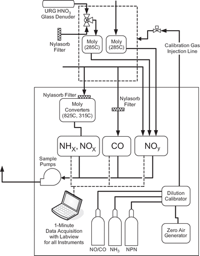
A second chemiluminescence instrument (Teledyne-API, Inc., model 201E) was utilized to determine concentrations for additional nitrogen species (NO_x, NO₂, NH₃, a redundant measurement of NO, and total gas-phase nitrogen species). This three-channel instrument utilized an upstream nylon membrane filter for all channels and at all times to remove particulate material and HNO₃. NO_x measurements via chemiluminescence likely measure some NOy compounds other than NO₂ + NO, as the conversion is nonspecific to NO₂ (Demerjian, 2000; Parrish and Fehsenfeld, 2000; Dunlea et al., 2007). For NH₃ and total gas-phase nitrogen species, a model 501NH converter was used upstream of the NO_x analyzer. Laboratory testing demonstrated that other reduced nitrogen species are also effectively converted to NO in this converter. Ambient air was sampled at the same point in space as the NO_y instrument through an ∼4-m-long, ¼-inch Teflon sampling line. To improve low-level sensitivity, the NH₃/NO_x instrument was retrofitted with a gold-plated reaction cell and pumped with an external high vacuum pump.

A trace-level CO analyzer (Teledyne-API, Inc., model 300EU) was also operated, with a detection limit of <20 ppb. Calibrations for most instruments were performed on an almost daily basis. For NH₃, a calibration was done before, once during, and after the study.

Measurements for the RMNP core site also included detailed observations of fine (PM_2.5) particle composition and coarse (PM₁₀) particle composition, ion size distributions, trace gas concentrations, wet deposition, particle size distributions, particle light scattering, and meteorology. Both time-integrated and high time resolution (at least hourly) measurements were made for nearly all measurement parameters at the core site (Malm et al., 2005).

The Data Set

Species concentrations

Table 2 presents an overall statistical data summary, as well as by season, for a number of parameters measured during the field campaign. PM₁ refers to fine particle mass less than 1.0 µm, derived from the tandem differential mobility analyzer (TDMA) particle size distribution measurements that were made every 15 min. An average particle density of 1.7 g/m³ was assumed (Malm et al., 2005). The data were averaged to 24 hr, and it is the 24-hr statistics that are presented in Table 2. SO₄, NO₃, and NH₄ are the sulfate, nitrate, and ammonium ion concentrations, respectively, collected over a 24-hr period with the URG sampler, while NH_3,urg is the URG denuder measurement of ammonia gas. NH₄B is the ammonium concentration collected on a backup filter, which corresponds to the volatilized ammonia gas from the nylon front filter. It is the sum of NH₄ and NH₄B that corresponds to total particle ammonium. NH_x,gas, NO_x, NO_y, and HNO₃ are the statistical summaries of the 24-hr average NH_x,gas, (NO + NO₂), NO_y—an estimate of all oxidized nitrogen species—and gaseous nitric acid, all derived from the chemiluminescent measurement. NH_x,gas refers to NH₃ + other reduced nitrogen species. Particulate organic matter (POM) is estimated by differencing PM₁ and SO₄ + NO₃ interpreted as being in the fully ammoniated state. Because the TDMA data from which PM₁ and therefore POM are derived have significant periods in which a 15-min sampling interval is missing, the number of valid POM data points reported in Table 2 is often less than for the gaseous species. For the sake of comparison, only statistical summaries for the URG ion data that correspond in time to the POM data are reported. The units of concentration for mass species are in micrograms per cubic meter (µg/m³), while those for gas species are in parts per billion.

Table 2 . Statistical summary of selected PM and gas species concentrations for the entire year as well as seasonally

Variable	Mean	Std dev	Minimum	Maximum	Valid
All
PM1 (µg/m^3)	1.83	1.88	0.13	20.26	185
SO4 (µg/m^3)	0.42	0.28	0.06	2.42	185
NO3 (µg/m^3)	0.15	0.18	0.00	1.48	185
POM (µg/m^3)	1.02	1.61	0.00	17.54	185
NH4 (µg/m^3)	0.13	0.14	0.00	1.01	185
NH4B (µg/m^3)	0.10	0.10	0.00	0.73	185
NHx,gas (ppb)	2.63	1.54	0.17	6.97	336
NH3URG (ppb)	0.45	0.34	0.00	2.51	340
NOx (ppb)	1.32	0.92	0.13	6.85	339
NOy (ppb)	1.53	1.10	0.13	7.64	339
HNO3 (ppb)	0.14	0.13	0.00	0.80	356
Winter
WPM1 (µg/m^3)	0.46	0.60	0.13	3.03	21
WSO4 (µg/m^3)	0.19	0.14	0.06	0.70	21
WNO3 (µg/m^3)	0.08	0.16	0.01	0.78	21
WPOM (µg/m^3)	0.08	0.17	0.00	0.80	21
WNH4 (µg/m^3)	0.05	0.07	0.00	0.32	21
WNH4B (µg/m^3)	0.05	0.09	0.00	0.43	21
NHx,gas (ppb)	1.51	0.69	0.17	4.28	81
NH3URG (ppb)	0.16	0.17	0.00	0.90	88
NOx (ppb)	1.00	0.95	0.16	4.22	82
NOy (ppb)	1.14	1.17	0.16	5.44	82
HNO3 (ppb)	0.08	0.11	0.00	0.58	90
Spring
SPPM1 (µg/m^3)	1.35	0.49	0.56	2.70	20
SPSO4 (µg/m^3)	0.50	0.22	0.17	0.91	20
SPNO3 (µg/m^3)	0.20	0.18	0.03	0.74	20
SPPOM (µg/m^3)	0.33	0.23	0.00	0.78	20
SPNH4 (µg/m^3)	0.16	0.14	0.00	0.43	20
SPNH4B (µg/m^3)	0.16	0.10	0.05	0.39	20
NHx,gas (ppb)	2.84	1.25	0.70	6.52	90
NH3URG (ppb)	0.61	0.45	0.00	2.55	91
NOx (ppb)	1.39	0.98	0.38	4.71	90
NOy (ppb)	1.65	1.17	0.38	6.07	92
HNO3 (ppb)	0.18	0.14	0.00	0.80	93
Summer
SPM1 (µg/m^3)	2.54	2.59	0.40	20.26	68
SSO4 (µg/m^3)	0.45	0.14	0.13	0.96	68
SNO3 (µg/m^3)	0.13	0.15	0.00	1.08	68
SPOM (µg/m^3)	1.74	2.29	0.09	17.54	68
SNH4 (µg/m^3)	0.11	0.08	0.00	0.50	68
SNH4B (µg/m^3)	0.12	0.06	0.00	0.30	68
NHx,gas (ppb)	4.21	1.33	1.58	6.97	84
NH3URG (ppb)	1.05	3.22	0.00	23.83	92
NOx (ppb)	1.36	0.50	0.48	2.79	86
NOy (ppb)	1.62	0.64	0.59	3.32	84
HNO3 (ppb)	0.18	0.12	0.00	0.65	92
Fall
FPM1 (µg/m^3)	1.65	1.09	0.29	4.76	61
FSO4 (µg/m^3)	0.47	0.39	0.09	2.42	61
FNO3 (µg/m^3)	0.18	0.21	0.00	1.48	61
FPOM (µg/m^3)	0.72	0.75	0.05	3.69	61
FNH4 (µg/m^3)	0.18	0.20	0.01	1.01	61
FNH4B (µg/m^3)	0.09	0.12	0.00	0.73	61
NHx,gas (ppb)	1.99	1.16	0.53	5.56	72
NH3URG (ppb)	0.36	0.42	0.00	2.50	71
NOx (ppb)	1.49	0.92	0.34	4.70	72
NOy (ppb)	1.71	1.07	0.36	5.06	72
HNO3 (ppb)	0.12	0.11	0.00	0.52	72
Notes: The data were first averaged to 24 hr and then averaged for the whole year and seasonally. Winter = December, January, February; Spring = March, April, May; Summer = June, July, August; Fall = September, October, November.

As a quality control check, URG sulfate and nitrate ion concentrations were compared to those measured in the IMPROVE program. Concurrently measured sulfate over the same time period showed good agreement, with a comparative R ² = 0.87 and an ordinary least squares (OLS)-derived slope of a scatterplot between the two variables of 0.98 ± 0.02.

Temporal variability of aerosol species

The data in Table 2 are further summarized in Figures 2a and 2b. Figure 2a shows the particulate species average concentrations as an overall average and averages for each season, while Figure 2b presents the same information but for selected measured gas species. On the average, POM makes up about 56% of the fine mass, with sulfates, nitrates, and ammonium contributing on the order of 23%, 8%, and 13%, respectively. All species show seasonal variability, with winter having the lowest concentrations and spring and summer the higher concentrations. PM is highest during the summer at 2.54 µg/m³ and lowest during the winter at 0.46 µg/m³. POM is also highest during the summer months, making up about 70% of PM. On the other hand, sulfates, the second largest contributor to PM, are highest during the fall, when they make up approximately 44% of PM.

Figure 2. (a) Bar plot of measured concentrations of PM_1.0 and the species contributing to PM_1.0 plotted as an overall average and for each season. NH₄B is a measure of the NH₄ volatilized as NH₃ from the NH₃NO₃ collected on the Nylasorb filter. (b) Bar plot of selected gas species plotted as an overall average and as seasonal averages. Concentrations of particle mass are expressed in µg/m³, while gas concentrations are presented in ppb.

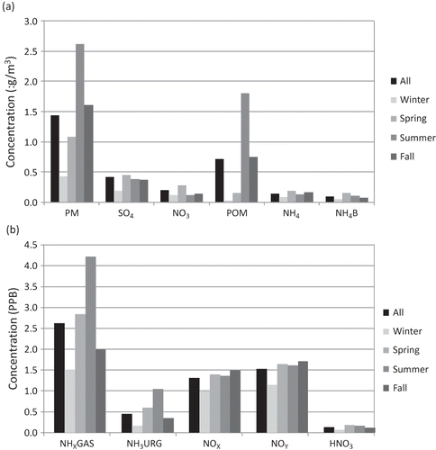
While all particle species show significant variability, NO_x, NO_y, and HNO₃ gas species show little change over the seasons, although winter concentrations are somewhat lower than other seasons. HNO₃ makes up about 12% of NO_y on the average. Also shown in Figure 2 are the average seasonal NH_x,gas and NH₃ concentrations. Remember that NH_x,gas is measured with the modified chemiluminescence instrument, while NH₃ was estimated using a URG sampler fitted with an NH₃ gas denuder. NH_x,gas is a semicontinuous measurement averaged to 24 hr, while the URG is a 24-hr measurement. Both variables have significant seasonal and similar relative cycles, with winter having the lowest concentrations, summer the highest, and spring and fall intermediate concentrations. However, NH_x,gas is about four times greater than NH₃, implying that there are significant levels of reduced nitrogen gases other than NH₃. This topic is discussed at some length later.

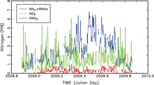
Figure 3 shows a temporal plot of 24-hr average values of NH_x,gas, NO_y, and HNO₃, three variables that are representative of the temporal variability of all measured gaseous species. NO_y and NO_x show very similar temporal variability. Shorter time scale or diurnal variability of gaseous species is discussed in the next section. NH_x,gas exhibits highest concentrations during summer time periods, with higher concentration episodes lasting as long as a week, while during other times of the year episodes are of shorter duration. NO_x and NO_y species are episodic on a shorter time scale than NH_x,gas, and during the summer time frame, the variability between high and low concentrations is significantly less than during other months. As expected, HNO₃ is about a factor of 10 lower than NO_y or NO_x, with summer months being less episodic than other seasons, and is lower during winter and summer months compared to spring and fall.

Figure 3. Temporal plot of chemiluminescence measured concentrations of NH_x,gas, NO_y, and HNO₃.

Diurnal variability

The summer diurnal variability of various aerosol species was explored by first grouping all hourly observations for the summer time period into separate data sets. The median and 10th, 25th, 75th, and 90th percentile concentrations of each group corresponding to each hour of the day were then calculated. These percentile values are presented as box-and-whisker plots for PM₁, NH_x,gas, NO_y, NO_x, temperature, and wind direction in Figure 4. Gaps in the data series correspond to calibration periods. Wind direction was measured on a 10-m tower at the core site in RMNP.

Figure 4. Box-and-whisker plots of measured hourly PM₁, NH₃, NO_y, NO_x, temperature, and wind direction for the summer time period with the median and 10th, 25th, 75th, and 90th percentiles shown.

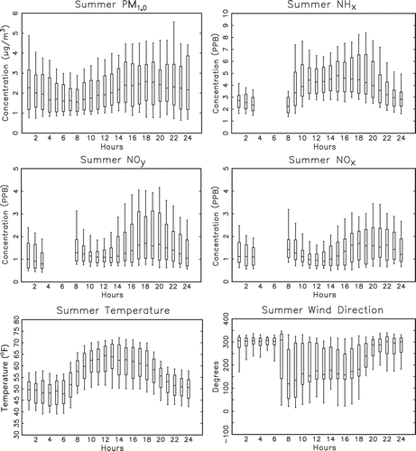
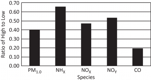
In each box-and-whisker plot there are maximum and minimum median values. The median difference ratio (MDR) is defined as the ratio of the difference between the maximum and minimum median values divided by the maximum median value. Figure 5 is a plot of the median difference ratio for each species. All species exhibit significant diurnal patterns, although the hours at which the maximum and minimum occur are not the same. In general, the concentrations increase uniformly from about 6:00 a.m. (all times MST) to about 3:00 p.m. and then remain elevated throughout the early evening hours. PM₁ reaches its average maximum median value at 6:00 p.m. and its minimum median value at 8:00 a.m.

Figure 5. Median difference ratio for each species shown in Figure 4. The median difference ratio is defined as the ratio of the difference between the hourly maximum and minimum median values divided by the hourly maximum median value.

The increase in NH_x,gas concentrations from an 8:00 a.m. morning low to a secondary maximum at about 11:00 a.m. is quite abrupt. Concentrations then decrease and again increase to reach their maximum level at about 3:00 p.m., decreasing from then until about midnight.

NO_x and NO_y concentrations have afternoon maximums occurring at about 6:00 p.m. and morning minimums at between 10:00 a.m. and 12:00 p.m. Temperature, of course, also has a strong diurnal variation, with morning minimums occurring from 12:00 to 6:00 a.m. and afternoon maximums around noon.

During the evening hours, winds are generally from the northwest, while during daytime from about 7:00 a.m. to 6:00 p.m. winds shift to southeasterly transport, suggesting transport from the Front Range to the receptor site.

Figure 5 shows that NH₃ has the highest or greatest median difference ratio of about 0.65, while NO_x and NO_y are also very high at about 0.50. The median difference ratio for PM₁ is lower but still high at 0.40.

Examples of daily variability of NH_x,gas, NO_y, NO_x, and PM_1.0

Figure 6 is a plot of hourly average species concentrations for various Julian days. Concentrations are in PPB and time is expressed in astronomical time. While Figure 4 shows average diurnal variability of four species, Figure 6 shows examples of specific patterns of diurnal variability of NH_x,gas, NO_x, and NO_y. Figure 6a shows an example in which all three species have similar diurnal patterns, with all species reaching an afternoon/evening maximum at 7:00 p.m. All species having the same diurnal pattern suggests similar transport pathways and possibly similar source regions.

Figure 6. (a)–(f) Hourly average species concentrations of measured NH_x,gas, NO_y, and NO_x for various Julian days; (g) temporal variability of NH_x,gas, NO_y, and PM₁ for Julian Day 309. Concentrations are in ppb and µg/m³, and time is expressed as Julian Day and hours of the day in international time units.

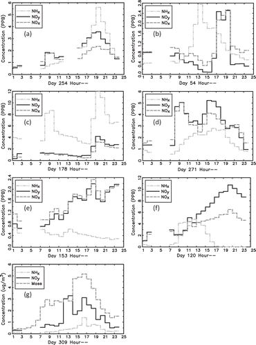
Figures 6b and 6c show more typical patterns in which NH_x,gas concentrations peak before NO_x and NO_y concentrations. Figure 6b shows an example in which the temporal variability of NH_x,gas varies independently from NO_x and NO_y, with NH_x,gas peaking about 4 hr before NO_x and NO_y, suggesting different source regions. Figure 6c shows an interesting example of an NH_x,gas peak in the morning, independent of NO_x and NO_y, while all three species peak together in the evening at about 7:00 p.m.

While NH_x,gas usually reaches its maximum concentration before NO_x and NO_y, and NO_x and NO_y usually have only a single maximum during the day, Figure 6d shows an example of NO_x and NO_y having a morning peak at about 9:00 a.m., followed by an afternoon peak at about 3:00 p.m. NH_x,gas shows very little variability in the morning but similar variability to NO_x and NO_y in the afternoon.

Figure 6e should be compared to Figure 6f. In both cases, NO_x and NO_y increase throughout the day, starting at 7:00 a.m., with the difference being that NO_x and NO_y have similar concentrations on JD = 153, while on JD = 120 NO_x and NO_y concentrations are the same during the morning hours but diverge significantly starting at 11:00 a.m. This divergence continues throughout the day until NO_y concentrations are nearly twice those of NO_x. This of course implies the presence of oxidized nitrogen species other than NO and NO₂ at significant levels. On JD = 153, NH_x,gas decreases throughout the day, while on JD = 120, NH_x,gas concentrations peak around noon.

Finally, Figure 6g, a plot of NH_x,gas, NO_x, and PM₁ (µg/m³), shows that PM₁ also has similar diurnal patterns as gas species. The diurnal cycling of all aerosol species suggests daily cycling of the boundary layer bringing aerosols generated along the Front Range into the park.

Comparison of NH_x,gas chemiluminescence to NH₃ URG measurements

In Table 2, 24-hr average NH_x,gas as measured by chemiluminescence is about a factor of 4–5 greater than 24-hr NH₃ derived from the URG denuder method. NH_x,gas is derived by differencing a chemiluminescence measurement of total nitrogen (TN_x, reduced + oxidized), after passing through a Nylasorb filter, and a modified NO_y measurement. The Nylasorb filter removes particles such as NH₄NO₃ as well as HNO₃ gas. The NO_y instrument does not have a filter in the air stream, so it is responsive to NH₄NO₃ as well as HNO₃. Therefore, to derive an estimate of NH_x,gas that includes HNO₃ and particle NO₃, these two species are added to the difference of the measured TNH_x and NO_y. It is these values that are reported in Table 2.

The straightforward interpretation of NH_x,gas significantly exceeding NH₃ is that there are significant concentrations of reduced nitrogen gas species other than NH₃. However, there are at least two artifacts associated with the NH_x,gas estimate that could lead to an inflated measured concentration. First, the NO_y measurement was made with the molybdenum-catalyzed converter set to 285°C instead of the recommended 315°C, so all oxidized nitrogen may not have been converted, and hence the NO_y is a lower bound estimate of total oxidized nitrogen. Therefore TN_x – NO_y could contain oxidized nitrogen species and be an overestimate of NH_x,gas. Second, the NH_x,gas measurement was made using an airstream with an inline Nylasorb filter. Ammonium nitrate particles collected during lower nighttime temperatures are undoubtedly volatilized during higher daytime temperatures, causing a positive artifact in the NH_x,gas measurement. It can be seen in Table 2 that the backup filter used to measure volatilized ammonium from ammonium nitrate collected on the primary filter in the URG system shows that the concentrations of volatilized ammonium were nearly as high as the ammonium on the primary front filter. These backup filter ammonium concentrations should be indicative of the amount of ammonium volatilized from the inline filter used for the NH_x,gas measurement, depending, of course, on the relative temperature difference between the filter holders for the Nylasorb substrate of the NH_x,gas and the URG system.

If it is assumed that measured NH_x,gas is an overestimation and that NH_x,gas for the most part is primarily NH₃, the NH_x,gas measurements are normalized to the URG measured NH₃ using

(1)

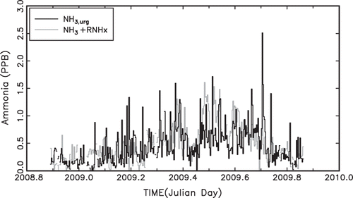
An OLS linear regression solution to eq 1 yields a₁ = 0.25 ± 0.006 and R ² = 0.45. Figure 7 shows a temporal plot of the normalized NH_x,gas and NH_3,urg measurements. For the most part, the agreement between the two measurements is good. There are two or three multiday episodes during the summer when NH_x,gas measurements show elevated concentrations and the NH₃ measurements do not. These are possible cases in which there may be elevated levels of reduced nitrogen other than NH₃ gas.

Figure 7. Temporal plot of NH₃ derived from the URG sampler and the chemiluminescence measurement of NH_x,gas normalized to the URG NH₃ data.

Approach to Apportioning Ammonia to its Emission Sources

The approach taken in this analysis to apportion measured concentrations of various aerosol species at a receptor site to emission sources is to combine modeled transport and dispersion of a conservative tracer released in proportion to emissions with receptor-oriented models to statistically account for removal and chemical processes. From these relationships, the average contributions of source regions throughout North America to the receptor concentration over a period of time are assessed. The goal of the analysis is to separate the contributions from nearby local sources, sources along the Front Range, and other source regions east and west of the Continental Divide.

The tracer modeling system consists of three major components: WRF (Weather Research and Forecasting Model) (Skamarock et al., 2008), a regional weather model; CAMx (Comprehensive Air Quality Model with Extensions) (Environ, 2011), a chemical transport model; and a detailed emission inventory (Adelman and Omary, 2011). WRF (Skamarock et al., 2008) was used to generate hourly meteorological fields on three nested domains of 34 vertical layers and horizontal grid sizes of 36, 12, and 4 km. WRF was initialized with the North American Regional Reanalysis (NARR) data (Mesinger et al., 2006; NARR, 2009). NARR data were also used for analysis nudging on the coarse domain. Data for observational nudging on the 4-km domain were from the Meteorological Assimilation Data Ingest System (MADIS) data set, as well as meteorological data collected as part of RoMANS, including data from a 10-m tower at the core site and a radar wind profiler in Estes Park, CO. Major physics options used in WRF were the rapid radiative transfer model (RRTMG) microphysics (Mlawer et al., 1997), the Kain–Fritsch cumulus parameterization (Kain and Fritsch, 1993; Kain, 2004) on the two coarse domains, the five-layer thermal diffusion land surface model (Dudhia, 1996), and the Yonsei University planetary boundary layer scheme (Hong et al., 2006; Hong and Kim, 2008).

Tracer emissions are based on the ammonia emission inventory developed by the Western Regional Air Partnership (WRAP), the National Emission Inventory (NEI), and are updated to reflect the nested RoMANS model domains and time period (Adelman and Omary, 2011). The major sources within the ammonia emission inventory are livestock operations, agricultural fertilizer applications, and mobile sources.

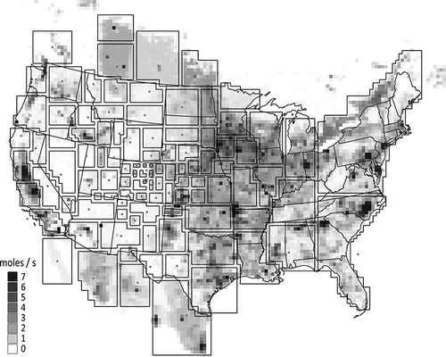
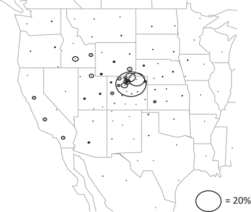
The tracer simulation was conducted using the WRF and ammonia emissions as inputs to CAMx. CAMx is an Eulerian grid air quality model that is often used to investigate regional air pollution. CAMx was modified to simulate an arbitrary number of conserved tracers, with no loss through chemical transformation or deposition. As shown in Figure 8, the inert NH₃ tracer transport simulation was conducted for 107 different source regions throughout North America. The source regions were selected by centering them on high NH₃ emission regions, based on the 2002 WRAP annual average NH₃ emissions inventory. Many areas with little or no NH₃ emissions were excluded. The smallest source regions are near RMNP, and they generally increased in size with distance from the park. Ten source regions were selected within Colorado, including one at RMNP, the neighboring population center at Estes Park, CO, and Denver, CO, as well the agricultural regions in northeastern Colorado.

Figure 8. Source regions and ammonia emission inventory used in the conservative “tracer” analysis.

The receptor model

The starting point for the attribution analysis is the concentrations, C_ki, of modeled ammonia tracer for 1-hr time periods, k, for 107 source areas, i. The bases of most apportionment models rely on the assumption that the concentration of airborne aerosol species can be described by the sum of a number (hopefully, small) of source area vectors. The equation for this description is

(2)

where k = 1...m, the number of observations; i = 1...n, the number of source area patterns contributing to the receptor; j = 1...N, the number of source areas ; C_ki = concentrations of ammonia from source area patterns i for time period k; a_kj = time-weighting functions; S_ji = source vectors; and ϵ_ik = error term including random and lack of fit error.

The source vectors are essentially weighting factors that group source areas together into larger source regions or transport pathways that on the average contribute to elevated concentrations of trace species under certain various, unique types of meteorological conditions.

When source vectors are unknown, it is sometimes possible to gain insight into source–receptor relationships through the use of a singular value decomposition of C_ki (Golub and Reinsch, 1970):

(3)

Comparison of eqs 2 and 3 suggests

(4)

(5)

and

(6)

where s_j = the singular values and u_kj, v_ji = the eigenvectors, m = the number of unique eigenvectors, and ϵ_ik = the error term described earlier.

Therefore, the eigenvectors, v_ji , are the source vectors as derived from the modeled concentrations of ammonia at the receptor site over time. The source vectors, S_ji , are basic patterns found in the modeled data set and are reflective of transport patterns resulting from reoccurring meteorological patterns.

Similar eigenvector analyses have been used where C_ki are measured concentrations of a species of interest, measured at a number of monitoring sites over time to estimate the relative contribution of source regions to measured aerosol levels at the measurement sites. However, in this case, the C_ki are modeled inert concentrations. There are a variety of ways the preceding analysis can be used to approximately apportion the species of interest, in this case ammonia, to the various source regions.

In the following analysis, the eigenvectors are used to group various source regions into larger regions that represent transport from that larger region. These identified groups of source regions are then averaged together for each time period (typically, 1 hr) and treated as independent variables in a regression model where the dependent variables are the measured concentrations of the aerosol of interest and the averaged source regions are the independent variables:

(7)

where NH₃ = the measured hourly or average 24-hr ammonia concentrations, α_jk = the regression coefficients, and Φ_jk = the average of modeled concentrations arriving at the receptor from source areas, grouped according to eigenvectors, v.

A first-order apportionment estimate to easterly and westerly transport

Wind and pollution roses using measured hourly surface wind directions at RMNP can be used to examine the wind direction frequency over the year and the average ammonia concentrations associated with each wind direction (Figure 9). Comparison of the continuous NH₃ to URG values showed a systematic offset of ∼0.6 PPB. Consequently, the continuous data were reduced by this amount. As shown in Figure 9a, the winds were predominantly from a northwestern or southeastern direction. These surface winds are channeled by the local terrain turning the surface winds by ∼60 degrees. If easterly winds are defined as being between 60 to 240 degrees, only 28% of the winds were from the east. However, easterly winds were associated with higher NH₃ concentrations, with an annual average NH₃ of 3 PPB, compared to 1.9 PPB for westerly winds.

Figure 9. (a) Frequency at which the measured surface winds at RMNP are from a given direction and the average NH₃ concentrations associated with each wind direction. (b) Average contributions of the NH₃ concentrations associated with each wind sector to the RMNP annual average NH₃.

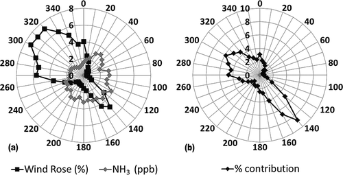
The product of the wind and pollution roses is the contribution of the ammonia for a given wind sector to the average NH₃ and is plotted in Figure 9b as the relative contribution. This gives a semiquantitative estimate of the contributions from sources in a given wind sector. Integration over easterly winds (60–240 degrees) and westerly winds (240–60 degrees) suggests that 44% and 56% of the NH₃ came from sources east and west of RMNP, respectively. The lowest easterly contribution is in the winter at 29% and highest in the fall at 49%. These results are summarized in Table 3. These percentages are likely an upper bound on the contributions from sources east of RMNP. The frequency of easterly winds includes low wind speeds that would contain large local source contributions. In addition, transport from the east often includes trajectories that originate west of RMNP, and therefore, some fraction of the NH₃ concentrations associated with the easterly surface winds will be from sources west of RMNP. This bias is offset by the fact that westerly winds will have contributions from sources east of RMNP. However, this is expected to be relatively small due to the lower frequency of transport from the east.

Table 3 . The estimates of the contribution of sources east and west of RMNP to the seasonal and annual measured NH₃ concentrations

Sources	Winter	Spring	Summer	Fall	Annual
East	29%	44%	45%	49%	44%
West	71%	56%	55%	51%	56%

CAMx modeled concentrations

The CAMx model was run as described in the previous section with the 107 source regions shown in Figure 8 and without deposition and chemistry. A first-order calculation of ammonia lost to deposition was estimated using C*exp(–kt), where C is the modeled inert tracer concentration without deposition, k = v_d/H, where v_d is the deposition velocity and H is the scale height, and t is transport time. Transport time was estimated assuming an average transport velocity of 5 m/sec and an average deposition velocity of 1.0 cm/sec.

Although modeled ammonia concentrations show some diurnal variability on most days and pronounced variability on other days, they do not systematically predict observed diurnal variability of almost all aerosol species on nearly every day that measurements were made. Therefore, in the analysis that follows, 24-hr average concentrations of both modeled and measured concentrations will be used.

Figure 10 is a temporal plot of 24-hr average URG measured and modeled ammonia with estimated deposition, and Table 4 shows the summary statistics for modeled and measured ammonia. Notice that, on the average, modeled and measured ammonia agree surprisingly well in that modeled ammonia is about 50% less than measured. The agreement may be fortuitous, given all the assumptions concerning emission rates, simplifying assumptions concerning deposition, and not having chemistry in the model.

Table 4 . Statistical summary of URG NH₃ and NH₃ estimated from the CAMx tracer data

Variable	Mean	Std dev	Minimum	Maximum	Valid
NH3 (ppb)	0.45	0.34	0.12	2.51	340
Modeled NH3 (ppb)	0.25	0.27	0.07	1.98	340

Figure 10. Time series of measured NH₃ and NH₃ estimated from the CAMx tracer data.

In general, the temporal agreement is also surprisingly good, with an overall correlation between measured and modeled ammonia of 0.37. If the data are averaged to a week, the correlation between measured and modeled is 0.75. For the most part, weekly and seasonal variability is captured by the model.

Table 5 and Figure 11 show modeled relative apportionment of ammonia. “Front Range” refers to the northern front range of the Colorado Rockies, and “northeastern Colorado” refers to regions 184 and 197 in Figure 8. The Front Range and northeastern Colorado include the large confined animal feeding operations (CAFO) around Greeley, Kersey, Fort Morgan, and Brush, Colorado. This region of the United States is predicted to contribute 35% of all measured ammonia at RMNP. Other CAFOs in western Colorado and the Yampa River valley of Colorado also contribute significantly, as does the Snake River basin in southern Idaho, eastern Utah, and as far away as California.

Table 5 . Fractional contribution from various source regions as predicted by the model with simple first-order deposition estimates and by the receptor model

Region	Modeled	Receptor
All CO	0.53	0.51
Outside CO	0.47	0.49
Front Range CO	0.27	0.15
Northeast CO	0.12	0.04
Southeast CO	0.01	0.01
West CO	0.05	0.11
Central CO	0.04	0.14
Yampa	0.04	0.05
Midwest	0.02	0.01
Texas	0.01	0.01
New Mexico	0.01	0.02
Arizona	0.01	0.04
California	0.07	0.12
Snake River	0.06	0.07
Washington state	0.02	0.02
Canada	0.01	0.01
Nebraska	0.03	0.01
Kansas	0.04	0.00
Utah	0.07	0.10
Wyoming	0.05	0.03
Montana	0.02	0.01
Mexico	0.01	0.02

Figure 11. Relative average contributions of various source regions to modeled ammonia at the receptor site. The location of each circle corresponds to the centroid of a source area, while the size of the circle represents the fractional contribution of the source area to the average ammonia concentration at RMNP. The largest circle corresponds to the northern Front Range of Colorado and represents a 27% contribution.

Receptor Model Apportionment of Ammonia

As stated already, the goal of the eigenvector analysis is to identify those groups of source regions that transport to the receptor site during some given time period. The modeled inert tracer concentrations for each source region are normalized to the mean concentration for that site:

(8)

where as before, k = a time index, while j refers to a site.

A singular value decomposition calculation is carried out on the Z_kj matrix. Because the eigenvectors vary to some degree based on the time increment chosen for the eigenvector extraction, the data were broken down on a seasonal basis. Because the first 10 eigenvectors typically explained more than 80% of the variance, they were used in the analysis. After weighting the modeled concentrations for deposition, the sources in each region represented by the eigenvectors were averaged together to form the independent variables in the regression model represented by eq 7.

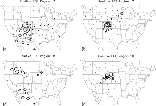
Four typical spatial eigenvectors are shown in Figure 12. The relative sizes of the circles are proportional to the eigenvector weightings, and the center of each circle corresponds to the centroid of the source regions shown in Figure 8. These eigenvectors correspond to typical average transport pathways for the 24-hr averaging time period of the modeled tracer concentrations. Figure 12a corresponds to a general transport pattern from the southwest that includes source areas in western Colorado, Nevada, Arizona, and Mexico. Figure 12b shows more of a stagnant upslope condition with some transport from the Midwest, while 12d also corresponds to an upslope condition but with prior transport from western Colorado, southeastern Wyoming, and western Nebraska. Figure 12c shows transport from the Snake River valley of southern Idaho as well as some transport from the southwest.

Figure 12. Four eigenvectors corresponding to typical transport pathways. Each circle corresponds to a source area, while the size of the circle corresponds to the relative weight of that source area to the eigenvector represented. Transport of emissions from those source areas with the same size circles is correlated in time and therefore is averaged together to represent one large source region.

Because the chemiluminescence estimation of NH_x,gas may contain other reduced species of N than NH₃, both NH_x,gas, as represented by the chemiluminescence measurement, and NH₃, derived from the URG instrument, were used in the regression. However, because the chemiluminescence measurement was normalized to the URG NH₃ data, the relative amount of reduced N species other than NH₃ cannot be inferred. For those cases in which there is a better correlation between NH_x,gas and modeled tracer concentrations than between NH₃ and tracer data, only the possibility of reduced gaseous N species other than NH₃ can be inferred.

The apportionment results corresponding to the model with the highest coefficient of determination, R ², are reported. The results of these regressions are summarized in Table 6, in which a statistical summary of the regression model comparing measured to predicted NH_x,gas concentrations is presented for each season. The first column indicates whether the URG or chemiluminescence data yielded the highest R ². For the spring and fall months, the correlation between chemiluminescence-measured NH_x,gas and tracer data is higher than for URG NH₃, suggesting the presence of some reduced species other than NH₃, or perhaps the chemiluminescence measurement has more precision than the URG measurement. In any case, although not explicitly presented here, the apportionment to source regions is similar for either the URG or chemiluminescence measurement.

Table 6 . Summary statistics for an OLS regression between receptor modeled and measured ammonia concentrations

		R ^2	Slope	Std error	t-Value
URG	Winter	0.49	1.00	0.06	17.55
CHEM	Spring	0.58	1.00	0.04	27.24
URG	Summer	0.21	1.00	0.05	19.97
CHEM	Fall	0.74	1.00	0.05	19.78

Figure 13 shows the time series of model predictions and URG NH₃ or normalized NH_x,gas chemiluminescence data. Concentrations are in PPB. The spring time period, Figure 13b, corresponded to the season with the second highest average concentration, with one 9-day episode exceeding or near the 1.0 PPB concentration level. During this time period, tracer model results compared more favorably with the chemiluminescence measurement because of two factors. First, there are a number of single-day excursions that show up in the URG data but not the chemiluminescence measurements. These excursions are not predicted by the receptor model. Second, during the last quarter of the season, the chemiluminescence measurement showed four days of elevated NH_x,gas significantly above NH₃ levels that were also predicted by the receptor model. This is suggestive of reduced gaseous N species other than NH₃.

Figure 13. Temporal plot of 24-hr average URG NH₃, normalized chemiluminescence (Chem)-derived NH_x,gas, and receptor-modeled normalized NH_x,gas or NH₃, depending on whether the URG or chemiluminescence data were used as the dependent variable in the OLS regression. Each panel represents a season, and the order of the panels is winter, spring, summer, and fall.

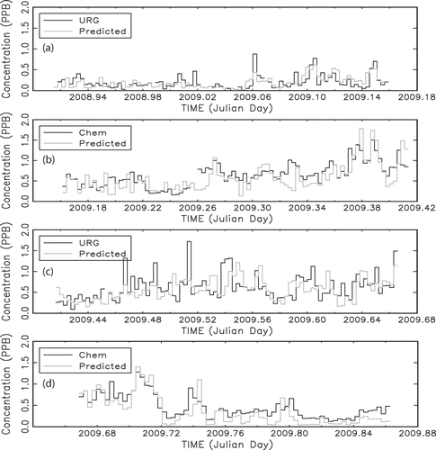
Figure 13c shows the concentration timelines for the summer season. The correspondence between receptor model and measured concentrations is lowest during the summer time period, possibly because of daily mixing of Front Range emissions up to the receptor site that is not fully captured by the WRF windfields. As discussed previously, modeled wind fields are able to capture some vertical mixing associated with diurnal transport but not all. Figure 13d is the concentration timeline for the fall season. It is made up of two episodes in early fall that correspond to transport from the northwest across the Rocky Mountains, northeastern Colorado, and on into the receptor site. The correlation between measurements and the receptor model is highest during this season at over 0.86.

The apportionment estimates are summarized in Table 7 and Figures 14 and 15. Table 7 shows the apportionment of NH_x,gas (primarily NH₃) in PPT to the various source regions for each season of the year, as well as an overall yearly apportionment. The last column is the fraction of NH_x,gas apportioned to each region. The first two rows show the relative apportionment to sources inside and outside Colorado, and the same data are summarized in Figure 14. Overall, there is approximately a 50–50 split of ammonia arriving at the receptor site from inside versus outside Colorado. During the winter, spring, and fall seasons, more ammonia is associated with sources inside Colorado, significantly so during the winter time period. During the summer season, transport from outside Colorado's borders becomes more significant. Averaging across the seasonal averages yields apportionments of about 54% versus 46% from inside and outside of Colorado, respectively. If the inside and outside apportionments are weighted to concentrations, the split is about 51% versus 49%, respectively.

Table 7. Amount of ammonia in PPT apportioned to various source regions as a function of season as well as the average fraction of ammonia apportioned to each source region; also shown is the apportionment to all sources in the state of Colorado

Region	Spring	Summer	Fall	Winter	Average	Fraction
All CO (ppt)	297.14	364.11	198.87	127.65	246.94	0.51
Outside CO (ppt)	285.49	463.41	150.03	68.73	241.91	0.49
Front Range CO (ppt)	81.57	132.40	69.78	11.78	73.88	0.15
Northeast CO (ppt)	34.96	8.28	38.38	1.96	20.89	0.04
Southeast CO (ppt)	5.83	8.28	0.00	0.00	3.53	0.01
West CO (ppt)	40.78	82.75	45.36	53.02	55.48	0.11
Central CO (ppt)	104.87	91.03	38.38	39.28	68.39	0.14
Yampa (ppt)	23.30	49.65	3.49	17.67	23.53	0.05
Midwest (ppt)	5.83	8.28	0.00	0.00	3.53	0.01
Texas (ppt)	0.00	8.28	3.49	0.00	2.94	0.01
New Mexico (ppt)	11.65	16.55	10.47	9.82	12.12	0.02
Arizona (ppt)	17.48	24.83	17.45	15.71	18.86	0.04
California (ppt)	17.48	165.50	52.34	7.86	60.79	0.12
Nevada (LV) (ppt)	0.00	8.28	3.49	0.00	2.94	0.01
Snake River (ppt)	87.39	41.38	10.47	0.00	34.81	0.07
Washington state (ppt)	34.96	8.28	3.49	0.00	11.68	0.02
Canada (ppt)	5.83	0.00	3.49	1.96	2.82	0.01
Nebraska (ppt)	0.00	8.28	3.49	0.00	2.94	0.01
Kansas (ppt)	5.83	0.00	0.00	3.93	2.44	0.00
Oklahoma and Arkansas (ppt)	0.00	0.00	0.00	0.00	0.00	0.00
Utah (ppt)	64.09	82.75	20.93	25.53	48.33	0.10
Wyoming (ppt)	5.83	49.65	10.47	0.00	16.49	0.03
Montana (ppt)	11.65	8.28	3.49	0.00	5.85	0.01
Mexico (ppt)	5.83	24.83	6.98	3.93	10.39	0.02

Figure 14. Fraction of ammonia apportioned to the receptor site from sources in and outside of Colorado as predicted by the hybrid receptor model.

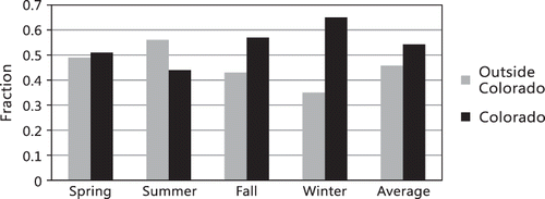
Figure 15. Receptor modeling apportionments of contributions of various source regions to the receptor site as a function of season.

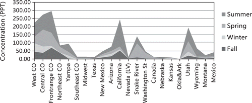
The transport of ammonia to the receptor site is primarily influenced by westerly transport. Although some of the largest emissions of ammonia are found in the Midwest and the eastern part of the United States, these sources apparently contribute little to measured ammonia at the receptor site, while sources to the west are major contributors. This trend is true for all seasons. The source areas outside the borders of Colorado that contribute most to ammonia concentrations are California and northeastern Utah, where there are large CAFO activities. CAFO operations along the Snake River valley in southern Idaho are the next largest out-of-state contributor to ammonia.

Within the state of Colorado, the hybrid receptor modeling results suggest that the Front Range and western and central Colorado all contribute about equally during the spring and summer months, while during the winter season, western and central Colorado contribute more, relative to the Front Range. The Snake River valley is also one of the largest contributors during the spring season. During the fall season, the Front Range and California are the largest contributors, with northeastern, western, and central Colorado contributing slightly less ammonia. Synoptic-scale upslope conditions transported significant amounts of ammonia into the receptor site from CAFO operations along the northern Front Range and northeastern Colorado. These transport conditions were associated with wind trajectories that extended over northeastern Colorado and back across the northwestern United States. Consequently, during these time periods, the Snake River valley, California, and Utah also contributed significantly. During the summer, California contributes significantly, with the Front Range, Utah, and western and central Colorado contributing somewhat less but still quite significantly. The winter season has the western sources contributing most of the measured ammonia.

On the average, northeastern Colorado, including the Front Range, is predicted to contribute about 19% of measured ammonia, with western and central Colorado each contributing 11% and 14%, respectively. The Yampa River valley contributes another 5%.

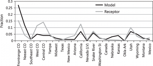
It is informative to compare the receptor modeling results to the tracer CAMx concentrations weighted for deposition. These comparisons are shown in Figure 16. There is an overall general agreement between tracer data weighted for deposition and results of the hybrid receptor model. However, the tracer model suggests about a 39% contribution from the northern Front Range and northeastern Colorado, while the receptor model estimate is below 20%. The receptor model apportions more ammonia to western and central Colorado than does the tracer receptor model. This trend is also true for California and Arizona sources, with the tracer receptor model apportioning about twice as much to these states as the CAMx tracer model.

Figure 16. Receptor modeling apportionment results compared to the apportionment predictions of the tracer CAMx modeled concentrations that have been weighted for dry deposition.

The systematic correlation between diurnally varying local easterly winds measured at the receptor site and diurnal increases in measured NH_x,gas concentrations suggests Front Range transport into the receptor area due to systematic daily mixing of Front Range air into the receptor area. Back-trajectory analysis shows that most transport to the receptor site is a result of transport from the various source areas in the West to the Front Range and then back into the receptor area, carrying both emissions from more distant sources as well as Front Range emissions. Therefore, it is the combination of more distant and local sources along the Front Range ultimately mixing in the receptor area that determines the relative contributions of these sources to nitrogen at the receptor site. Modeled wind fields have to capture not only the westerly transport to the Front Range but also the mixing of these air masses into the park.

The eigenvectors show independent strong correlations between source areas to the west and sources to the northeast but do not capture the systematic daily transport of both pathways into the park. As such, Front Range source regions do not correlate well with individual western source regions and therefore do not fall into transport pathways from the west but into a separate eigenvector. When averaging the source regions represented by the various eigenvectors, Front Range source regions are averaged together. This time series of concentrations is not as well correlated as transport from source regions near and west of the receptor site and therefore do not result in a statistically significant relationship with measured concentration data. Consequently, the receptor modeling results may be an underestimate of the Front Range contribution to NH_x,gas concentrations at the receptor site.

Summary

In Rocky Mountain National Park (RMNP), both wet nitrate deposition and ammonium deposition have increased over the last 20 years. The Rocky Mountain Atmospheric Nitrogen and Sulfur (RoMANS) study was initiated to better understand the origins and physical/chemical characteristics of nitrogen species, as well as the complex chemistry occurring during transport from source to receptor. Increases in ammonia emissions tend to increase and change the composition of particulate matter (PM) mass concentrations. Regardless of the chemical form and phase of the nitrogen, it will ultimately be deposited onto terrestrial or aquatic surfaces. However, where these species are deposited does depend on the chemical form and phase of the nitrogen. For example, gaseous ammonia has higher deposition rates and will deposit closer to the sources, while ammoniated particulates can be transported hundreds of kilometers before deposition.

As part of the study, a monitoring program was initiated for one year starting in November 2008. The monitoring program consisted of intensive, high time resolution measurements of particles, gas, wet deposition, and meteorology at a core site in RMNP.

Gas-phase measurements were made continuously and in real time, with 1-min averaged data. Instruments were collocated with the existing IMPROVE and CASTNET sites near the eastern boundary of RMNP. Continuous measurements included an estimation of nitric acid (HNO₃), reduced nitrogen gaseous species including ammonia (NH_x,gas), nitrogen oxides (NO_x), NO_y compounds (NO_x plus other reactive oxidized nitrogen species), and carbon monoxide (CO). Calibrations for most instruments were performed on an almost daily basis. For NH_x,gas, a calibration was done before, once during, and after the study.

The approach taken in this analysis to apportion emission sources to measured concentrations of various aerosol species at a receptor site combines modeled transport and dispersion of a conservative tracer released in proportion to ammonia emissions, with receptor-oriented models to statistically account for removal and chemical processes. From these relationships the average contributions of source regions throughout North America to the receptor concentration over a period of time were assessed. The goal of the analysis is to separate out the contributions from nearby local sources, sources along the Front Range, and other source regions east and west of the Continental Divide.

The tracer modeling system consists of three major components: WRF (Weather Research and Forecasting Model; Skamarock et al., 2008), a regional weather model; CAMx (Comprehensive Air Quality Model with Extensions; Environ, 2011), a chemical transport model, and a detailed emission inventory (Adelman and Omary, 2011). WRF (Skamarock et al., 2008) was used to generate hourly meteorological fields on three nested domains of 34 vertical layers and horizontal grid sizes of 36, 12, and 4 km. Data for observational nudging on the 4-km domain were from the Meteorological Assimilation Data Ingest System (MADIS) data set, as well as meteorological data collected as part of RoMANS, including data from a 10-m tower at the core site and a radar wind profiler in Estes Park, CO.

A spatial eigenvector analysis of modeled tracer data was used to group various source regions into larger regions that represent transport from that larger region. These identified groups of source regions were then averaged together for each time period and treated as independent variables in a regression model in which the dependent variables are the measured concentrations of the aerosol of interest and the averaged source regions are the independent variables.

All gaseous species show pronounced diurnal variability throughout the year. Typically, minimum concentrations occur during evening hours and maximums in the late afternoon. NH₃ has the highest or greatest median difference ratio of about 0.65, while NO_x and NO_y are also very high at about 0.50. The median difference ratio for PM₁ is lower but still high at 0.40.

In some cases use of NH_x,gas in the receptor model yielded higher correlations and variance explained than did URG data, suggesting either sources of reduced nitrogen other than ammonia or possibly that the chemiluminescence measurement has a higher precision than the URG measurement. The relative apportionment between sources is approximately the same whether URG or chemiluminescence measurements are used.

Two objectives of the study were to develop an approximate understanding of the relative contributions of ammonia sources in and outside the state of Colorado to measured reduced gaseous ammonia species in RMNP and to assess whether large ammonia emissions in the agricultural area of the midwestern portion of the United States contributed significantly to ammonia in RMNP. In answer to the first question, the analysis suggests that slightly more ammonia measured at RMNP originates from in-state sources. However, within in the uncertainty of the apportionment methodology, it is fair to say that there is about a 50–50 split between in-state and out-of-state sources.

Regarding the second question, it seems pretty clear that very little of measured ammonia at the receptor site had its origins in the Midwest. The model suggests that no more than about 10% of measured ammonia originates from sources east of eastern Colorado (102.3º longitude).

Sources west of Colorado contribute on the order of 30% of measured ammonia, with California contributing on the order of 13%, eastern Utah contributing 10%, and the Snake River valley of southern Idaho 7%.

The systematic correlation between diurnally varying, local easterly winds measured at the receptor site and diurnal cycling of all aerosol species concentrations suggests Front Range transport into the receptor area.

The inability of the WRF modeled winds to faithfully reproduce these systematic diurnal patterns suggests that the receptor model may be underestimating the contribution of Front Range and northeastern Colorado ammonia emissions. With that said, the receptor model suggests that within the state of Colorado, on the average about an equal amount of ammonia is coming from western and central Colorado and the Front Range, including the Greeley area, at about 10–15%. Northeastern Colorado is estimated to contribute another 4%. The Yampa River valley is estimated to contribute about 5%.

Concentrations of ammonia are highest during the summer months, when the northern Front Range of Colorado and California, along with western and central Colorado and Utah, have the largest contributions. During the spring season, the Front Range, central Colorado, the Snake River valley, and Utah contribute most of the ammonia, while during the fall season, the Front Range plus northeastern Colorado are the largest contributors to ammonia, with California and western and central Colorado also contributing significantly. The winter season corresponds to the lowest measured concentrations, and source regions are primarily more local, but Utah and Arizona sources contribute at times.

Acknowledgment

This work was funded by the National Park Service under contract H2370094000. The assumptions, findings, conclusions, judgments, and views presented herein are those of the authors and should not be interpreted as necessarily representing the National Park Service policies.

References

- Adelman , Z. and Omary , M. 2011 . Emissions Modeling Final Report—Developing 2009 Emissions for the NPS-ARD RoMANS Study, Phase 2 , Chapel Hill , NC : Institute for the Environment, University of North Carolina .
- Bai , H.L. and Wen , H.Y. 2000 . Performance of the annular denuder system with different arrangements for HNO3 and HNO2 measurements in Taiwan . J. Air Waste Manage. Assoc. , 50 ( 1 ) : 125 – 30 . doi: 10.1080/10473289.2000. 10463991
- Baron , J.S. , Rueth , H.M. , Wolfe , A.N. , Nydick , K.R. , Allstott , E.J. , Minear , J.T. and Moraska , B. 2000 . Ecosystem responses to nitrogen deposition in the Colorado Front Range . Ecosystems , 3 : 352 – 68 . doi: 10.1007/s100210000032
- Baron , J.S. , Driscoll , T.C. , Stoddard , J.L. and Richer , E.E. 2011 . Empirical critical loads of atmospheric nitrogen deposition for nutrient enrichment and acidification of sensitive U.S. lakes . BioScience , 61 ( 8 ) : 602 – 13 . doi: 10.1525/bio.2011.61.8.6
- Blett, T., and K. Morris. 2004. Nitrogen Deposition: Issues and effects in Rocky Mountain National Park. Technical background document. http://www.cdphe.state.co.us/ap/rmnp/noxtech.pdf (http://www.cdphe.state.co.us/ap/rmnp/noxtech.pdf)
- Burns , D.A. 2003 . Atmospheric nitrogen deposition in the Rocky Mountains of Colorado and southern Wyoming—A review and new analysis of past study results . Atmos. Environ. , 37 : 921 – 32 . doi: 10.1016/S1352-2310(02)00993-7
- Campbell , D.H. , Baron , J.S. , Tonnessen , K.A. , Brooks , P.D. and Schuster , P.F. 2000 . Controls on nitrogen flux in alpine/subalpine watersheds of Colorado . Water Resources Res. , 36 : 37 – 47 . doi: 10.1029/1999WR900283
- Campbell , D.H. , Kendall , C. , Chang , C.C.Y. , Silva , S.R. and Tonnessen , K.A. 2002 . Pathways for nitrate release from an alpine watershed: Determination using delta N-15 and delta O-18 . Water Resources Res. , 38 doi: 10.1029/2001WR00294
- CASTNET . 2010 . Annual Report , Washington , DC : U.S. Environmental Protection Agency .
- Demerjian , K.L. 2000 . A review of national monitoring networks in North America . Atmos. Environ. , 34 ( 12–14 ) : 1861 – 84 . doi: 10.1016/S1352-2310(99)00452-5
- Dudhia , J. 1996 . “ A multi-layer soil temperature model for MM5 ” . In Proceedings of the 6th PSU/NCAR Mesoscale Model Users’ Workshop , 49 – 50 . Boulder , CO : National Center for Atmospheric Research .
- Dunlea , E.J. , Herndon , S.C. , Nelson , D.D. , Volkamer , R.M. , San Martini , F. , Sheehy , P.M. , Zahniser , M.S. , Shorter , J.H. , Wormhoudt , J.C. , Lamb , B.K. , Allwine , E.J. , Gaffney , J.S. , Marley , N.A. , Grutter , M. , Marquez , C. , Blanco , S. , Cardenas , B. , Retama , A. , Villegas , C.R.R. , Kolb , C.E. , Molina , L.T. and Molina , M.J. 2007 . Evaluation of nitrogen dioxide chemiluminescence monitors in a polluted urban environment . Atmos. Chem. Phys. , 7 ( 10 ) : 2691 – 704 . doi: 10.5194/acp-7-2691-2007
- ENVIRON . 2011 . CAMx User's Guide Version 5.30 , Novato , CA : ENVIRON International Corp .
- Fehsenfeld , F.C. , Dickerson , R.R. , Hubler , G. , Luke , W.T. , Nunnermacker , L.J. , Williams , E.J. , Roberts , J.M. , Calvert , J.G. , Curran , C.M. , Delany , A.C. , Eubank , C.S. , Fahey , D.W. , Fried , A. , Gandrud , B.W. , Langford , A.O. , Murphy , P.C. , Norton , R.B. , Pickering , K.E. and Ridley , B.A. 1987 . A ground-based intercomparison of NO, NOx, and NOy measurement techniques . J. Geophys. Res. Atmos. , 92 ( D12 ) : 14710 – 22 . doi: 10.1029/JD092iD12p14710
- Fontijn , A. , Sabadell , A.J. and Ronco , R.J. 1970 . Homogeneous chemiluminescent measurement of nitric oxide with ozone—Implications for continuous selective monitoring of gaseous pollutants . Anal. Chem. , 42 ( 6 ) doi: 10.1021/ac60288a034
- Galloway , J.N. , Likens , G.E. , Keene , W.C. and Miller , J.M. 1982 . The composition of precipitation in remote areas of the world . J. Geophys. Res. , 87 : 8771 – 76 . doi: 10.1029/JC087iC11p08771
- Galloway , J.N. , Schlesinger , W.H. , Levy , H. , Michaels , A. and Schnoor , J.L. 1995 . Nitrogen fixation: Atmospheric enhancement—Environmental response . Global Biogeochem. Cycles , 9 : 235 – 52 . doi: 10.1029/95GB00158
- Golub , G.H. and Reinsch , C. 1970 . Singular value decomposition and least squares solutions . Numer. Math. , 14 : 403 – 20 . doi: 10.1007/BF02163027
- Hand , J.L. , Copeland , S.A. , Day , D.E. , Dillner , A.M. , Indresand , H. , Malm , W.C. , McDade , C.E. , Moore , C.T. Jr , Pitchford , M.L. , Schichtel , B.A. and Watson , J.G. 2011 . Spatial and seasonal patterns and temporal variability of haze and its constituents in the United States , Fort Collins , CO : Cooperative Institute for Research in the Atmosphere, Colorado State University .
- Hedin , L.O. , Armesto , J.J. and Johnson , A.H. 1995 . Patterns of nutrient loss from unpolluted, old-growth temperate forests: Evaluation of biogeochemical theory . Ecology , 76 : 493 – 509 . doi: 10.2307/1941208
- Hong, S.-Y., and S.-W. Kim. 2008. Stable boundary layer mixing in a vertical diffusion scheme. In Proc. Ninth Annual WRF User's Workshop. Boulder, CO: National Center for Atmospheric Research. http://www.mmm.ucar.edu/wrf/users/workshops/WS2008/abstracts/3-03.pdf (http://www.mmm.ucar.edu/wrf/users/workshops/WS2008/abstracts/3-03.pdf)
- Hong , S.-Y. , Noh , Y. and Dudhia , J. 2006 . A new vertical diffusion package with explicit treatment of entrainment processes . Monthly Weather Rev. , 134 : 2318 – 41 . doi: 10.1175/MWR3199.1
- Kain , J.S. 2004 . The Kain-Fritsch convective parameterization: An update . J. Appl. Meteorol. , 43 : 170 – 81 . doi: 10.1175/1520-0450(2004)043<0170:TKCPAU>2.0.CO;2
- Kain , J.S. and Fritsch , J.M. 1993 . “ Convective parameterization for mesoscale models: The Kain–Fritch scheme ” . In The Representation of Cumulus Convection in Numerical Models , Edited by: Emanuel , K.A. and Raymond , D.J. 165–170. Boston, MA: American Meteorological Society .
- Lehmann , C.M.B. , Bowersox , V.C. and Larson , S.M. 2005 . Spatial and temporal trends of precipitation chemistry in the United States . Environ. Pollut. , 135 : 347 – 61 . doi: 10.1016/j.envpol.2004.11.016
- Malm , W.C. , Day , D.E. , Kreidenweis , S. , Collett , J.L. Jr , Carrico , C.M. , McMeeking , G.R. , Lee , T. , Carrillo , J. and Schichtel , B.A. 2005 . Hygroscopic properties of an organic-laden aerosol . Atmos. Environ. , 39 : 4969 – 82 . doi: 10.1016/j.atmosenv.2005.05.014
- Mesinger , F. , DiMego , G. , Kalnay , E. , Mitchell , K. , Shafran , P.C. , Ebisuzaki , W. , Jovic , D. , Woollen , J. , Rogers , E. , Berberry , E.H. , Ek , M.B. , Fan , Y. , Grumbine , R. , Higgins , W. , Li , H. , Lin , Y. , Manikin , G. , Parrish , D.D. and Shi , W. 2006 . North American regional reanalysis . Bull. Am. Meteorol. Soc. , 87 : 343 – 60 . doi: 10.1175/BAMS-87-3-343
- Mlawer , E.J. , Taubman , S.J. , Brown , P.D. , Iacono , M.J. and Clough , S.A. 1997 . Radiative transfer for inhomogeneous atmospheres: RRTM, a validated correlated-k model for the longwave . J. Geophys. Res. , 102 ( 14 ) : 16663 – 82 . doi: 10.1029/97JD00237
- North American Regional Reanalysis. 2009. Home page. (accessed 2009) http://wwwt.emc.ncep.noaa.gov/mmb/rreanl/index.html (http://wwwt.emc.ncep.noaa.gov/mmb/rreanl/index.html)
- Parrish , D.D. and Fehsenfeld , F.C. 2000 . Methods for gas-phase measurements of ozone, ozone precursors and aerosol precursors . Atmos. Environ. , 34 ( 12–14 ) : 1921 – 57 . doi: 10.1016/S1352-2310(99)00454-9
- Rueth , H.M. and Baron , J.S. 2002 . Differences in Englemann spruce forest biogeochemistry east and west of the Continental Divide . Ecosystems , 5 : 45 – 57 . doi: 10.1007/s10021-001-0054-8
- Seinfeld , J.H. and Pandis , S.N. 1998 . Atmospheric Chemistry and Physics: From Air Pollution to Climate Change , New York , NY : John Wiley .
- Skamarock , W.C. , Klemp , J.B. , Dudhia , J. , Gill , D. , Barker , D. , Duda , M.G. , Huang , X.Y. , Wang , W. and Powers , J.G. 2008 . A Description of the Advanced Research WRF Version 3 , NCAR Technical Note, NCAR/TN-475+STR . Boulder, CO: National Center for Atmospheric Research (NCAR).
- Williams , E.J. , Baumann , K. , Roberts , J.M. , Bertman , S.B. , Norton , R.B. , Fehsenfeld , F.C. , Springston , S.R. , Nunnermacker , L.J. , Newman , L. , Olszyna , K. , Meagher , J. , Hartsell , B. , Edgerton , E. , Pearson , J.R. and Rodgers , M.O. 1998 . Intercomparison of ground-based NOy measurement techniques . J. Geophys. Res. Atmos. , 103 ( D17 ) : 22261 – 80 . doi: 10.1029/98JD00074