Statistical evaluation of a new air dispersion model against AERMOD using the Prairie Grass data set

Abstract

In this work, the authors present a statistical assessment of two atmospheric dispersion models. One of them, AERMOD (American Meteorological Society/Environmental Protection Agency Regulatory Model), adopted by the U.S. Environmental Protection Agency, is widely used in many countries and here is taken as a baseline to assess the performance of a newly proposed model, MODELAR (Modelo Regulatório de Qualidade do Ar). In terms of parameterizations and modeling options, MODELAR is a somewhat simple model. It is currently being considered for adoption as the regulatory model in Paraná State, Brazil. The well-known Prairie Grass data set, already used in earlier evaluations of the same version of AERMOD analyzed here, was used to perform model assessment. The evaluations employed well-established statistical performance descriptors and techniques. The results indicate that MODELAR is a slightly better predictor, for the Prairie Grass data set, of concentrations under unstable conditions, whereas AERMOD has a better performance under near-neutral and stable conditions. Moreover, cases of severe overestimation and underestimation, as detected by the Factor of Two index, are clearly associated with extreme stability conditions (both unstable and stable), stressing the need for better parameterizations under these conditions.

Implications:

Statistical evaluation of a proposed numerical dispersion model, called MODELAR, and of the well-established dispersion model AERMOD was performed, using the Prairie Grass data set as reference. The results showed that MODELAR performs well under unstable conditions, making it competitive with other dispersion models. However, the results also showed that both models require improvement of the dispersion parameterizations for extreme stability conditions, both unstable and stable.

Introduction

In this work, we present a new dispersion model that is under development as a candidate for the regulatory air dispersion model of Paraná State, Brazil. Given the widespread use of U.S. Environmental Protection Agency (EPA) models in Brazil for licensing purposes, the new model is compared against EPA's AERMOD (American Meteorological Society/Environmental Protection Agency Regulatory Model; Cimorelli et al., 2004a) using a commonly used data set for dispersion model evaluation (Prairie Grass; Barad, 1958). Both the Prairie Grass data set and the AERMOD simulation results used in this work were obtained by the work of Olesen et al. (2007).

Most regulatory atmospheric dispersion models in use are based on gaussian approximations. A basic assumption of those models is that wind speed and turbulence diffusion coefficients are constant to produce a gaussian concentration distribution about the plume's centerline with lateral and vertical standard deviations and , respectively, which are usually estimated from meteorological data (Hanna et al., 1982; Tirabassi, 1989).

Such gaussian models have the advantage of being analytical, easy to implement and apply, and have performed reasonably well in several field experiments where they were put to test (Weil and Jepsen, 1977; Harrison and Mac Cartney, 1980). However, in their original form they failed to consider the mean wind variation with height and the nonhomogeneity of turbulence. It has been recognized since the 1960s that these simplifications are inadequate in applications where the wind speed varies considerably with height, or in conditions close to local free convection (Gifford, 1968; Pasquill, 1974).

In an effort to address these shortcomings, several studies were developed to include the effects of mean wind and turbulent diffusion dependence with height (Demuth, 1978; Huang, 1979; Lin and Hildemann, 1996). The resulting family of analytical models includes the current regulatory models in use by the EPA, the AERMOD modeling system (Cimorelli et al., 2004a) and CALPUFF modeling system (Scire et al., 2000).

However, although there are many turbulence and wind parameterizations that show reasonable agreement with observational data (Ulke, 2000; Demuth, 1978; Huang, 1979; Lin and Hildemann, 1996), analytical models use simpler approximations of these profiles to obtain exact solutions, such as AERMOD, whose concentration formulations consider these profiles by an equivalent (effective) value constructed by averaging over the layer through which plume material travels directly from the source to receptor (Cimorelli et al., 2004b).

In this work, in an effort to overcome those simplifications inherent to some analytical solutions, the dependence with height of the mean wind and turbulent diffusivity is represented explicitly in a numerical solution of the advection-diffusion equation. The model has reached a stage where a first operational version is available for initial tests. The operational version includes the ability to incorporate an arbitrary number of sources at different heights, and to spread a two-dimensional (2D) solution laterally with a gaussian plume, using the same strategy of the models AERMOD (Cimorelli et al., 2004b) and OML (Operationelle Meteorologiske Luftkvalitetsmodeller) (Olesen et al., 2007), but (unlike them) without inclusion of the meander effect. In this paper, only the 2D version without lateral spreading, and with a source located close to the ground, is used, since this is enough for comparison with the Prairie Grass data.

The evaluation of the performance of the resulting Eulerian numerical model, called MODELAR (Modelo Regulatório de Qualidade do Ar), as well as its comparison with AERMOD, are the central objectives of this paper. As a first step towards establishing MODELAR's capacity to predict pollutant concentrations with a skill comparable to models widely used in Brazil for regulatory purposes, we compare both MODELAR and AERMOD against the Prairie Grass data set.

Prairie Grass is considered a standard database for atmospheric dispersion model validation (American Society for Testing and Materials [ASTM], 2000). With the Prairie Grass data set, it is possible to evaluate the model performance in predicting the field concentration emitted continually over flat terrain, near the ground and near the source.

The criteria used here to assess the model's skill follow the recommendations in “Standard Guide for Statistical Evaluation of Atmospheric Dispersion Model Performance” (ASTM, 2010) and Chang and Hanna (2004). Model evaluation is performed independently of wind direction, and only vertical dispersion is taken into account, with all measured concentrations averaged laterally.

In Description of Model MODELAR and Description of Model AERMOD, we briefly describe the relevant aspects of AERMOD and MODELAR for this work. In sections The Prairie Grass Experiment and Comparisons Criteria, we describe in more detail both the data set and statistical measures of model performance, respectively. In Results, we give the main results of the comparisons between models and data. Then, we summarize the results and conclude the work in Conclusion.

Description of Model MODELAR

MODELAR solves the advection-diffusion equation numerically, neglecting longitudinal diffusion, aligning the x-axis with the mean wind direction, and the z-axis with the vertical direction. The resulting differential equation is the same as solved by Wortmann et al. (2005):

(1)

where is the vertical turbulent diffusion coefficient.

The numerical solution employs an implicit trapezoidal method, which allows relative large grid spacing in x. The horizontal grid spacing is constant in x. The grid points in the vertical are unevenly distributed, with smaller spacing close to the ground where velocity and concentration gradients are larger.

The solution proceeds column-wise (in the z-direction) from the first column for , i.e., for positive x values. Each column is solved with the successive overrelaxation iterative method. The iterations stop when the relative error in concentration is smaller than 10⁻¹⁰.

Zero-flux boundary conditions are prescribed at the bottom () and top () of the domain, viz.,

(2)

at both heights.

For unstable conditions, the vertical turbulent diffusion is the same as used by Velho et al. (1997):

(3)

where

(4)

is the convective velocity scale, h is the height of the atmospheric boundary layer, is the mean virtual potential temperature, and is the surface kinematic virtual sensible heat flux. Reynold's separation is written with the overbar indicating the mean and the lowercase letter the turbulent fluctuation.

For stable conditions, the turbulence is characterized by local values, such as the local Monin-Obukhov length (Degrazia and Moraes, 1992):

(5)

where L is the Monin-Obukhov length calculated with surface flux values. For a shear-dominated stable boundary layer, = 1.5 and  = 1.0 (Nieuwstadt, 1984). Furthermore, there is a local velocity scale given by

(6)

in which = 1.5 and is the friction velocity at surface (Wyngaard et al., 1974).

The vertical turbulent diffusion for stable or neutral conditions is the same as used by Degrazia et al. (2000):

(7)

where f is the Coriolis parameter.

Description of Model AERMOD

AERMOD model 04300 was used in this work; this is the same version used by Olesen et al. (2007), whose description is given by Cimorelli et al. (2004a).

Essentially, AERMOD solves eq 1, but with a constant wind speed and turbulent diffusion coefficient. These values, however, are calculated from mean values of the corresponding profiles predicted by similarity theory, for the centerline of the plume down to the receptor. They are called “effective” parameters, and denoted here by a tilde, e.g., and .

The general expression for the calculation of AERMOD's concentrations is

(8)

where Q is the source emission rate, is the effective wind speed, and P _y and are probability density functions that describe the lateral and vertical concentration distributions, respectively.

Under stable conditions, the plume is represented by gaussian distributions both in the horizontal and vertical directions. Under unstable conditions, the horizontal distribution remains gaussian, whereas the vertical distribution is bigaussian, in order to better represent the asymmetrical effect of positive and negative vertical velocity fluctuations.

Furthermore, in the unstable boundary layer, AERMOD uses two additional sources to describe the pollutant's distribution from the actual source: an “indirect” source to address the lofting behavior and dispersion of “nonpenetrating” plumes, and a “penetrated” source to account for plume material that initially penetrates the inversion but subsequently fumigates into the CBL (Convective Boundary Layer). In addition, image sources are included to satisfy the zero flux conditions at .

The vertical concentration distributions of the indirect and actual sources are bigaussian, and the vertical concentration distribution of the penetrated source is gaussian. Regarding the distribution of the actual source, the vertical dispersion in the unstable surface layer is parameterized according to so as to provide good agreement between the modeled and observed concentrations from the Prairie Grass experiment (Cimorelli et al., 2004b).

The Prairie Grass Experiment

The data used in this work come from the Prairie Grass experiment, which took place near O'Neil, Nebraska, during the summer of 1956. The site altitude is 596.37 m and its location is 42°29.6′N, 98°34.3′W (Barad, 1958).

Sixty-eight releases “(runs)” were made under different stability conditions. For each run, SO₂ tracer was continuously released without buoyancy from a height of 0.46 m above ground, except four runs 65, 66, 67, and 68, whose release height was 1.5 m. Concentration measurements were made by receptors placed at 1.5 m above ground and in arcs at 50, 100, 200, 400, and 800 m from the source, and the averaging time of the observed concentration values was 10 min. Simultaneous measurements of wind and temperature profiles in the surface layer, and radiosoundings, are also available.

From the measured velocity and temperature profiles in the surface layer, Olesen et al. (2007) estimated a roughness length of 6 mm. For runs 3, 4, 13, and 14, during which the wind speed was below 1 m sec⁻¹, a much larger roughness of 10 cm was obtained. We will follow the common practice of excluding these runs from model evaluations using the Prairie Grass data set.

There is not an official digital source of the Prairie Grass data set, but it can be obtained from http://www.dmu.dk/International/Air/Models/Background/oml.htm. This is a digital annex to the work by Olesen et al. (2007). The data set includes for each 10-min run: friction velocity (u_*0), boundary-layer height (h), Monin-Obukhov length (L), and convective velocity scale (w_*). A constant momentum roughness () is adopted. Also provided at that Web site are computed values of the crosswind integrated concentration values both from the observed data and from modeling results for AERMOD version 04300. These are the same data as used by Marie et al. (2012) and Sharan and Kumar (2009).

Comparison Criteria

We compare model simulations with observed concentrations using a set of statistical scores. First, several indices defined in Olesen (2001) are used:

(9)

(10)

(11)

(12)

Fa2 = Fraction of data that satisfy

(13)

where NMSE is the normalized mean square error, GM is the geometric mean bias, GV is the geometric variance, Fa2 is the Factor of Two, and FB is the fractional bias. The overbar indicates means over the runs. In eqs 9– 13, are the observed crosswind integrated concentrations, and are their counterparts predicted by the model. The best results for a model are GM, GV, Fa2 = 1.0, and FB, NMSE = 0.0.

The indices defined above should be considered as a whole, as they obviously address different kinds of errors, such as bias (in the case of FB, GM) and dispersion (in the case of NMSE, GV). Moreover, it is well known that all averages can be heavily influenced by the presence of outliers (Hanna et al., 2004).

Chang and Hanna (2004) established criteria for a good dispersion model, based on eqs 9– 13, namely Fa2 > 0.5, −0.3< FB < 0.3, 0.7 < GM < 1.3, NMSE < 0.5, and GV < 1.6.

Due to the short averaging time of the Prairie Grass observations (10 min), we are providing comparisons of observed and simulated crosswind integrated concentration values. This allows evaluation of model performance for vertical dispersion. This also avoids having to deal with problems associated with the horizontal dispersion, which is a strong function of averaging time, especially for averaging times of 1 hr or less. We use a ratio:

(14)

to assess the relative difference in the crosswind integrated values as a function of downwind distance and stability.

In order to assess whether the performance statistics for the two models are significantly different, we are using bootstrap resampling to compare those statistics based on Student's t test with a 90% level of confidence, as recommended by ASTM (2010).

In order to do that, we generated bootstrap samples composed of the observed values and the associated simulation results for both models, respecting the “concurrent sampling” recommended by ASTM (2010). In our case, around 500 resamplings with replacement were utilized, and the statistics given by eqs 9– 12 were calculated separately for stable and unstable runs. Each bootstrapped sample size was 33 runs × 5 arcs for unstable, and 30 runs × 5 arcs for stable conditions, the same values of the experiment.

Each bootstrapped sample generates a difference Δ between the performance statistics for the two models. We compute the average and standard deviation (σ_Δ) to obtain the t value, . When t is larger than 1.645, it is possible to conclude with 90% of confidence that there is a significant difference between the two models for the particular statistic being tested.

Results

Following ASTM (2010), the data are assessed separately for unstable (L < 0) and stable (L > 0) conditions. In Figure 1a and b we show the results of observed versus predicted crosswind integrated concentrations values for MODELAR and AERMOD, respectively, for unstable conditions. Then, in Figure 2a and b results are shown for stable conditions.

Figure 1. Scatterplots of simulated by MODELAR (a) and AERMOD (b) against observed in the Prairie Grass experiment, in unstable conditions.

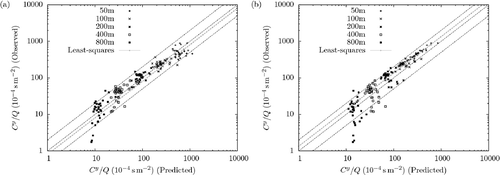
Figure 2. Scatterplots of simulated by MODELAR (a) and AERMOD (b) against observed in the Prairie Grass experiment, in stable conditions.

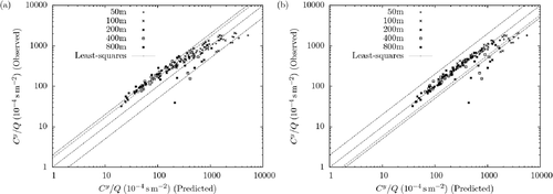
Note in Figures 1 and 2 three dotted lines, which are , , and , going from bottom to top. Furthermore, we plotted the lines of least-squares fits forced to intercept the origin of the graph (on the linear scale) to see quickly whether the model is over or underestimating the observations.

As expected, for unstable conditions the highest observed and predicted concentrations occur at the arc closest to the source (50 m), whereas for stable conditions the largest concentrations are more spread out along the 50-, 100-, and 200-m arcs.

A key feature of Figures 1–2 is that MODELAR has a tendency for underestimating the vertical dispersion under unstable conditions, the opposite occurring with AERMOD. For stable conditions, MODELAR has a tendency for overestimating and AERMOD for underestimating the vertical dispersion. Furthermore, with regards to the direct comparison of the observed and predicted concentrations, those estimates exceeding a factor of 2 are all overestimates for AERMOD, whereas for MODELAR there are both over- and underestimates of the observed concentrations.

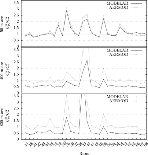
A wider comparison between predicted and observed concentrations consists of the scores given by eqs 9– 13 and by the so-called residual plots (Hanna et al., 2004). For unstable conditions, they are shown in Table 1 and in Figure 3, and for stable conditions in Table 2 and in Figure 4.

Table 1. Results of model performance statistics under unstable conditions

Arc	Model	NMSE	FA2	FB	GM	VG
50 m	MODELAR	0.16	0.94	0.20	1.24	1.16
	AERMOD	0.11	1.0	−0.33	0.71	1.14
100 m	MODELAR	0.10	0.97	0.04	1.02	1.07
	AERMOD	0.15	1.0	−0.34	0.70	1.19
200 m	MODELAR	0.09	0.97	−0.15	0.85	1.09
	AERMOD	0.27	0.91	−0.31	0.74	1.28
400 m	MODELAR	0.15	0.94	−0.21	0.86	1.20
	AERMOD	0.30	0.76	−0.16	0.92	1.38
800 m	MODELAR	0.31	0.76	−0.21	0.98	1.47
	AERMOD	0.43	0.67	0.01	1.25	1.89
Mean	MODELAR	0.16	0.91	−0.07	0.99	1.20
	AERMOD	0.25	0.87	−0.23	0.86	1.38
All data	MODELAR	0.15	0.92	0.10	0.98	1.19
	AERMOD	0.13	0.87	−031	0.84	1.35

Figure 3. Residual plot of against run number for an unstable atmosphere, for the 50-, 200-, and 400-m arcs.

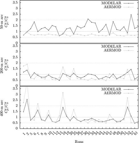
Table 2. Results of model performance statistics under stable conditions

Arc	Model	NMSE	FA2	FB	GM	VG
50 m	MODELAR	0.41	0.87	0.30	1.14	1.14
	AERMOD	0.55	0.87	0.39	1.20	1.20
100 m	MODELAR	0.11	1.0	−0.07	0.82	1.13
	AERMOD	0.23	0.93	0.20	1.02	1.12
200 m	MODELAR	0.13	0.97	−0.25	0.68	1.27
	AERMOD	0.22	0.93	0.20	1.02	1.12
400 m	MODELAR	0.21	0.70	−0.34	0.62	1.45
	AERMOD	0.28	0.93	0.26	1.10	1.20
800 m	MODELAR	0.46	0.47	−0.38	0.60	1.72
	AERMOD	0.54	0.87	0.33	1.22	1.39
Mean	MODELAR	0.26	0.80	−0.15	0.77	1.34
	AERMOD	0.36	0.91	0.28	1.10	1.20
All data	MODELAR	0.30	0.80	0.03	0.75	1.33
	AERMOD	0.41	0.91	0.29	1.11	1.20

Figure 4. Residual plots of against run number for a stable atmosphere, for the 50-, 400-, and 800-m arcs.

For unstable conditions, we find that the mean value of all scores are slightly better for MODELAR than for AERMOD and that they satisfy the quality criteria suggested by Chang and Hanna (2004), reviewed in section Comparison Criteria.

In these conditions, MODELAR overestimates C ^y for the 50- and 100-m arcs, and underestimates C ^y for 200 through 800 m. Although on average MODELAR looks unbiased, there is a clear variation in the bias as a function of distance. This implies that MODELAR is underestimating the vertical dispersion for the 50- and 100-m arcs, and is overestimating the vertical dispersion for 200–800 m downwind.

On the other hand, AERMOD underestimates C ^y under unstable conditions initially, with a definite trend in the bias with distance, so that by 800 m it is overestimating C ^y. This implies that AERMOD is overestimating the vertical dispersion until the 800-m arc. In that arc, AERMOD underestimates the vertical dispersion.

Although the unstable surface layer parameterization used by AERMOD was designed to provide good agreement between the modeled and observed concentrations from the Prairie Grass experiment, it is noticeable in Figure 3 and Table 1 that the AERMOD predictions worsens with distance. Nieuwstadt (1980) and Weil et al. (2012) suggest a weaker dependence of vertical dispersion, σ_z, with the distance in unstable conditions and within the convective matching region. Then, it is possible that changing the x ² dependence in to a power law might improve AERMOD's predictions. However, this was not tested, since modifying AERMOD was not the focus of this work.

For stable conditions, AERMOD overestimates C ^y for the 50-, 400-, and 800-m arcs, and is nearly perfect for the 100- and 200-m arcs, whereas MODELAR underestimates C ^y, starting at 100-m arc onwards. Thus, MODELAR increasingly overestimates the vertical dispersion as the distance downwind increases.

Table 3 presents the statistics computed over bootstrap resampling. The values of the MODELAR and AERMOD statistics for both unstable and stable conditions are listed, together with the difference and the t statistic. Interestingly, for all statistics except NMSE under unstable conditions, the tests show that the model's performances are significantly different. Thus, for unstable conditions, MODELAR is better in terms of FB, MG, and VG. For stable conditions, on the other hand, MODELAR is better for NMSE and FB, and AERMOD is better for MG and VG.

Table 3. Model statistics, mean difference, and by bootstrap resampling

	Unstable				Stable
Parameter	MODELAR	AERMOD		t	MODELAR	AERMOD		t
NMSE	0.15	0.13	0.02	0.56	0.29	0.40	−0.11	−4.42
FB	0.10	−0.31	0.41	9.00	0.02	0.28	−0.30	−10.82
MG	0.98	0.84	0.14	4.83	0.75	1.11	−0.36	−18.15
VG	1.19	1.35	−0.16	−4.48	1.33	1.20	0.13	2.65
Note: The critical value is 1.645.

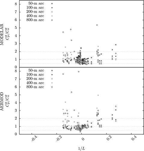
It is also important to look closely at the cases where the models errors are largest: both in Figures 3 and 4 we can see that some runs overestimate by a factor of 2 or larger. We now turn our attention to these cases and try to detect possible connections with atmospheric stability. Thus, is plotted against the 1/L in Figure 5. Clearly, the largest overestimations occur for very unstable and for very stable conditions, i.e., for the smallest values of Monin-Obukhov length.

Figure 5. Residual plot of against 1/L.

Conclusion

We performed a comparison of two models, AERMOD and MODELAR, using the Prairie Grass Project data set. As usual, the data were analyzed separately for unstable and stable conditions. Further specific analyses to highlight different model capabilities were then conducted.

From our comparisons of observed and simulated crosswind integrated concentration values, we see that, under unstable conditions, MODELAR is underestimating the vertical dispersion for the 50-m arc; it is overestimating the vertical dispersion for 200–400 m downwind, and it is nearly perfect on the other arcs. Under unstable conditions, AERMOD is overestimating the vertical dispersion initially, but when it reaches the 800-m arc it underestimates vertical dispersion. Under stable conditions, AERMOD behaves better than MODELAR because MODELAR tends to overestimate the vertical dispersion starting at the100-m arc onwards.

In order to assess the quality of the predictions as a function of distance from the source, we used residual plots for all runs in each measuring arc, as well as standard statistics for model performance: NMSE, GM, GV, Fa2, and FB (for definitions, see section Comparison Criteria). Furthermore, using the Student's t test based on bootstrap resampling, we compared the performance statistics between the models: they are significantly different (in a statistical sense) most of the time, with MODELAR being better under unstable conditions. For stable conditions, MODELAR “wins’’ in NMSE and FB, and AERMOD in MG and VG.

The Fa2 (Factor of Two) results show several predictions in excess of 200%, or less than 50%, of the observed values. Residual analysis of the data shows that these extreme overestimates/underestimates are systematically related either to very stable or very unstable conditions, where the Monin-Obukhov Theory does not perform well. These results indicate the need for better parameterization of the dispersion parameters under those conditions.

Acknowledgment

The authors thank the suggestions by three reviewers, which helped to improve this work considerably.

Funding

This work was partially supported by IAP (Instituto Ambiental do Paraná) through research project FUNPAR 2629, and by the Federal University of Paraná through the Graduate School and the Graduate Program of Environmental Engineering (UFPR/PRPPG/PPGEA).

References

- American Society for Testing and Materials . 2010 . Standard Guide for Statistical Evaluation of Atmospheric Dispersion Model Performance , West Conshohocken, PA: American Society for Testing and Materials .
- Barad , M.L. 1958 . Project Prairie Grass, A Field Program in Diffusion. Geophysical Research , Vol. 59 , I.Report AFCRC-TR-58-235(I). Bedford, MA: Air Force Cambridge Research Center .
- Chang , J.C. and Hanna , S.R. 2004 . Air quality model performance evaluation . Meteorol. Atmos. Phys , 87 : 167 – 196 . doi: 10.1007/s00703-003-0070-7
- Cimorelli , A.J. , Perry , S.G. , Venkatram , A. , Weil , J.C. , Paine , R.J. , Wilson , R.B. , Lee , R.F. , Peters , W.D. and Brode , R.W. 2004a . AERMOD: A dispersion model for industrial source applications. Part I: General model formulation and boundary layer characterization . J. Appl. Meterol , 44 : 682 – 693 .
- Cimorelli , A.J. , Perry , S.G. , Venkatram , A. , Weil , J.C. , Paine , R.J. , Wilson , R.B. , Lee , R.F. , Peters , W.D. , Brode , R.W. and Paumier , J.O. 2004b . AERMOD: Description of Model Formulation , U.S. Environmental Protection Agency . Research Triangle Park, NC
- Cox , W.M. and Tikvart , J.A. 1990 . A statistical procedure for determining the best performing air quality simulation model . Atmos. Environ , 24A:2387–2395
- Degrazia , G.A. , Anfossi , D. , Carvalho , J., C., M. , Tirabassi , T. and Campos Velho , H. 2000 . Turbulence parameterization for PBL dispersion models in all stability conditions . Atmos. Environ , 34 : 3575 – 3583 . doi: 10.1016/S1352-2310(00)00116-3
- Degrazia , G.A. and Moraes , O. 1992 . A model for eddy diffusivity in a stable boundary layer . Boundary Layer Meteorol , 58 : 205 – 214 . doi: 10.1007/BF02033824
- Demuth . 1978 . A Contribution the analytical to steady solution of the diffusion equation for line sources . Atmos. Environ , 12 : 1255 – 1258 .
- Dresser , A.L. and Huizer , R.D. 2011 . CALPUFF and AERMOD model validation study in the near field: Martins Creek revisited . J. Air Waste Manage. Assoc , 61 : 647 – 659 . doi: 10.3155/1047-3289.61.6.647
- Gifford , F.A. 1968 . “ An outline of theories of diffusion in the lower layers of the atmosphere ” . In Meteorology and Atomic Energy , Edited by: Slade , D.H. 65 – 116 . Washington , DC : U.S. Department of Energy .
- Hanna , S.R. , Briggs , G.A. and Hosker , R.P. 1982 . Handbook on Atmospheric Diffusion , Washington , DC : Technical Information Center, U.S. Department of Energy .
- Hanna , S.R. , Hansen , O.R. and Dharmavaram , S. 2004 . FLACS CFD air quality model performance evaluation with Kit Fox, MUST, Prairie Grass, and EMU observations . Atmos. Environ , 38 : 4675 – 4687 . doi: 10.1016/j.atmosenv.2004.05.041
- Harrison , R.M. and MacCartney , H.A. 1980 . A comparison of the predictions of a simple gaussian plume dispersion model with measurements of pollutant concentration at ground-level and aloft . Atmos. Environ , 14 : 589 – 596 .
- Huang , C.H. 1979 . A theory of dispersion in turbulent shear flow . Atmos. Environ , 13 : 453 – 463 .
- Lin , J.-S. and Hildemann , L.M. 1996 . Analytical solutions of the atmospheric diffusion equation with multiple sources and height-dependent wind speed and eddy diffusivities . Atmos. Environ , 30 : 239 – 254 . doi: 10.1016/1352-2310(95)00287-9
- Marie , E.E.J. , Hubert , B.-B. G. and Pierre , O.A. 2012 . A First-order WKB approximation for air pollutants dispersion equation . Atmos. Res , 120– 121 : 162 – 169 .
- Nieuwstadt , F. 1980 . Application of mixed-layer similarity to the observed dispersion from a ground-level source . J. Appl. Meteorol , 19 : 157 – 162 .
- Nieuwstadt , F. 1984 . The turbulent structure of the stable nocturnal boundary layer . J. Atmos. Sci , 41 : 2202 – 2216 . doi: 10.1175/1520-0469(1984)041<2202: TTSOTS>2.0.CO;2
- Olesen , H. 2001 . “ Ten years of harmonization activities ” . In Past, present, and future. Presented at the 7th International Conference on Harmonization within Atmospheric Dispersion Modelling for Regulatory Purposes, Belgirate, Italy, May 28--31
- Olesen , H.R. , Berkowicz , R. and Lofstrom , P. 2007 . Evaluation of OML and AERMOD , Aarhus, Denmark: National Environmental Research Institute .
- Pasquill , F. 1974 . Atmospheric Diffusion , New York, NY: Ellis Horwood Ltd .
- Scire, J.S., Robe, F.R., Fernau, M.E.Yamartino, R.J. 2000. A User's Guide for the CALMET Meteorological Model (Version 5). Concord, MA: Earth Tech, Incaccessed August 2013 http://www.src.com/calpuff/download/CALPUFF_UsersGuide.pdf (http://www.src.com/calpuff/download/CALPUFF_UsersGuide.pdf)
- Sharan , M. and Kumar , P. 2009 . An analytical model for crosswind integrated concentrations released from a continuous source in a finite atmospheric boundary layer . Atmos. Environ , 43 : 2268 – 2277 . doi: 10.1016/j.atmosenv.2009.01.035
- Tirabassi , T. 1989 . Analytical air pollution advection and diffusion models . Water Air Soil Pollut , 47 : 19 – 24 . doi: 10.1007/BF00468993
- Ulke , A.G. 2000 . New turbulent parameterization for a dispersion model in the atmospheric boundary layer . Atmos. Environ , 34 : 1029 – 1042 . doi: 10.1016/S1352-2310(99)00378-7
- U.S. Environmental Protection Agency . 2003 . AERMOD: Latest Features and Evaluation Results , U.S. Environmental Protection Agency . EPA-454/R-03-003. Research Triangle Park, NC
- Velho , H.F.C. , Carvalho , J.C. and Degrazia , G.A. 1997 . Nonlocal exchange coefficients for the convective boundary layer derived from spectral properties . Atmos. Phys , 70 : 57 – 64 .
- Weil , J.C. and Jepsen , A.F. 1977 . Evaluation of the gaussian plume model at the Dickerson Power Plant . Atmos. Environ , 11 : 901 – 910 .
- Weil , J.C. , Sullivan , P.P. , Patton , E.G. and Moeng , C. 2012 . Statistical variability of dispersion in the convective boundary layer: Ensembles of simulations and observations . Boundary Layer Meteorol , 145 : 185 – 210 . doi: 10.1007/s10546-012-9704-y
- Wortmann , S. , Vilhena , M. , Moreira , D.M. and Buske , D. 2005. A new analytical approach to simulate the pollutant dispersion in the PBL. Atmos. . Environ , 39 2171 – 2178 . doi: 10.1016/j.atmosenv.2005.01.003
- Wyngaard , J.C. , Cote , O. and Rao , K.S. 1974 . Modeling of the Atmospheric Boundary Layer. Advances in Geophysics , San Diego : Academic Press . 18A