Comparative statistical study of hourly precipitation determined by radar-based Stage IV and ground-based methods in the North Central United States

Abstract

Detailed hourly precipitation data are required for long-range modeling of dispersion and wet deposition of particulate matter and water-soluble pollutants using the CALPUFF model. In sparsely populated areas such as the north central United States, ground-based precipitation measurement stations may be too widely spaced to offer a complete and accurate spatial representation of hourly precipitation within a modeling domain. The availability of remotely sensed precipitation data by satellite and the National Weather Service array of next-generation radars (NEXRAD) deployed nationally provide an opportunity to improve on the paucity of data for these areas. Before adopting a new method of precipitation estimation in a modeling protocol, it should be compared with the ground-based precipitation measurements, which are currently relied upon for modeling purposes. This paper presents a statistical comparison between hourly precipitation measurements for the years 2006 through 2008 at 25 ground-based stations in the north central United States and radar-based precipitation measurements available from the National Center for Environmental Predictions (NCEP) as Stage IV data at the nearest grid cell to each selected precipitation station. It was found that the statistical agreement between the two methods depends strongly on whether the ground-based hourly precipitation is measured to within 0.1 in/hr or to within 0.01 in/hr. The results of the statistical comparison indicate that it would be more accurate to use gridded Stage IV precipitation data in a gridded dispersion model for a long-range simulation, than to rely on precipitation data interpolated between widely scattered rain gauges.

Implications:

The current reliance on ground-based rain gauges for precipitation events and hourly data for modeling of dispersion and wet deposition of particulate matter and water-soluble pollutants results in potentially large discontinuity in data coverage and the need to extrapolate data between monitoring stations. The use of radar-based precipitation data, which is available for the entire continental United States and nearby areas, would resolve these data gaps and provide a complete and accurate spatial representation of hourly precipitation within a large modeling domain.

Introduction

Long-range air pollution transport and deposition models are used to assess the impact of distant emission sources for regulatory applications, including air quality impact assessments and Air Quality Related Values (AQRVs), under the Prevention of Significant Deterioration program. In order to model accurately the long-range effects of emissions of particulate matter and water-soluble pollutants to the atmosphere, atmospheric dispersion models such as CALPUFF must take into account absorption of pollutants into rainwater, and wet deposition onto the ground. This requires input to the dispersion model of hourly precipitation data over long periods of time (such as one or several years) for the modeling domain, which for long-range modeling analyses can be an extensive geographical area. The currently accepted air dispersion modeling protocol for the evaluation of wet deposition, consideration of precipitation in atmospheric pollutant chemistry and effect on visibility or other AQRVs relies on the use of precipitation data from rain gauges. In sparsely populated areas such as the north central United States, ground-based continuous precipitation measurement stations mostly using tipping bucket rain gauges are widely and not uniformly spaced, thus resulting in poor spatial representation and disparate resolution of the data input to the dispersion models. The availability of remotely sensed precipitation data by satellite and the National Weather Service (NWS) array of next-generation radars (NEXRAD) deployed nationally provide an opportunity to improve on the paucity of data for these areas. These data resources are currently used or considered for input to watershed, hydrological, and ecological models (Sexton et al., 2010; Wang and Wolf, 2009; Zhang and Srinivasan, 2010). The same challenges of sparsely and randomly located precipitation measurements are faced by the atmospheric dispersion modeling community, and although the current modeling protocol does not include use of these alternate data sources, it is prudent to investigate their potential use. The objective of the study from which this paper is derived was to evaluate the feasibility and appropriateness of using hourly NEXRAD precipitation data as input for a long-range atmospheric transport dispersion analysis.

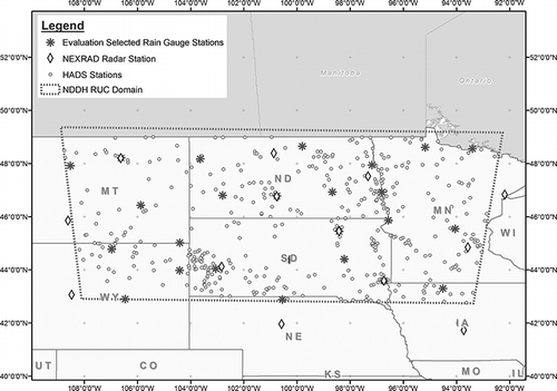
In an effort to address the paucity of data within the modeling domain of interest in the north central United States for use in the CALPUFF long-range dispersion model, a methodology has been developed that relies on the use of hourly precipitation data available from the National Center for Environmental Predictions (NCEP), which are derived from analyses of NEXRAD Doppler radar data, satellite data, and automated precipitation monitoring stations. The resulting database, referred to as Stage IV precipitation data, was used to extract the needed precipitation data for a representative CALPUFF modeling domain. The modeling domain of interest is shown in Figure 1.

Figure 1. Spatial distribution of HADS stations, NEXRAD radar stations, and selected precipitation stations.

However, once the data were extracted, there was some concern regarding the representativeness and validity of the hourly Stage IV precipitation data. Therefore, a statistical data validation plan was developed and implemented to compare the Stage IV hourly data with measured rain gauge data. The statistical analysis plan included comparison of 3 yr of hourly data at 25 selected monitoring stations, as described in this paper. It is important to note that the sites were selected to obtain spatial representation of the modeling domain, but were not initially screened for instrument precision.

To the authors’ knowledge, the proposed use of NEXRAD-derived data in dispersion models, which have traditionally used rain gauge data, is new. Evaluations and validation studies of NEXRAD-derived precipitation data compared with rain gauge data have been performed by others provide insight in the short-term and long-term, i.e., minutes to hourly periods and monthly to annual periods, respectively, data comparisons (Habib et al., 2009; Over et al., 2007; Sexton et al., 2010; Wang and Wolf, 2009; Young et al., 2000; Zhang and Srinivasan, 2010). The results from the statistical analysis presented in this study are consistent with these prior evaluations. The statistical analyses performed indicate good correlation between the NEXRAD-derived and high-resolution rain gauge data. An interesting and important finding of the study is that rain gauge data from lower precision instruments are not representative of short-term precipitation periods and should not be used in atmospheric dispersion modeling analyses.

Rain gauge precipitation data

The rain gauge is the primary instrument used to measure precipitation at most primary and secondary observing stations. Hourly precipitation data are archived and available from the National Climatic Data Center (NCDC) in the TD3240 data format. At automated precipitation measurement stations managed by NWS that use tipping bucket rain gauges, precipitation accumulates until a preset amount of liquid is obtained, then the rain gauge “trips” and is emptied. The number of “trips” during an hour is multiplied by the amount required to trip the gauge to obtain the hourly precipitation rate in inches per hour. High-precision rain gauges “trip” when 0.01 in accumulates in the rain gauge, but other “low-precision” rain gauges need a 0.1-in accumulation to “trip.”

For a period of several consecutive hours of light precipitation (<0.1 in/hr), a high-precision rain gauge would record the precipitation during each hour to the nearest 0.01 in, but a low-precision rain gauge would record zero precipitation for several hours until 0.1 in accumulates in the rain gauge, then the gauge would “trip” and record 0.1 in/hr during the last hour. The input of data from low-precision rain gauges into dispersion models can lead to errors in wet deposition of pollutants, because wet deposition would actually occur during all hours of light precipitation (small raindrops have a high surface area for pollutant absorption), not only for the last hour during which the rain gauge tripped and recorded 0.1 in/hr of rain. The hourly precipitation measurements used in the analysis discussed in this paper were obtained from the NCDC and are referred to as the TD3240 precipitation data.

Stage IV radar-based precipitation data

NCEP developed a method, called Stage IV, of estimating hourly precipitation data for a grid covering the continental United States, where each grid point is the center of a 4 km × 4 km square. The Stage IV data are developed from an analysis of

•	Rain gauge reports from 1450 Automated Surface Observing Stations (ASOS) (NWS, 2005)
•	About 5500 Hydrometeorological Automated Data System (HADS) rain gauges (NWS, 2012)
•	Precipitation estimates from 160 NEXRAD Doppler radar sites

Stage IV precipitation data (NCEP, 2012) for the period considered in this analysis are calculated using an optimal estimation algorithm called the Multi-Sensor Precipitation Estimator (MPE), in a four-stage process, as follows:

•	Stage I is an hourly digital precipitation (HDP) estimate derived from reflectivity measurements from a single NEXRAD radar site after the application of several quality control algorithms.
•	Stage II is the single-radar-site HDP product merged with nearby surface rain gauge observations with a mean field bias correction applied using a Kalman filter algorithm.
•	In Stage III, the Stage II rainfall data from multiple weather radars covering an entire river forecast center (RFC) are combined using the MPE-selected estimate for each Hydrologic Rainfall Analysis Project (HRAP) grid point. Stage III at the RFC is initially run automatically, then quality-controlled by a human analyst.
•	Stage IV consists of grouping the Stage III rainfall data from each of the RFCs into a single data set covering the entire continental United States.

The output is generated on the HRAP grid, a polar stereographic projection with 1121 × 881 grid points, whose y-axis is parallel to the meridian at 105°W longitude. The grid covers the entire continental United States, and portions of Canada, Mexico, and the Atlantic and Pacific Oceans.

Stage IV precipitation data (NCEP, 2012) are archived as gridded binary (GRIB) files, which contain the date and time and hourly precipitation rates at each grid point in millimeters per hour. The precision of Stage IV precipitation is 0.01 in/hr (0.254 mm/hr).

Methods and Materials

For this study, 25 precipitation stations were selected from the TD3240 hourly precipitation data set to represent the modeling domain shown in Figure 1 covering North Dakota, South Dakota, and parts of neighboring states. Table 1 lists the 25 precipitation stations selected for this statistical study and their corresponding location and other relevant details. It was determined through a review of site-specific equipment that precipitation was measured to a precision of 0.01 in/hr at 18 of the 25 stations, and to a precision of 0.1 in/hr at seven stations.

Table 1. Selected rain gauge precipitation stations for the comparative analyses

			Precision			Longitude		Latitude			Data Completeness, %
Station Number	City	State	0.1 in	0.01 in	Gauge Type*	Deg	Min	Deg	Min	Elevation (m)	2006	2007	2008
137058	Ringsted	IA	X		FPR-E	−94	31	43	18	372	100.00	82.11	97.71
211250	Camp Norris	MN	X		FPU	−95	11	48	37	393	67.11	90.96	72.48
214026	International Falls	MN		X	AWPAG	−93	24	48	34	361	100.00	83.52	0.00
217294	Saint Cloud	MN		X	AWPAG	−94	03	45	33	310	100.00	100.00	99.91
218947	White Rock Dam	MN	X		FPR-D	−96	34	45	52	312	98.87	97.15	87.31
240165	Alzada	MT	X		FPR-D	−104	25	45	01	1052	91.83	24.97	65.50
243558	Glasgow	MT		X	AWPAG	−106	37	48	13	697	99.43	100.00	100.00
245690	Miles City	MT		X	AHTB	−105	53	46	26	800	99.46	99.90	100.00
249900	Zortman	MT	X		FPR-D	−108	32	47	55	1231	91.01	87.77	93.46
258760	Valentine	NE		X	TB	−100	33	42	53	789	100.00	100.00	97.81
320819	Bismarck	ND		X	AHTB	−100	45	46	47	503	100.00	100.00	100.00
322183	Th. Roosevelt AP	ND		X	AHTB	−102	48	46	48	786	99.98	100.00	99.90
322859	Fargo	ND		X	TB	−96	49	46	56	274	100.00	99.71	99.87
323616	Grand Forks	ND		X	TB	−97	11	47	57	257	100.00	100.00	100.00
324413	Jamestown	ND		X	AHTB	−98	40	46	56	455	100.00	100.00	100.00
327655	Rolette	ND	X		FPR-E	−99	48	48	38	494	96.44	91.87	95.89
329425	Williston	ND		X	TB	−103	38	48	10	580	99.68	100.00	100.00
390020	Aberdeen	SD		X	AWPAG	−98	25	45	27	395	99.95	100.00	100.00
394127	Huron	SD		X	AWPAG	−98	13	44	24	390	99.97	100.00	99.92
396597	Pierre	SD		X	AHTB	−100	17	44	23	531	99.89	100.00	100.00
396937	Rapid City	SD		X	AHTB	−103	03	44	03	963	99.57	100.00	99.77
397667	Sioux Falls	SD		X	FPR-E	−96	44	43	35	436	93.89	99.23	97.77
481570	Casper	WY		X	AWPAG	−106	28	42	54	1627	99.69	99.90	98.80
486935	Osage	WY	X		FPU	−104	25	43	59	1317	86.79	91.74	54.09
488155	Sheridan	WY		X	AWPAG	−106	58	44	46	1202	99.45	100.00	99.81
Notes: *Gauge types: tipping bucket (TB), automated heating tipping bucket (AHTB), all-weather precipitation accumulation gauge (AWPAG), Fischer-Porter Rebuild–Sutron (FPR-D), Fischer-Porter Rebuild–CES (FPR-E), and Fischer-Porter Upgrade (FPU).

Hourly precipitation data in TD3240 format for each of the 25 stations were obtained for the years 2006, 2007, and 2008 from the National Climatic Data Center Web site (NCDC, 2013), and loaded into spreadsheets as a function of date and local standard time. Software was developed that would determine coordinates of the HRAP grid cell nearest to each of the above stations, and extract hourly Stage IV precipitation data from the GRIB files for each hour. These data were adjusted for time zone, and loaded into the spreadsheets for comparison with the simultaneous TD3240 precipitation data. The Stage IV method is based mainly on radar measurements at NEXRAD radar sites, which are generally spaced hundreds of kilometers apart. The 25 precipitation stations evaluated for this study were located at various distances from the nearest NEXRAD radar site, including four stations within 2 km of a radar site, three stations more than 200 km from the nearest radar site, and 13 stations between 100 and 200 km from the nearest radar site. Table 2 presents the name, location, and distance of the nearest NEXRAD radar site for the 25 precipitation measurement stations evaluated in this study.

Table 2. Location and distance of nearest NEXRAD radar site to rain gauge stations

Rain Gauge Station				Nearest NEXRAD Radar Station
City	State	Latitude°N	Longitude°W	City	State	Latitude°N	Longitude°W	Distance(km)
Ringsted	IA	43.30	94.52	Des Moines	IA	41.73	93.72	186
Camp Norris	MN	48.62	95.18	Fargo/Grand Forks	ND	47.53	97.33	200
International Falls	MN	48.57	93.40	Duluth	MN	46.84	92.18	213
Saint Cloud	MN	45.55	94.05	Minneapolis	MN	44.85	93.57	87
White Rock Dam	MN	45.87	96.57	Fargo/Grand Forks	ND	47.53	97.33	193
Alzada	MT	45.02	104.42	Rapid City	SD	44.13	102.83	160
Glasgow	MT	48.22	106.62	Glasgow	MT	48.21	106.62	1.3
Miles City	MT	46.43	105.88	Glasgow	MT	48.21	106.62	205
Zortman	MT	47.92	108.53	Glasgow	MT	48.21	106.62	145
Valentine	NE	42.88	100.55	North Platte	NE	41.96	100.58	103
Bismarck	ND	46.78	100.75	Bismarck	ND	46.77	100.76	1.6
Th. Roosevelt AP	ND	46.80	102.80	Bismarck	ND	46.77	100.76	155
Fargo	ND	46.93	96.82	Fargo/Grand Forks	ND	47.53	97.33	76
Grand Forks	ND	47.95	97.18	Fargo/Grand Forks	ND	47.53	97.33	48
Jamestown	ND	46.93	98.67	Fargo/Grand Forks	ND	47.53	97.33	121
Rolette	ND	48.63	99.80	Minot AFB	ND	48.39	100.86	83
Williston	ND	48.17	103.63	Minot AFB	ND	48.39	100.86	206
Aberdeen	SD	45.45	98.42	Aberdeen	SD	45.46	98.41	0.7
Huron	SD	44.40	98.22	Aberdeen	SD	45.46	98.41	118
Pierre	SD	44.38	100.28	Aberdeen	SD	45.46	98.41	189
Rapid City	SD	44.05	103.05	Rapid City	SD	44.13	102.83	19
Sioux Falls	SD	43.58	96.73	Sioux Falls	SD	43.59	96.73	0.6
Casper	WY	42.90	106.47	Riverton	WY	43.07	108.48	164
Osage	WY	43.98	104.42	Rapid City	SD	44.13	102.83	128
Sheridan	WY	44.77	106.97	Billings	MT	45.86	108.61	176

Statistical analysis procedure

The purpose of the statistical analysis described in this paper is to validate the Stage IV precipitation data using the rain gauge precipitation data (also referred to as TD3240 data) as a basis for comparison.

Handling of missing data

Some hours of precipitation data by either method were found to be “missing” due to malfunctions in the measurement equipment. Hours when precipitation data were “missing” by either method were eliminated from the data set prior to further statistical analysis. No statistical analysis was performed for International Falls, Minnesota (MN), in 2008, because over 99% of the TD3240 data were missing. The last three columns of Table 1 labeled “Data Completeness” list the percentage of hours in each year for which precipitation data are valid (nonmissing) for both methods. All the high-precision stations had over 99% of valid data for all 3 yr, except International Falls in 2007 and 2008, and Sioux Falls in 2006 and 2008. The low-precision stations had much higher percentages of missing data, with 9 of 21 combinations of station and year having more than 10% of hours of missing data. The results from these stations must be interpreted with caution, both because of their missing data and the fact that they are low-precision rain gauge stations.

Statistical parameters calculated

For each combination of station and year, the following statistical parameters were calculated:

1.	Number of hours of nonzero precipitation by rain gauge, Stage IV, and both methods simultaneously
2.	Mean bias of Stage IV precipitation relative to rain gauge data
3.	Mean absolute error of Stage IV precipitation relative to rain gauge data
4.	Total annual precipitation by Stage IV and rain gauge methods
5.	Linear regression of Stage IV precipitation as a function of TD3240 rain gauge data (slope, intercept, correlation coefficient)

The results obtained for the above statistical parameters were greatly different for high-precision stations as compared with low-precision stations. The statistical parameters are therefore evaluated separately for the two groups of stations.

Number of hours of measurable precipitation

This is a measure of the number of hours for which nonzero precipitation (above the resolution of the method) was detected by each method.

For a given station number i and year y,

•	NTiy = hours of nonzero TD3240 precipitation at station i and year y.
•	NSiy = hours of nonzero Stage IV precipitation at station i and year y.

It is also important to determine whether both methods are detecting precipitation simultaneously during the same hours. For a given station number i and year y,

•	NEiy = hours when either TD3240 or Stage IV detects nonzero precipitation
•	NBiy = hours when both TD3240 and Stage IV detect nonzero precipitation

If precipitation is detected by the TD3240 rain gauge, the probability that precipitation was also detected by the Stage IV method is given by

(1)

If precipitation is detected by the Stage IV method, the probability that precipitation was also detected by the TD3240 rain gauge is given by

(2)

The following “both/either” ratio is the fraction of the hours when “either” method detected precipitation that “both” methods detected precipitation.

(3)

The above ratios are always fractions between 0 and 1, and the larger these ratios become, the more consistent and simultaneous the methods are between each other.

Mean bias

The mean bias B_iy for a given station i and year y is the average amount (in mm/hr) by which Stage IV hourly precipitation differs from TD3240 rain gauge hourly precipitation measurement, during hours when precipitation is detected by at least one of the methods.

If we let

•	Shiy = Stage IV precipitation during hour h at station i in year y, mm/hr
•	Thiy = TD3240 precipitation during hour h at station i in year y, mm/hr

then the mean bias B_iy is calculated as

(4)

where the summation is performed over all the hours in the year (N_h ).

A positive mean bias means Stage IV precipitation tends to be greater than TD3240 precipitation. A negative mean bias means Stage IV precipitation tends to be less than TD3240 precipitation.

The denominator of eq 4 is the number of hours when precipitation was measured by at least one method, and excludes dry hours when neither method detected precipitation.

Mean absolute error

The mean absolute error E_iy for a given station i and year y is a measure of the average absolute difference in precipitation (in mm/hr) between the methods, without regard to which method shows greater precipitation. The mean absolute error is calculated as

(5)

The mean absolute error is always positive, and is a measure of the overall “scatter” between the two methods. The denominator of eq 5 is the number of hours when precipitation was measured by at least one method, and excludes dry hours when neither method detected precipitation.

Total annual precipitation

For a given station i and year y, the total annual Stage IV precipitation S_iy (in mm) is simply the sum of the hourly Stage IV precipitation for all hours of the year, and the total annual TD3240 rain gauge precipitation T_iy (in mm) is the sum of the hourly rain gauge precipitation for all hours of the year.

Linear regressions of hourly precipitation

For each station i and year y, linear regressions were performed of Stage IV hourly precipitation S_hiy as a function of TD3240 hourly precipitation T_hiy , of the form

(6)

where m_iy is the slope of regression line, b_iy is the y-intercept of regression line (mm/hr), and r_iy is the correlation coefficient, which may be positive or negative, so that −1 ≤ r_iy ≤ +1.

These regressions include only those hours when at least one method reported measurable precipitation. Dry hours were excluded from these regressions, in order to prevent thousands of points on the origin from skewing the regression line.

Types of TD3240 rain gauges

It should be noted that the 18 high-precision TD3240 rain gauges used for comparison with Stage IV precipitation data were of three different types, or measurement methods, as follows:

•	Tipping bucket (unheated)
•	Automated heated tipping bucket
•	All-weather precipitation accumulation gauge

Since rain gauges using different measurement methods may have varying accuracy, the statistical comparisons of Stage IV hourly precipitation data with hourly TD3240 rain gauges (mean bias, mean absolute error, and correlation coefficient) were grouped according to the measurement method of the rain gauge.

Distance of station from nearest NEXRAD radar site

Since Stage IV precipitation data are largely dependent on indirect measurements from NEXRAD radar sites, which are generally hundreds of kilometers apart, the accuracy of Stage IV precipitation data may depend on the distance of a station from the nearest NEXRAD radar site.

It was noted that four of the high-precision sites in this study are within 2 km of a NEXRAD radar site, whereas 10 of the 18 high-precision sites are more than 100 km from the nearest NEXRAD radar site. In order to test whether the distance from a radar site affects the accuracy of the Stage IV method, the statistical comparison parameters (mean bias, mean absolute error, and correlation coefficient) were plotted as a function of distance of the rain gauge from the nearest NEXRAD radar site.

Seasonal statistical parameters

In order to determine whether there were any seasonal effects on the correspondence between Stage IV precipitation and TD3240 rain gauge precipitation, the following statistical parameters were calculated for each high-precision station for each 3-month period (quarter) in 2006:

1.	Number of hours of nonzero precipitation by rain gauge, Stage IV, and both methods
2.	Mean bias of Stage IV precipitation relative to TD3240 data
3.	Mean absolute error of Stage IV precipitation relative to TD3240 data
4.	Total quarterly precipitation by Stage IV and rain gauge methods

Results and Discussion

Hours of measurable precipitation

Figure 2 shows the number of hours of nonzero precipitation at each station during the years 2006–2008 by the Stage IV method, by the rain gauge method, and by both methods simultaneously.

Figure 2. Number of hours of nonzero precipitation, 2006–2008.

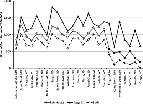
The 18 high-precision rain gauge stations are indicated at left by open symbols, and the seven low-precision stations are indicated at right by solid black symbols. The 3-yr period contains a total of 26,304 hr, so that even the maximum number of hours (1815 hr at Fargo, North Dakota [ND]) corresponds to only 6.9% of the hours in the sampling period.

Figure 2 shows that Stage IV detected precipitation more frequently than rain gauge precipitation at all stations except International Falls, MN. On average, for the high-precision stations, Stage IV detected precipitation 29% more frequently than the rain gauge method. This suggests that the Stage IV method is more sensitive than the rain gauge method, although the Stage IV radar may sometimes be detecting precipitation at cloud level that evaporates before reaching the ground (virga) or precipitation that may be observed within the 4 km × 4 km Stage IV grid area but not at the rain gauge site.

At the low-precision stations, on average, Stage IV detected precipitation about 2.3 times more frequently than low-precision rain gauges. This shows that there were many hours when Stage IV would detect a light precipitation rate of less than 0.10 in/hr, which would accumulate in a rain gauge and be reported at a later hour.

Figure 3 shows a graph of the ratios of the number of hours with measurable precipitation by each method. Open symbols represent high-precision (0.01 in/hr) stations, and black symbols represent low-precision (0.10 in/hr) stations.

Figure 3. Ratios of hours of precipitation in 2006–2008.

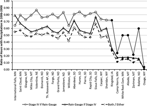
For the high-precision stations, if the rain gauges detected precipitation during a given hour, the probability that Stage IV also detected precipitation during the same hour averaged 78%, and exceeded 70% for all except two stations. If Stage IV detected precipitation during a given hour, the probability that the rain gauges also detected precipitation averaged 60%, and exceeded 52% for all stations. If either method detected precipitation, the probability that both methods detected precipitation simultaneously averaged 51%. This suggests that Stage IV may actually be a more reliable method of detecting precipitation than the rain gauge.

For the low-precision stations, if Stage IV detected precipitation, the probability that the rain gauge also detected precipitation (black triangles) averaged only 18%, and was less than 20% for all stations except one. Since the comparable probability was 60% for high-precision stations, this shows that low-precision rain gauges are not reliable for detecting precipitation during the hour in which it actually falls.

Although the statistical analyses were performed between Stage IV precipitation and rain gauge precipitation from all 25 stations as originally prescribed in the evaluation plan, the TD3240 rain gauge data from the seven low-precision stations have been shown to not be precise enough to be used as a basis of comparison with validated Stage IV precipitation data. Therefore, for the purpose of this paper, only the results of the statistical analyses comparing the Stage IV precipitation with the 18 high-precision rain gauge stations are presented. These are the only stations for which a statistical comparison can determine the validity of Stage IV data, since both methods measure precipitation to an equivalent precision.

Mean bias

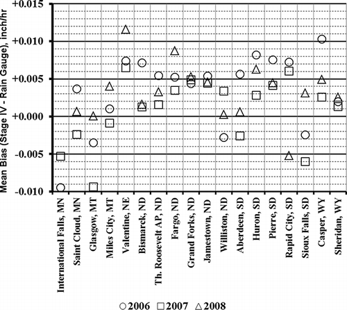
Figure 4 illustrates the mean bias in in/hr, calculated using eq 4, for Stage IV precipitation relative to TD3240 rain gauge precipitation, for each combination of station and year. For these stations, the mean bias is positive for 42 of 53 (79%) combinations of station and year, meaning that Stage IV precipitation tends to be slightly higher than TD3240 rain gauge precipitation. The mean bias is within the precision of measurement (±0.01 in/hr) for 51 of 53 (96%) combinations of station and year.

Figure 4. Mean bias (Stage IV − rain gauge), in/hr.

Mean absolute error

Figure 5 illustrates the mean absolute error in in/hr, calculated using eq 5, for Stage IV precipitation relative to TD3240 rain gauge precipitation, for each combination of station and year.

Figure 5. Mean absolute error (Stage IV − rain gauge), in/hr.

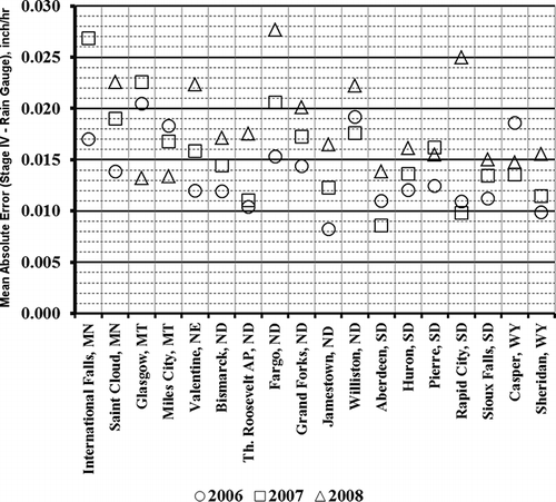
The mean absolute error averaged 0.016 in/hr, and was between 0.01 and 0.02 in/hr for 40 of 53 (75%) combinations of station and year. Since the mean biases (Figure 4) for these stations were mostly between 0.00 and +0.01 in/hr, this indicates that some small negative errors (Stage IV < TD3240 data for some hours) partially canceled out slightly larger positive errors (Stage IV > TD3240 data) to result in a small positive mean bias.

Total annual precipitation

Figure 6 shows a scatter plot of total annual Stage IV precipitation as a function of total annual TD3240 rain gauge precipitation for each station and year.

Figure 6. Total annual Stage IV precipitation as a function of total annual rain gauge precipitation.

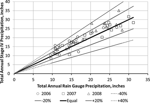
The solid black diagonal line represents points where Stage IV precipitation equals TD3240 rain gauge precipitation. The inner, gray lines represent points where Stage IV precipitation is 20% greater than or less than TD3240 rain gauge precipitation, and the outer, thin dashed lines represent points where Stage IV precipitation is 40% greater than or less than TD3240 rain gauge precipitation, respectively.

Total annual Stage IV precipitation tended to be slightly higher than annual TD3240 rain gauge precipitation, with 32 of 53 (60%) of combinations of station and year between 0% and 20% higher. This shows fairly good agreement between the two methods, and the Stage IV method is slightly more sensitive to precipitation than the rain gauge.

Linear regressions of hourly precipitation rates

Slope and intercept

Figure 7 shows a graph of the intercept b_iy (in in/hr) as a function of the slope m_iy of linear regressions (see eq 6) of Stage IV hourly precipitation as a function of TD3240 rain gauge hourly precipitation rates, for those hours when at least one method recorded precipitation.

Figure 7. Intercept and slope of linear regression of Stage IV precipitation as function of rain gauge precipitation.

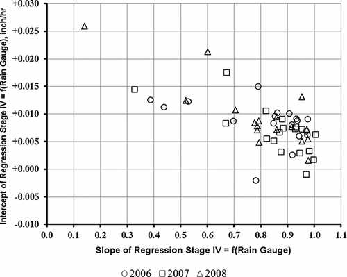
If there was perfect agreement between the methods for all hours, the slope m_iy would be 1.0, and the intercept b_iy would be 0. For the actual data, 51 of 53 (96%) combinations of station and year have positive intercepts and slopes less than 1.0.

For these stations, 31 of 53 (58%) combinations of station and year have intercepts less than 0.01 in/hr (the precision of measurement) and slopes greater than 0.8, which would suggest that Stage IV precipitation rates would be slightly higher at low (or zero) rain gauge precipitation rates, but converge toward near equality at high rain gauge precipitation rates. Another 8 combinations (15%) have slopes and intercepts narrowly outside these ranges. This trend is also observed in scatter plots of hourly Stage IV precipitation as a function of hourly rain gauge precipitation for many of the stations.

Correlation coefficient

Figure 8 illustrates the correlation coefficient r_iy of linear regressions of hourly Stage IV precipitation as a function of hourly rain gauge precipitation, for hours when at least one method detected precipitation. For the high-precision stations, 27 of 53 (51%) combinations of station and year showed correlation coefficients greater than 0.90, indicating an excellent correspondence between hourly Stage IV and hourly rain gauge precipitation. Forty of 53 (75%) combinations showed correlation coefficients greater than 0.80, which can be considered a generally good correspondence between the methods.

Figure 8. Correlation coefficient Stage IV as a function of rain gauge data.

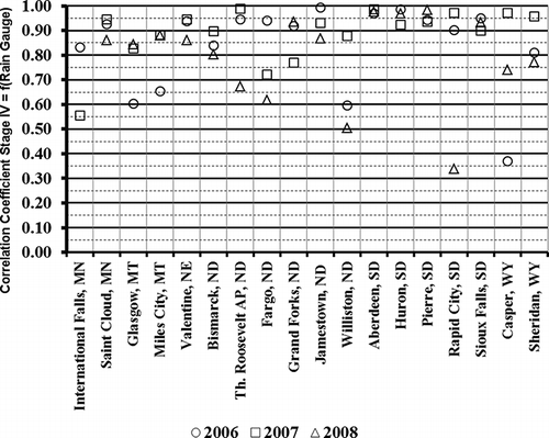
Combining these high correlation coefficients with the small positive intercepts (<0.01 in/hr) and slopes between 0.8 and 1.0 shows that, for 75% of the combinations of station and year, Stage IV hourly precipitation rates show an excellent correlation with rain gauge data at high precipitation rates, and tend to be slightly higher at low (or zero) precipitation rates.

For some stations with lower correlation coefficients (<0.70), a more detailed analysis of scatter plots showed a good-to-excellent correlation for most hours, with a few “outliers” where one method showed a high precipitation rate, and the other method showed zero precipitation. This could be due to a temporarily malfunctioning rain gauge or possibly due to the difference in the Stage IV measurement representing a 4 km × 4 km area versus a specific point for the rain gauge.

Scatter plots of hourly precipitation data

In order to illustrate these trends, five sample scatter plots (Figures 9 through 13) from different stations of hourly Stage IV precipitation as a function of simultaneous rain gauge precipitation measurements in the year 2006 are presented below. The graphs show the simultaneous Stage IV and rain gauge precipitation during a particular hour (which may occur more than once per year), the diagonal black line (y = x) connects points where Stage IV and rain gauge hourly precipitation are equal, and the gray line represents the linear regression of all points not on the origin.

Figure 9. Scatter plot of hourly Stage IV precipitation as a function of hourly rain gauge precipitation: Jamestown, ND, in 2006.

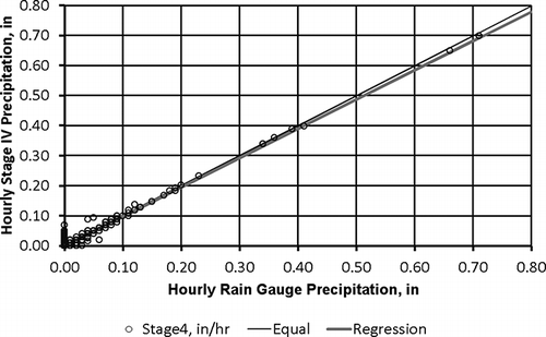
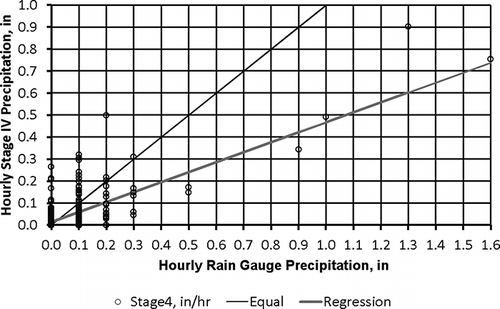
Figure 9 shows the scatter plot for Jamestown, ND, in 2006, whose regression line has a slope of 0.974 and a correlation coefficient of 0.993 (the highest of all stations). Most of the points lie very close to both the diagonal (y = x) line and regression line, although several points along the y-axis indicate hours where Stage IV detected precipitation of 0.07 in/hr or less when the rain gauge did not detect precipitation. It should be noted that this excellent agreement was obtained for a location 121 km from the nearest NEXRAD radar site.

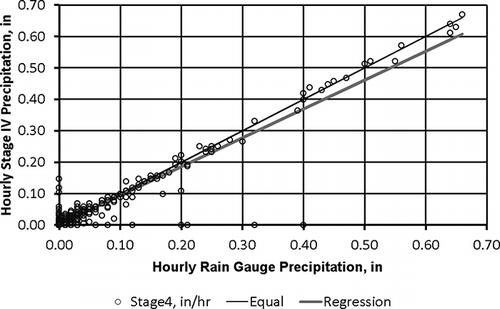
Figure 10 shows the scatter plot for Sioux Falls, South Dakota (SD), in 2006, whose regression line has a slope of 0.949 and a correlation coefficient of 0.917. Most of the points lie very close to the diagonal black (y = x) line for precipitation rates above 0.06 in/hr, showing excellent agreement between the two methods. There are five points where the rain gauge measured more than 0.10 in/hr where Stage IV did not measure precipitation, and three points where Stage IV measured more than 0.10 in/hr and the rain gauge did not measure precipitation. These outliers caused the regression line to lie mainly below the y = x line.

Figure 10. Scatter plot of hourly Stage IV precipitation as a function of hourly rain gauge precipitation: Sioux Falls, SD, in 2006.

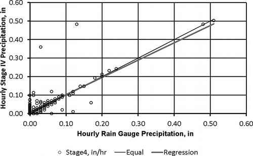
Figure 11 shows the scatter plot for Bismarck, ND, in 2006, whose regression line has a slope of 0.935 and a correlation coefficient of 0.839. There are fewer hours of precipitation greater than 0.10 in/hr than in Sioux Falls, but there is still good agreement between the two methods for most of the hours. However, there are two major outliers where Stage IV detected much more precipitation than the rain gauge, which caused a positive intercept, and the correlation coefficient to be much lower than at Sioux Falls. It is not clear whether these discrepancies are due to errors in the Stage IV method, a temporary failure of the rain gauge during two hours of heavy precipitation, or localized convective precipitation missed by the rain gauge.

Figure 11. Scatter plot of hourly Stage IV precipitation as a function of hourly rain gauge precipitation: Bismark, ND, in 2006.

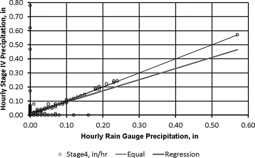
Figure 12 shows the scatter plot for Casper, Wyoming (WY), in 2006, whose regression line has a slope of 0.790 and a correlation coefficient of 0.369, which is the lowest correlation coefficient for all high-precision stations. Despite the low correlation coefficient, most of the points are close to the diagonal (y = x) line, indicating good agreement between the two methods for most hours. The regression line and correlation coefficient are skewed by 3 hr where Stage IV recorded more than 0.46 in/hr, but the rain gauge recorded zero precipitation. It is not clear whether this is due to a Stage IV error, a failure of the rain gauge during these 3 hr, or localized convective precipitation missed by the rain gauge.

Figure 12. Scatter plot of hourly Stage IV precipitation as a function of hourly rain gauge precipitation: Casper, WY, in 2006.

As an example of a low-precision rain gauge, Figure 13 shows the scatter plot for Ringsted IA in 2006, whose regression line has a slope of 0.453 and a correlation coefficient of 0.748 (the highest of all low-precision TD3240 stations). When the rain gauge detects 0.1 in/hr, the Stage IV measurements tend to “straddle” this value, but the Stage IV measurements tend to be much lower than the rain gauge measurements at higher precipitation rates. This is the opposite of the trend for high-precision stations, where the two methods show the best agreement at high precipitation rates. This indicates that the low-precision rain gauges do not provide reliable data, and should not be used as a basis of comparison with Stage IV precipitation rates. The low-precision rain gauges seem to exaggerate precipitation rates during periods of heavy precipitation.

Figure 13. Scatter plot of hourly Stage IV precipitation as a function of hourly rain gauge precipitation: Ringsted, IA, in 2006.

Effect of type of rain gauge

The 18 high-precision rain gauges in this study were of three different types:

•	tipping bucket (TB-unheated)
•	Automated heated tipping bucket (AHTB)
•	All-weather precipitation accumulation gauge (AWPAG)

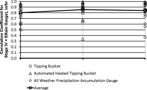
In order to determine whether the type of rain gauge with which Stage IV precipitation data are compared has any effect on the degree of correlation or agreement, the mean bias (Figure 14), mean absolute error (Figure 15), and correlation coefficient (Figure 16) for each combination of high-precision gauge and year were plotted as a function of gauge type. The black line on each graph connects the average values for all combinations of years and stations of a given type. These statistics are only calculated for hours when at least one method records measurable precipitation and dry hours are excluded from these analyses.

Figure 14. Mean bias (Stage IV − rain gauge) for high-precision stations as a function of rain gauge type.

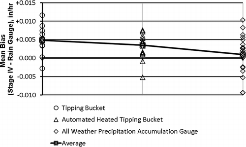
Figure 15. Mean absolute error (Stage IV − rain gauge) for high-precision stations as a function of rain gauge type.

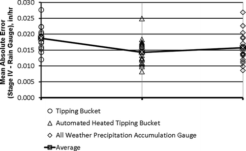
Figure 16. Correlation coefficient, Stage IV, as a function of rain gauge data for high-precision stations categorized by rain gauge type.

The mean bias, or average amount by which Stage IV precipitation exceeds the rain gauge precipitation, tends to be highest for tipping bucket gauges (+0.0049 in/hr on average), slightly lower for AHTB gauges (+0.0035 in/hr on average), and lowest for AWPAGs (+0.0010 in/hr on average). There is considerable overlap in the mean biases between the different gauge types, and the AWPAG gauges have the best balance between positive and negative mean biases. All except two of the mean biases are within the precision of the methods (0.01 in/hr).

The mean absolute error tends to be lowest for AHTB gauges (0.0143 in/hr on average), with AWPAGs slightly higher at (0.0157 in/hr on average), and highest for tipping bucket gauges (0.0187 in/hr on average). There is considerable overlap between the values of mean absolute error between the different gauge types.

The correlation coefficient tends to be highest for AHTB gauges (0.857 on average), with AWPAGs slightly lower at 0.841 on average, and lowest for tipping bucket gauges (0.802 on average). The correlation coefficient is consistently higher for AHTBs, with only three values below 0.800, as compared with five values below 0.800 for each of the other two gauge types.

In terms of overall agreement with Stage IV data, the AHTBs and AWPAGs seem to be of about equal quality (with a slight advantage for AWPAG because of the lower absolute bias), whereas the unheated tipping bucket gauges show more deviation from Stage IV precipitation by all methods. The trends concerning the averages should be interpreted with caution, because values for all three statistics overlap between the gauge types.

Effect of distance from NEXRAD radar site

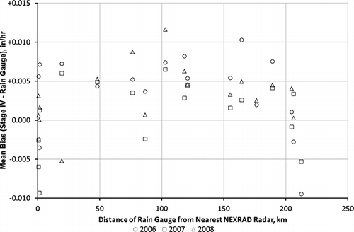
In order to test whether the accuracy of Stage IV precipitation measurements is affected by the distance of a precipitation station from the nearest radar NEXRAD radar site, graphs were prepared of mean bias, mean absolute error, and correlation coefficient for the high-precision rain gauge stations as functions of distance from the nearest NEXRAD radar site (from Table 2).

Of the 18 high-precision stations in this study, 4 are within 2 km of a NEXRAD radar site; 4 additional stations are less than 100 km from a radar site; another 7 are 100–200 km from the nearest radar site; and 3 are more than 200 km from the nearest radar site.

Figure 17 shows the mean bias (Stage IV − rain gauge) for all combinations of high-precision station and year as a function of distance from the nearest NEXRAD radar site. For the four stations within 2 km of a radar site, mean bias was nearly evenly distributed around zero, as was true for the three stations more than 200 km from the nearest radar site. For stations between 19 and 200 km from the nearest radar site, mean biases tended to be positive (31 of 33 combinations), generally centered around +0.005 in/hr. A positive mean bias indicates that hourly Stage IV precipitation tends to be higher than rain gauge precipitation for the same hour.

Figure 17. Mean bias of Stage IV − rain gauge precipitation (in/hr) for high-precision stations as a function of distance from NEXRAD radar.

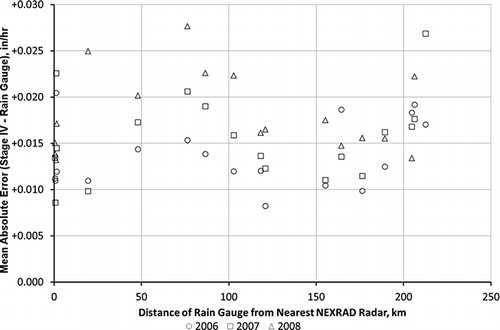
Figure 18 shows the mean absolute error (Stage IV − rain gauge) for all combinations of high-precision station and year as a function of distance from the nearest NEXRAD radar site. For the four stations within 2 km of a radar site, the mean absolute errors were clustered between 0.011 and 0.015 in/hr. Similar values (0.010–0.018 in/hr) were obtained for sites 100–200 km from the nearest NEXRAD site. Mean absolute errors were slightly higher for stations between 19 and 100 km, and more than 200 km from the nearest NEXRAD radar site. It is not clear whether or not these trends are significant, due to the small number of stations, and variations in rain gauge type.

Figure 18. Mean absolute error of Stage IV − rain gauge precipitation (in/hr) for high-precision stations as a function of distance from NEXRAD radar.

Figure 19 shows the correlation coefficient for all combinations of high-precision station and year as a function of distance from the nearest NEXRAD radar site. For the stations within 2 km of a radar site, 11 of 12 correlation coefficients are above 0.800. For the stations more than 200 km from the nearest radar site, all correlation coefficients were less than 0.900. For distances between 19 and 200 km, the correlation coefficients are irregular, with 21 of 33 values above 0.900, but 8 of 33 values below 0.800.

Figure 19. Correlation coefficient of Stage IV as a function of rain gauge for high-precision stations shown in relation to distance from NEXRAD radar.

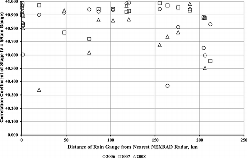
Overall, the stations within 2 km of a NEXRAD radar site show the best fit with TD3240 rain gauge data (mean bias near zero, low mean absolute error, and high correlation coefficient). Stations more than 200 km from the nearest NEXRAD radar site fit less well with TD3240 rain gauge data (slightly higher mean absolute errors and lower correlation coefficients). At intermediate distances, the trends are irregular, with a slight tendency for Stage IV precipitation to be higher than rain gauge precipitation (positive mean bias), and other statistics similar to those of the stations very close to the radar sites.

These results need to be interpreted with caution, due to the relatively small number of stations studied, and the variation in the type of rain gauge with which Stage IV data are compared.

Quarterly statistical analysis in 2006

In order to determine whether there may be a seasonal dependence of the correlation between Stage IV and rain gauge precipitation, statistical analyses were performed for the high-precision stations for 3-month periods in 2006 for winter (January–March); spring (April–June); summer (July–September); and autumn (October–December). For the mean bias and mean absolute error statistics, the denominator is the total number of hours per quarter where either the rain gauge or Stage IV recorded measurable precipitation, whereas dry hours (where neither method recorded precipitation) are not included in these statistics.

Number of hours of precipitation

Figure 20 shows a scatter plot of the number of hours where Stage IV detected precipitation during each quarter, as a function of the number of hours where the rain gauge detected precipitation.

Figure 20. Quarterly hours of nonzero precipitation by Stage IV and rain gauge in 2006 (high-precision stations).

Figure 20 shows that precipitation according to both methods is more frequent in spring and summer than in autumn or winter. Stage IV precipitation was more frequent than the rain gauge precipitation for 60 of 72 (83%) combinations of station and season, with 5 of the 12 exceptions in autumn.

The ratio of hours of Stage IV precipitation to hours of rain gauge precipitation tends to be much higher in winter than in other seasons. This is probably due to the difficulty of detecting blowing snow in a rain gauge, whereas the Stage IV radar is sensitive to both rain and frozen precipitation. In other seasons, when most precipitation is liquid, Stage IV still detects precipitation more frequently than the rain gauges, but the frequency ratio is much closer to unity.

Quarterly mean bias

The quarterly mean bias (Stage IV − rain gauge) followed the same trends as the annual mean bias data. A majority of the stations had positive mean biases between 0 and +0.01 in/hr in all seasons, meaning that Stage IV showed slightly higher precipitation on average, but within the precision of the measurement. The average mean bias for all stations for a given season varied between +0.0016 in/hr (spring) and +0.0047 in/hr (winter), but this seasonal variation is not considered significant.

Quarterly mean absolute error

The quarterly mean absolute error between Stage IV and rain gauge hourly precipitation data followed the same trends as the annual mean absolute error data, with 42 of 72 (58%) of combinations of station and season having a mean absolute error between 0.01 and 0.02 in/hr, and 63 of 72 (88%) combinations with mean absolute errors less than 0.02 in/hr. The average mean absolute error for stations for a given season varied between 0.0125 in/hr (autumn) and 0.0148 in/hr (spring), but this seasonal variation is not considered significant.

Total quarterly precipitation

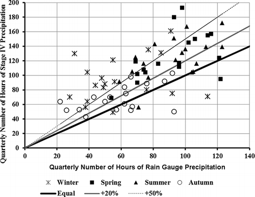
Figure 21 shows a scatter plot of the total quarterly Stage IV precipitation during each quarter, as a function of the total quarterly rain gauge precipitation measurement.

Figure 21. Quarterly Stage IV precipitation as a function of quarterly rain gauge precipitation in 2006.

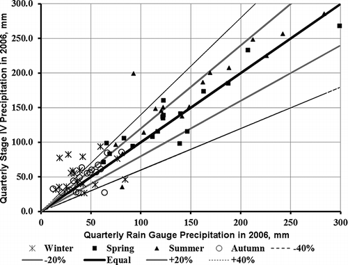
Figure 21 shows that total quarterly precipitation according to both methods is much higher in spring and summer than in autumn or winter.

Stage IV precipitation was higher than rain gauge precipitation for at least 12 of 18 stations in all seasons; however, the difference was less than 20% for a majority of stations in summer and autumn. Stage IV precipitation tended to be much higher than the rain gauge precipitation in winter, with the difference greater than 40% for half of the stations. This is probably due to the difficulty of measuring blowing snow in a rain gauge, whereas the Stage IV radar can detect both rain and frozen precipitation.

Spatial resolution of Stage IV and rain gauge data

The Stage IV precipitation data set is being considered for use in atmospheric dispersion models primarily due to its much finer spatial resolution (4 km × 4 km squares) than ground-based rain gauges, which may be widely separated in sparsely populated areas such as the north central United States. This section shows an example of the difference in spatial resolution of precipitation data between the Stage IV and rain gauge data, for the total precipitation in the year 2007.

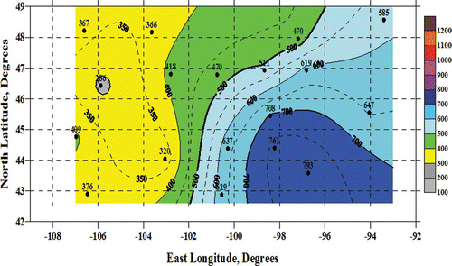
Figure 22 shows an isopleth diagram of the geographical distribution of the total annual precipitation (in millimeters) during the year 2007 as measured by the 18 high-precision rain gauges. The black circles on Figure 22 show the geographical location of each station, and the number above each circle shows the total annual precipitation at the station. The isopleth lines were interpolated using the Kriging technique.

Figure 22. Geographical distribution of total annual precipitation (mm) in 2007 (18 high-precision rain gauge stations).

Figure 23 shows a comparable diagram of the geographical distribution of the total annual precipitation (in millimeters) during the year 2007 as measured by the Stage IV method at the 25 (high-precision and low-precision) rain gauge locations used for statistical comparison in this paper. The same shading is used for each isopleth interval in Figures 22 through 24.

Figure 23. Geographical distribution of total annual precipitation (mm) in 2007 Stage IV, at 25 selected rain gauge stations.

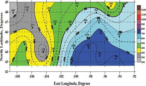
The geographical distributions of total annual precipitation by the two methods are similar over most of the region, showing a good agreement of Stage IV precipitation with the high-precision rain gauges.

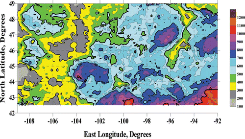
In the region between 42.5°N and 49°N latitude, and 92°W and 109°W longitude, there are 52,011 Stage IV grid points at a 4 km × 4 km spatial resolution. Figure 24 shows an isopleth diagram of the geographical distribution of total Stage IV precipitation in 2007 at all these grid points.

Figure 24. Geographical distribution of total annual precipitation (mm) in 2007 Stage IV: 52,011 grid points, 4 km × 4 km spatial resolution.

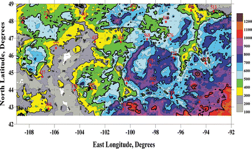
Figure 24 clearly shows that the 4 km × 4 km resolution of Stage IV data can resolve local precipitation events, and spatial variations in precipitation, that can be often missed by widely spaced rain gauges. There are significant differences in the precipitation pattern shown in Figure 24 compared with patterns in Figures 22 and 23. For example, consider the general area of low precipitation (<400 mm) west of 104°W longitude in Figures 22 and 23. In Figure 24, it is replaced by areas of extremely low precipitation (<200 mm), precipitation above 500 mm/yr, and a localized area of high precipitation (>600 mm) north of 48°N between 99°W and 102°W, which were not evident in Figures 22 and 23. It is possible that the differences may be real or may be attributed to Stage IV data artifacts, which are not considered in this paper. Further analysis of all available rain gauge data for these areas would be necessary to make a definitive determination.

Comparison of Stage IV geographical distribution between years

Figure 25 shows an isopleth diagram of the geographical distribution of total Stage IV precipitation in 2006 at 4 km × 4 km resolution, using the same contour interval (100 mm) and shading as in Figures 22 through 24. Figure 26 shows a similar isopleths diagram for geographical distribution of Stage IV precipitation in 2008.

Figure 25. Geographical distribution of total annual precipitation (mm) in 2006 Stage IV: 52,011 grid points, 4 km × 4 km spatial resolution.

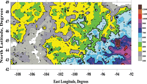
Figure 26. Geographical distribution of total annual precipitation (mm) in 2008 Stage IV: 52,011 grid points, 4 km × 4 km spatial resolution.

Although there are some significant differences from year to year (2006 was drier than 2007 throughout the region studied; 2008 was wetter than 2007 in western parts of the region), there are many similarities in the patterns of geographical distribution of total annual precipitation from year to year.

Summary of Conclusions

In order to more accurately model the long-range wet deposition of particulate matter and water-soluble pollutants, long-range dispersion models such as CALPUFF require input of hourly precipitation data over large geographical areas and long modeling periods.

The Stage IV precipitation measurement database, which contains hourly precipitation data for a grid of 4 km × 4 km squares covering the continental United States, would enable the input of precipitation data over a much finer spatial resolution than widely spaced ground-based precipitation measurement stations, particularly in sparsely populated areas such as the north central United States.

The purpose of this statistical study was to validate the reliability of radar-based Stage IV hourly precipitation rates by comparing these with simultaneous precipitation rates measured at 25 ground-based rain gauge stations at the same locations over the 3-yr period from 2006 through 2008.

The 25 precipitation stations used for this statistical study included 18 “high-precision” stations where hourly precipitation was measured to a precision of 0.01 in, and seven “low-precision” stations where hourly precipitation was measured to a precision of 0.10 in.

By every statistical criterion evaluated in this study, the hourly precipitation data from the seven low-precision TD3240 stations were much less reliable than those from the 18 high-precision TD3240 stations. The input to a dispersion model of low-precision rain gauge data, which neglect some hours of light precipitation and regroup the rain into a single hour, would introduce significant errors in the wet deposition of pollutants. This is because small droplet sizes during light precipitation have a relatively high surface area for absorption and may be reported during hours with different weather than actually occurred. Therefore, low-precision rain gauge precipitation data do not seem appropriate for use in dispersion models, and should not be used as a basis for determining the validity of Stage IV precipitation data.

Due to the limitations of low-precision rain gauge data, the validity of the Stage IV hourly precipitation data is based only on the comparison of Stage IV data with simultaneous rain gauge data from the 18 high-precision stations, where both measurement methods have a precision of 0.01 in/hr.

The overall statistical analyses presented in this paper show that Stage IV hourly precipitation is well correlated with rain gauge hourly precipitation (from high-precision stations) at high precipitation rates. Analyses of scatter plots (not shown here) tend to show slightly higher and more frequent precipitation than rain gauges at low precipitation rates, with the mean bias within the precision of measurement in most cases.

Stage IV and rain gauge measurement data are well correlated at high precipitation rates, when wet deposition rates of pollutants are highest, thus use of Stage IV precipitation rates in dispersion models would accurately model the wet deposition rates during heavy precipitation.

If Stage IV detects light precipitation during an hour when the rain gauge does not, it could be due to the Stage IV radar detecting “virga”—cloud-level precipitation that evaporates before reaching the ground. It is also possible that light precipitation detected by Stage IV may reach the ground, but some of the precipitation evaporates during the hour before 0.01 in has accumulated to “trip” a rain gauge and record the precipitation or that the Stage IV data detected light precipitation within the 4 km × 4 km grid cell that was not detected or observed at the rain gauge site.

In the case of “virga” that does not reach the ground, any absorbed water-soluble pollutants would be re-released into the atmosphere, and using a zero precipitation rate from the rain gauge data would accurately model the (lack of) wet deposition.

In the case of light precipitation that reaches the ground but does not trip a rain gauge, water-soluble pollutants would reach the ground, and the wet deposition would be more accurately modeled using the Stage IV precipitation data.

Based on the analyses performed, it can be concluded that Stage IV and high-precision rain gauge precipitation data are equally suitable for use in dispersion models, based on their ability to accurately predict wet deposition at a given location.

However, since Stage IV precipitation data are available at a finer spatial resolution (4 km) than data from high-precision rain gauges, it would be more accurate to use gridded Stage IV precipitation data appropriate for a specific modeling domain in a gridded dispersion model for a long-range simulation, than to rely on precipitation data interpolated between widely scattered rain gauges.

References

- Habib , E. , Larson , B.F. and Graschel , J. 2009 . Validation of NEXRAD multisensory precipitation estimates using an experimental dense rain gauge network in south Louisiana . J. Hydrol , 373 : 463 – 478 . doi: 10.1016/j.jhydrol.2009.05.010
- National Centers for Environmental Prediction, 2012. National Stage IV QPE Mosaic at NCEP http://www.emc.ncep.noaa.gov/mmb/ylin/pcpanl/stage4/ (accessed February, 1, 2013) (http://www.emc.ncep.noaa.gov/mmb/ylin/pcpanl/stage4/ (accessed February, 1, 2013))
- National Climatic Data Center. 2013. Climate data online http://www.ncdc.noaa.gov/cdo-web/ (accessed February 1, 2013) (http://www.ncdc.noaa.gov/cdo-web/ (accessed February 1, 2013))
- National Weather Service, 2005. NWS ASOS Program http://www.nws.noaa.gov/asos/index.html (accessed February, 1, 2013) (http://www.nws.noaa.gov/asos/index.html (accessed February, 1, 2013))
- National Weather Service, 2012. Hydrometeorological Automated Data System http://www.nws.noaa.gov/oh/hads (accessed February, 1, 2013) (http://www.nws.noaa.gov/oh/hads (accessed February, 1, 2013))
- Over , T.M. , Murphy , E.A. , Ortel , T.W. and Ishii , A.L. 2007 . “ Comparisons between NEXRAD radar and tipping bucket gage rainfall data: A case study for DuPage County, Illinois ” . In Proceedings, ASCE-EWRI World Environmental and Water Resources Congress In 1–14. Tampa, FL: American Society of Civil Engineers.
- Sexton , A.M. , Sadeghi , A.M. , Zhang , X. , Srinivasan , R. and Shirmohammadi , A. 2010 . Using NEXRAD and rain gauge precipitation data for hydrologic calibration of SWAT in a northeastern watershed . Trans. Am. Soc. Agric. Biol. Eng , 53 : 1501 – 1510 .
- Wang , J. and Wolff , D.B. 2009 . Evaluation of TRMM ground-validation radar-rain errors using rain gauge measurements . Environ. J. Appl. Meteorol , 49 : 310 – 324 . doi: 10.1175/2009JAMC2264.1
- Young , C.B. , Bradley , A.A. , Krajewski , W.F. and Kruger , A. 2000 . Evaluating NEXRAD multisensor precipitation estimates for operational hydrologic forecasting . J. Hydrometeorol , 1 : 241 – 254 . doi: 10.1175/1525-7541(2000)0012.0.CO;2
- Zhang , X. and Srinivasan , R. 2010 . GIS-based spatial precipitation estimation using next generation radar and rain gauge data . Environ. Model. Softw , doi: 10.1016/j.envsoft.2010.05.012