Comparison of variability in dioxin and furan data acquired using single train and simultaneous multiple train stack sampling methods

Abstract

The variance of polychlorinated dibenzo-p-dioxin (PCDD; dioxin) and polychlorinated dibenzofuran (PCDF; furan) data obtained from single- and simultaneous multiple train methods was compared. Single train triplicate data were used from 4 stack tests obtained from a long dry kiln cement plant and 18 stack tests from a municipal solid waste (MSW) incinerator. Data from the American Society of Mechanical Engineers (ASME) report Reference Method Accuracy and Precision (ReMAP) (Lanier and Hendrix, 2001) were used for the simultaneous multiple samples, which accounted for 27 data points. Nineteen data points were acquired from an ASME research facility, 5 from a MSW incinerator unrelated to the single train MSW incinerator, and 3 from a lightweight aggregate kiln (LWAK). The ReMAP procedure was used to determine the relationship between the standard deviation and the concentration of the single train and simultaneous multiple train data. Results indicated that there was benefit from the use of simultaneous multiple train sampling for concentrations above 129 pg toxic equivalency (TEQ)/m³. There was no indication of benefit from the use of simultaneous multiple train sampling at concentrations below 129 pg TEQ/m³.

Implications:

Precision of stack sampling data can be the difference between meeting and failing compliance limits. Generally, three dioxin/furan samples are acquired when stack sampling to meet compliance regulations. A reliable estimation of the data’s true concentration is not possible with this small amount of data. Increasing the precision decreases the chance that the acquired concentration deviates greatly from the true concentration. Facilities that use the appropriate stack sampling method will benefit by either improved data precision or minimal stack sampling expenses. The observations made suggest that facilities that are expected to have dioxin/furan concentrations above 129 pg TEQ/m³ would increase the precision of samples by using simultaneous multiple train sampling.

Introduction

The chemical characteristics of a waste gas stream that is emitted into the atmosphere from an industrial facility are typically determined through gas sampling in the exhaust stream (stack sampling). Stack sampling is used to determine compliance to regulations, to compare concentrations of emissions between facilities, to create emissions inventories, and to determine changes in concentrations that have occurred due to process alterations at a facility (U.S. Environmental Protection Agency [EPA], n.d.-a). In the USA, failure to meet compliance regulations can lead to charges, substantial fines, and retesting. Thus, significant expenses can be the result of a failed compliance test. There is inherent uncertainty associated with the results acquired from stack sampling. Increasing the precision of sampling methods may be the difference between meeting and failing compliance conditions. Simultaneous multiple train stack sampling is a method that can decrease the variability of stack sampling at certain sample concentrations. This paper compared the variability of single train and simultaneous multiple train sampling methods where the organic compounds polychlorinated dibenzo-p-dioxins (PCDD; dioxins)/polychlorinated dibenzofurans (PCDF; furans) are considered to ascertain when the added cost of simultaneous multiple train sampling may be warranted.

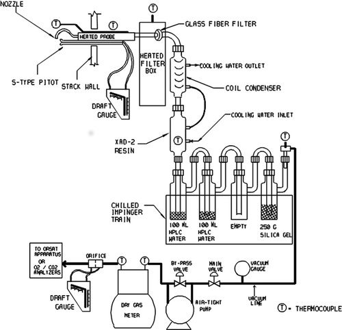
Samples of stack gas were extracted following EPA Method 23 (EPA, n.d.-b). Samples were acquired isokinetically from an apparatus called a sampling train. As seen in Figure 1, the train consisted of a sampling probe, a heated line, a heated filter, a module filled with a polymeric absorbent (Amberlite XAD-2 Polymeric Adsorbent, Supelco, Bellefonte, PA, USA), and a series of interconnected glass vessels, called impingers, immersed in an ice bath. The probe assembly typically consists of a 1-inch-diameter stainless steel tube, a heated glass probe liner, an S-type Pitot probe attached with 3/8-inch-diameter tubing, and a 1/4-inch-diameter thermocouple. The Pitot tube and thermocouple are used to determine the velocity and temperature, respectively, at the sampling location. These provide information to adjust the sampling rate to isokinetic conditions. Isokinetic sampling conditions exist when the mean velocity inside the probe entrance equals the local stack velocity. If the probe and stack were to have different velocities, there would be resistance or suction occurring at the probe inlet, which prevents the collection of an accurate representation of the flue gas, especially for flue gasses containing particulate matter (Lanier and Hendrix, 2001).

Figure 1. Diagram of EPA Method 23.

Typically regulations require that three separate samples be collected using the sampling train discussed in the previous paragraph. This equipment is operated by two technicians. The sampling train probe is traversed across equal-area segments of the stack, stopping at each location for a uniform time. The total sampling time is dictated by analytical capability and the expected analyte concentrations, and in most cases exceeds 3 hr in duration. For circular stacks, a cross-sectional plane is separated into multiple equal-area segments as a function of the distance from the center of the stack. A minimum of two traverses are performed, separated by 90°, with the sampling occurring at the center of each equal-area segment. For square or rectangular stacks, a cross-section of the stack is separated into a grid of equal areas. Sampling is performed on the centroid of each of these sections. The minimum number of sampling points is specified by the method and is a function of the size of the stack (EPA, n.d.-a; Ontario Ministry of the Environment, 2009). Since each sample is obtained over a different time interval, the variability observed is the result of a series of three tests and should be the result of process variability from the facility and variability from the sampling methods (Moffat, 1988).

Simultaneous train sampling uses multiple sampling systems to acquire samples concurrently. The probes can be inserted through the same port with the sampling nozzles located a short distance from one another, or they can be inserted through separate ports with the traverses switched to cover each equal-area segment. Inserting the probes through the same port is a more challenging implementation due to the added bulk and mass from combining two sampling trains. Regardless of the configuration chosen, extra field technicians during sampling and extra laboratory analytical work would be required. By acquiring multiple samples simultaneously, the variability in the sampling methods can be isolated because it can be assumed that the process related variations occurring during sampling are captured equally by each train.

The report Reference Method Accuracy and Precision (ReMAP) used simultaneous sampling data to determine the precision of the EPA sampling methods, and established the relationship between the concentration and standard deviation of the test results. For simultaneous multiple train sampling, it is assumed that there are minimal differences in the flue gas flow velocity and composition at the probe inlets. The simultaneous data therefore should ideally be identical. Variability in the measured concentration from a single simultaneous multiple train stack test should be the result of random error from the stack testing method (Lanier and Hendrix, 2001). ReMAP considered 22 simultaneous PCDD/PCDF sampling results from two facilities, and in a subsequent update, added 5 simultaneous results from a third facility. These data were used to provide an estimate of the precision of EPA Method 23 at various analyte concentration levels. Nineteen stack samples were obtained from a project undertaken for the American Society of Mechanical Engineers (ASME) at a municipal solid waste (MSW) incineration research facility, five from a second MSW, and three from a lightweight aggregate kiln (LWAK). The ASME research data were obtained from the midpoint in the air pollution control system, after powdered activated carbon (PAC) and acid gas reagent addition and the electrostatic precipitator (ESP), but before final polishing and therefore did not represent the stack emission levels; however, due to the limited availability of simultaneous PCDD/PCDF data, the ASME research data are useful in extending the data coverage. The purpose of that study was to establish factors that influence the level of control of the air pollution control (APC) system. Using fractional factorial experimental test plans to examine the effect of varying incinerator operating temperature, oxygen levels, and the feed rate of both lime and PAC injected in the ductwork, a range of emission concentrations was generated. These data were then used to ascertain factors that would limit emissions. The sampling was conducted in a square duct, with dimensions of 0.8 m by 0.8 m. There were four ports used at the sampling location. Two probes were physically linked together a short distance from each other (approximately 6–8 inches) and inserted into the ports to simultaneously acquire the samples over a period of 2.4 hr. (ASME Research Committee on Industrial and Municipal Waste, 1997). The second MSW incinerator and LWAK data were obtained from a location in the stack that was 8 diameters downstream and 2 diameters upstream from a flow disturbance. The MSW incinerator stack is a rectangular concrete structure with two flue liners of internal 1.33 m diameter. There are two sampling ports on each flue liner, located 90° from one another. Three stack tests were conducted on each flue liner, with one probe in each port. Sampling was conducted over a period of 4 hr. There was an issue with one test pair, as one train was determined to be invalid by the samplers, resulting in 5 data points. The LWAK sampling was conducted over a period of 3–6 hr on a stack with a large diameter (>1 m) and high flow rate.

The single train data consisted of 4 stack samples obtained from a long dry kiln cement plant and 18 stack samples from an MSW incinerator. Each sample consisted of 3 data points obtained separately on a daily basis. The long dry kiln stack had a diameter of 3.2 m and four sampling ports located at 90° from each other. Sampling was conducted for 120–160 min in 2006, and for 3 hr in 2010 and 2012. Two tests were conducted in 2010, each with different operating conditions. One test was a baseline test, the fuel was a mixture of coal and petroleum coke (petcoke). The second test was conducted during a biomass fuel demonstration project, 90% of the fuel consisted of a mixture of coal and petcoke, 10% was a mixture of biomass fuels: millet, sorghum, hemp, switchgrass, maize, and oat hulls. The tests in 2006 and 2012 were baseline tests. The MSW incinerator stack had a diameter of 2.2 m, with sampling ports located at 90° from one another. Sampling was over a period of 4 hr. Twelve MSW incinerator stack samples were collected from a facility with an APC system that incorporated a wet spray humidifier, lime and PAC injection, fabric filter system, and catalytic destruction of organics in a selective catalytic reduction (SCR) unit that also controls nitrogen oxide (NO_x) emissions. Six MSW incinerator stack samples were from the MSW incinerator stack in the years before the PAC and SCR system were introduced.

Both the cement kiln and the MSW incinerator have tightly controlled operating windows. The cement kiln operators maintain conditions to ensure that the clinker being produced meets the desired quality profile. The MSW incinerator must meet operating requirements reflected by the continuous emissions monitor (CEM) equipment installed at the facility. In both facilities, testing was conducted at typical operating inputs near the maximum design operating capacity. Although the source of the raw material input to the cement kiln can change, this is expected to have little impact on the organic emissions from the facility given the combustion conditions. The MSW incinerator facility has five furnace/boiler units feeding a single APC system. The furnace/boiler units require periodic maintenance, but testing is conducted with the units at various stages of their maintenance cycles, so the emissions represent a blending of any variations that such conditions might produce. The nature of the MSW fed to the incinerators has changed over the period represented by the data considered in this paper, as the community emphasis on recycling and changes in packaging materials have resulted in an increase in plastic and a reduction in metal and paper concentrations. The implementation of the robust APC system produced the biggest change in the emissions at the facility, and, as the data illustrate, there is very little change in emissions year over year. As discussed later in the paper, all the results were analyzed to determine if there was any abhorrent data that might indicate significant variations in the emissions. There were none.

Certain processes have the ability to limit PCDD/PCDF emissions. Cement production requires high temperatures (>1400 °C) and long residence times in the kiln to produce clinker (an intermediate product in the manufacturing of cement). The high temperature and long residence time limits the production of dioxins/furans (Karstensen, 2008). The type of APC system at the MSW facility consisting of PAC addition and catalytic destruction of organics has a removal efficiency of dioxins/furans that can be greater than 90% effective (Chang et al., 2007; Fujii et al., 1994). Thus, the cement kiln and control MSW incinerator emissions should decrease the significance of daily process variability.

PCDD/PCDF data are presented in the mass concentration units pg toxic equivalency (TEQ)/m³. PCDD/PCDF consists of 75 PCDD congeners (related compounds) and 135 PCDF congeners, each with varying levels of toxicity. The toxic equivalency is a number that represents the concentration of dioxins/furans in terms of the most toxic congener, 2,3,7,8-tetrachlorodibenzo-p-dioxin (TCDD). The initial concentration of each congener, in units of pg/m³, was multiplied by its respective toxic equivalence factor (TEF) as determined by International Toxic Equivalents (I-TEQ) (North Atlantic Treaty Organization Committee on the Challenges of Modern Society, 1988), resulting in units of pg TEQ/m³. Nondetectable levels of congeners can be found in laboratory results. These are reported as nondetectable (ND), with the estimated detection level (EDL) and reportable detection level (RDL) being listed for each congener. According to the EPA (EPA, n.d.-c), the sample-specific EDL is a laboratory estimate of the concentration of a given analyte that would produce a signal with a peak height of at least 2.5 times (2.5×) the background noise signal level. Such an estimate is specific to a particular analysis of the sample and is affected by sample size, dilution, etc. The RDL is typically 10× the EDL. If ND levels are reported, there are generally two approaches to calculating the toxic equivalence of the sample, either considering the congener to be not present, or substituting the EDL for that congener and sample in the calculation. Such substitution is required in Ontario as explained in the Ministry of Environment (MoE) Guidline A-8 (Ontario Ministry of the Environment, 2004) and data are reported in that manner to the province. However, with a high proportion of ND values in the data from both the MSW incinerator with the robust APC system and the cement kiln, concerns existed about the potential influence these substitutions might have on the data variability. Helsel (Helsel, 2010) suggests that the substitution approach creates a situation where the less precise data can have a large effect on the result, particularly if the EDL is high, and this can lead to erroneous results when hypothesis testing is performed. He cites the work of several authors showing the inadequacy of the substitution process and recommends the use of the Kaplan-Meier (KM) procedure that is frequently used in survival analysis for computing the mean of right-hand censored data. Essentially the procedure generates the mean of the congener values times their respective TEFs. The mean of the group can be multiplied by 17, the number of congeners considered in the TEQ calculation to provide a reliable method of predicting the mean I-TEQ value for the test and upper confidence limit of the mean. Helsel provides a spreadsheet (Helsel, n.d.) that was used for this study. The resulting mean is based upon parametric procedures that do not require transformations or assumptions about the specific distributional shape of the data. The emission levels encountered at the facilities included in the ReMAP report were generally of sufficient magnitude that ND values were not encountered and no attempt was made to revise the ReMAP data using this approach.

The corrected congener values were summed to determine the overall concentration of the dioxins/furans.

Oxygen correction is a method that is used when comparing concentrations of analytes on a standard basis. Oxygen concentration varies depending on the stack flow rate of air and combustion processes. Normalizing the analyte concentration to a standard basis allows better comparison with other data and to regulatory criteria. For dioxin/furan emissions, regulatory guidelines and limits are based on correction to a stack gas oxygen level of 7% in the USA and commonly 11% in Europe and Canada. Therefore, differences in the flow rate of the air do not affect the concentration of pollutants, allowing data from separate facilities to be compared equally. Oxygen corrections were excluded from the ReMAP analysis to prevent the introduction of uncertainty related to the precision of the oxygen measurement (Lanier and Hendrix, 2001). The oxygen data were therefore unavailable for that data, and oxygen correction was not undertaken for this study.

Due to the additional fixed sources of error in single train sampling procedures, the hypothesis explored in this paper is that the variability of data acquired from stack tests using a single train is greater than the variability of data acquired from simultaneous multiple train sampling methods.

This paper explains the procedure used to determine the relationship between concentration and standard deviation of dioxins/furans. The relationships both including and excluding outliers are plotted and the single and simultaneous multiple train plots are superimposed on one another. The standard deviation’s 95% confidence limits are used to determine the significance between the standard deviation of the single and simultaneous multiple train data. A discussion of the results, conclusions, and recommendations are provided.

Methods

The procedure followed for the study was based upon the premise that the precision of manual stack sampling methods varies as a function of the concentration. The analysis was started by averaging each set of data (triplicate results from single train sampling and paired results acquired from simultaneous multiple train sampling). The standard deviation of these data sets was then determined. Due to the limited number of samples, a small sample bias correction factor was introduced to allow a better estimate of the true standard deviation. Building upon the ReMAP procedures, data were fit to a power function using linear regression analysis. The final result was an estimate of the standard deviation as it relates to concentration.

Stack testing was conducted by a third party. The stack sampling and laboratory analysis for the single train tests (both MSW and long dry kiln) followed the Environment Canada (EC) Method EPS 1/RM/2 (Environment Canada, 1989), and for the simultaneous multiple train ReMAP data followed the EPA Method 23. Both methods are comparable.

Sampling was conducted on a vertical section of a stack or duct, 8 diameters downstream and 2 diameters upstream from a flow disturbance. The flue gas was extracted in the probe assembly, and traversed to a heated filter through a heated line. To meet isokinetic conditions, the velocity at the probe inlet and the local stack velocity had a difference of less than 10%. The heated filter separated a particulate sample from the flue gas. Both the probe and the filter were heated to prevent condensation from occurring. The XAD module was spiked with known quantities of labeled compounds that were used for system calibration. The flue gas was sent through four impingers in series immersed in an ice bath. The ice bath caused condensation to occur, and the impingers collected the condensate. The first and fourth impingers were empty to start. The second and third impingers contained 100 mL of high-performance liquid chromatography (HPLC) solvent, which extracted the PCDD/PCDF. The XAD and impinger solutions collected gaseous samples. The extracted samples were sent to a laboratory and separated by high-resolution gas chromatography and measured by high-resolution mass spectrometry to obtain a mass for each congener. The mass and sample volume were used to determine the concentration.

The concentrations of the congeners were multiplied by their respective TEFs to obtain units of pg TEQ/m³. The KM procedure was used to determine the mean TEQ from the distribution statistics for the congeners.

Outliers

Two approaches were used to screen outliers, Dixon’s r test (Dixon and Massey, 1969), and the statistical process control (SPC) method (Burr, 2005). Dixon’s r test determined the likelihood that one of the data values in a data set was an outlier. A data value consists of the concentration determined from a single stack test. It was applied when a number within a data set appeared unusually high or low. Dixon’s r test assumed that data came from a normal distribution and therefore is only applicable to test data sets with a minimum of N = 3. The SPC method used the range of a data set and the average of all the ranges to determine if the data set was a possible outlier. The SPC method determined if a data set was an outlier from the complete series of data. Together, these methods screened each data value and the each data set to verify that they were not possible outliers.

Dixon’s r test was conducted. Each set of three data values were ranked from smallest to largest. The r value for unusually high values was determined using

1

and for unusually low values using

2

where x_largest is the largest value of the data points, x_smallest is the smallest value, x_2nd-largest is the second largest value, and x_2nd-smallest is the second smallest value.

Values with r greater than P_0.99 (P_0.99 = 0.988 for N = 3) (Dixon and Massey, 1969) were flagged as possible outliers.

The SPC outlier method was conducted on each series of data. The range of each set of data values was determined (R_i). The average of all of the R_i values in the series was determined (R_ave). The upper control limit_R (UCL_R) was calculated by multiplying R_ave by the control chart constant D₄ (D₄ = 2.575 for N = 3) (Burr, 2005; Chandra, 2001). Sets of data values with R_i greater than UCL_R were flagged as possible outliers.

Standard deviation

The average concentration of each data set was determined. The observed estimate of the standard deviation (S) was calculated using

3

where S is the estimate of the standard deviation, N is the number of data points, x_i {x₁, x₂, … x_N} is the observed values, and is the mean value of the data points.

S is an estimate of the true standard deviation (σ). As the number of data points increases, S approaches σ. A population of N=3 provides a poor estimate of σ. The difference between S and σ is due to a bias caused from the limited number of samples, called the small sample bias (Bryant, 1966). To account for the small sample bias, S was multiplied by the appropriate bias correction factor c₄ (c₄ = 1.128 for N = 3) (Bryant, 1966).

Linear regression analysis was conducted on ln(S_unbiased) and ln(C_avg). A predicted S value was determined for each sample set, and the difference between the observed S was calculated using

4

where K is the y-intercept and P is the x-variable from the linear regression analysis.

A difference between the average observed and average predicted values existed due to linearizing and fitting in terms of ln(S) followed by conversion back to original units. This offset/bias was accounted for by employing a bias correction factor (BCF) that was determined from the ratio . The relationship between standard deviation and concentration was determined using

5

This model was chosen to explain the relationship between variance and concentration because it was necessary that the variation in the residual (difference between observed and predicted) values should be constant over the range of concentrations examined. Since this was not the case with emission data, the variance needed to be stabilized, and this was achieved by expressing the power law relationship in the log form. This created a homogeneous variance of the range of concentrations (Lanier and Hendrix, 2001).

The upper and lower 95th percentile limits of this relationship were determined using

6

where t₉₅ is the Student’s t table reference value at the 0.05 level of significance, σ_res is the standard deviation of the residuals from the linear regression, N is the number of data values, SE_coef is the standard error of the x-variable coefficient, ln(C) is the natural logarithm of the theoretical concentration, and Avg(ln(C)) is the average of all of the experimental concentration values.

A series of concentrations, standard deviations, and upper and lower limits for a range of C from 1 to 1000 pg TEQ/m³ were calculated and plotted. This plot was superimposed on the ReMAP dioxin/furan plot.

The procedure was repeated with the possible outliers removed from the data.

Presentation of Results

The relationship between concentration and standard deviation for the single train data was calculated to be

7

and for the simultaneous multiple train ReMAP data, the relationship was calculated to be

8

The SPC outlier method determined that one data point was a possible outlier for the single train data and two data points were possible outliers for the simultaneous multiple train data. No data values were found to be possible outliers by Dixon’s r test. The removal of the outliers resulted in a change in the BCF and K values, and the relationship between concentration and standard deviation excluding outliers for the single train data was calculated to be

9

There was a change in the y-intercept and the slope. Excluding the outliers, the simultaneous multiple train ReMAP data was calculated to be

10

This produced a change in both the y-intercept and the slope.

The single train relationships are provided in Figure 2 and Figure 3. The single train relationships superimposed on the ReMAP relationships are provided in Figure 4 and Figure 5.

Figure 2. Relationship between standard deviation and concentration of cement plant and incinerator PCDD/PCDF data.

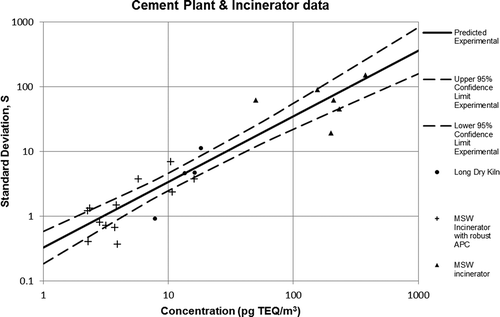
Figure 3. Relationship between standard deviation and concentration of cement plant and incinerator PCDD/PCDF data excluding possible outliers.

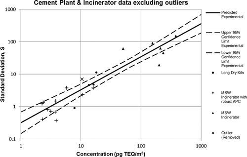
Figure 4. Relationship between standard deviation and concentration of cement plant and incinerator PCDD/PCDF data superimposed on the ReMAP relationship.

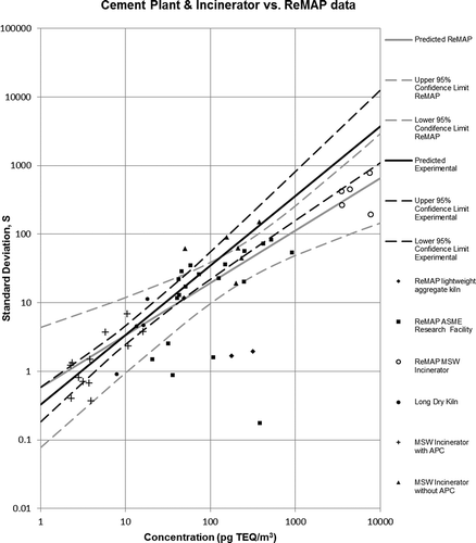
Figure 5. Relationship between standard deviation and concentration of cement plant and incinerator PCDD/PCDF data superimposed on the ReMAP relationship excluding possible outliers.

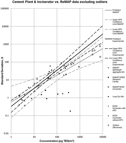
The plots show the means and confidence intervals of the relationships between standard deviations and concentrations for both simultaneous multiple and single train sampling data. The plots compare the results with and without possible outliers. Where the mean value fell outside of the confidence intervals created by the ReMAP data, it indicated that the standard deviation of the single train data was greater than that of the simultaneous multiple train data. This suggests that at a concentration greater than approximately 129 pg TEQ/m³, it would be beneficial to consider simultaneous multiple train sampling to confirm emissions values. When the possible outliers were excluded, the mean of the single train data moved outside the confidence limit at a lower concentration (111 pg TEQ/m³).

Discussion of Results

The results indicated that the variance was greater in the single train data than in simultaneous multiple train data for values above 129 pg TEQ/m³. At these values, there was benefit from the use of simultaneous multiple train sampling methods. This supports the hypothesis that the variability of data acquired from stack tests using a single train sampling method is greater than the variability of data acquired from simultaneous multiple train sampling. At concentrations below 129 pg TEQ/m³, there was no indication that there was a benefit from the use of simultaneous multiple train sampling. There were assumptions used in the analysis that may have contributed to the results, such as a slight difference between the single train and the simultaneous multiple train sampling and analysis procedures, oxygen correction was not conducted, and data from separate facilities were used.

The single train data were acquired from a long dry cement kiln and an MSW incinerator. Cement kilns operate at a high temperature and have long residence times. The high temperature and long residence time decrease the level of organic emissions, limiting the significance of the process variability on the PCDD/PCDF emissions. Twelve of the 18 MSW data points were acquired from the facility with a robust APC system installed. The robust APC system incorporated an SCR unit with both PAC and catalytic destruction. The APC system was added to the facility to greatly reduce organic emissions, which limited the significance of process variations affecting emissions. The consequence would be data that were affected by the variability of the sampling methods, with limited affect from the process variability of the facility. Six MSW data points were acquired before the robust APC system was installed. It appears that the data were affected by both process variability from the facility and variability from the sampling methods.

The simultaneous multiple trains used at the LWAK and MSW compliance-tested facility could not be inserted in the same openings in their respective stacks. The limitation was that the trains were inserted in ports 90° from one another. The probes would make each traverse separately, switching between traverses halfway through the sampling. The assumption used was that there would not be any process changes during the time it took to make the traverses. Although processes at industrial plants during stack sampling are held as constant as possible, there is a possibility that process changes could occur, increasing the variability in the results. As seen in Figure 4 and Figure 5, the APC system at the MSW incinerator that was used for single train data, high temperature, and residence time at the cement kiln may have decreased the variability. At low concentrations where the single train data were less affected by the process variability at the plant, the difference between the standard deviation of the single and simultaneous multiple train data was minimal. However, at higher concentrations where the organic emissions of the single train data were affected by both process and sampling variability, the standard deviation of the single train data becomes greater than that of the multiple train data, as can be seen in the range of concentrations from 100 to 300 pg TEQ/m³.

As can be observed from Figures 2 and 3, and Figures 4 and 5, the uncertainty of the standard deviation increased significantly at low concentrations. At low concentrations, the random error from the sampling method was significant, which in turn increased the variability. At concentrations below 129 pg TEQ/m³, the single train standard deviation was within the 95% confidence interval of the simultaneous multiple train data, and the simultaneous multiple train standard deviation was within the 95% confidence interval of the single train data. There was no benefit from the use of simultaneous multiple train sampling at concentrations below 129 pg TEQ/m³.

The ReMAP data were acquired and analyzed using EPA Method 23 (EPA, n.d.-b) and the cement plant and incinerator data using EC Method EPS 1/RM/2. The stack sampling procedure used for these methods was the same; however, the laboratory analysis procedure was slightly different. The laboratory procedure for the EC method requires that a sample be divided into four equal parts prior to being analyzed, one for PCDD/PCDF analysis, one for PCB/CB analysis, one for PAHs analysis, and one for archiving (Environment Canada, 1992). The EPA method gives the analyst the option to leave the sample whole, or to separate the sample into two parts, one to sample and one for archiving (EPA, n.d.-c). Variability from measurement error may have been introduced from separating the sample. Decreasing the sample size can increase error at low concentrations if the value was below the methods limit of quantification (Environment Canada, 1999) or approached the limit of detection (Rigo and Chandler, 1999). The differences in the procedure may have increased the variability in the EC EPS method when compared with the EPA method.

Figures 3 and 5 indicate data points that were either removed on the plot; this was due to the possibility that some data were outliers. To exclude possible outliers from the analysis, additional information from the source must be used to justify any conclusion that the data were not an accurate representation of the facilities emissions. This additional information was not available for this paper and the conclusions could not be drawn. Therefore, both analyses including and excluding the possible outliers were conducted to observe if any significant changes occurred in the results. If a data point was flagged as a possible outlier from the SPC outlier test, it was removed completely from the second plot. Dixon’s r test flags a value in a set of data (in this analysis a set of data consisted of three values). If one of these values in the set was flagged as an outlier, the standard deviation was calculated between the two other values. When the possible outliers were excluded, the relationship between the concentration and the standard deviation stays within the confidence limit of the ReMAP data to a lower concentration - 111 pg TEQ/m³. This result is not a practical concern because the limit for dioxins/furans emissions is generally below 100 pg TEQ/m³.

The oxygen data from sources in the ReMAP report were not available; therefore, the ReMAP data could not be oxygen corrected. Although there were oxygen data provided with the cement and incinerator data, it was not oxygen corrected to keep the procedure consistent between both the single and simultaneous multiple train data. Increased flow rate of air through a system dilutes the constituents of the flue gas. Oxygen correction prevents the possibility of the dilution effect by setting the oxygen levels of the data to an arbitrary amount. The variance of the ReMAP results could have been increased due to the inability to oxygen correct the data. The oxygen levels for the single train data did not vary significantly, and therefore would not have affected the results significantly.

Conclusion

The variance was greater in the single train data for values above 129 pg TEQ/m³. At these values, the benefit between the use of simultaneous multiple and single train sampling was increased precision. For values below 129 pg TEQ/m³, there was no indication that the variance was greater for the single train sampling method. For these values, it would not be beneficial to use simultaneous multiple train sampling methods because the precision does not improve from the use of single train sampling methods. The assumptions made and facilities that supplied the data may have contributed to the results, and it is not possible to conclude that differences between the simultaneous multiple and single train data were due to the different sampling methods.

Recommendations

Future comparisons between simultaneous multiple and single train sampling data are recommended. Samples should be acquired from a single facility. The laboratory methods between tests would be the same, and if the oxygen data are not obtained, the concentration should remain similar throughout the stack tests. This would reduce the sources of error and decrease the possibility that there are variables affecting a series of data that the other series of data are not affected by. Sampling times should be increased to the greatest time feasible, to decrease the chances that congeners are below the detection limit.

A comparison investigating the effect of different facility types and APC systems on the variability of single train and simultaneous multiple train PCDD/PCDF sampling is recommended. As explained in the discussion of the results, the significance of process variability on the emissions of dioxins/furans at certain facilities may be decreased due to the characteristics of the facility. It is possible that simultaneous multiple train sampling may be an effective method of increasing precision of dioxin/furan data at a specific type of facility, while being an ineffective method at others.

Funding

The authors wish to thank Carbon Management Canada, Queen’s University, and Lafarge Canada for supporting this work.

Additional information

Notes on contributors

Jamie Davis

Jamie Davis is a Master of Applied Science graduate student at Queen’s University, Kingston, Ontario.

Andrew Pollard

Andrew Pollard is a professor and the research chair in fluid dynamics and multi-scale phenomena at Queen’s University, Kingston, Ontario.

A. John Chandler

A. John Chandler, QEP, is president of A. J. Chandler & Associates Ltd., North York, Ontario.

References

- American Society of Mechanical Engineers Research Committee on Industrial and Municipal Waste. 1997. Retrofit of Waste-to-Energy Facilities Equipped with Electrostatic Precipitators. Research Report. New York: The American Society of Mechanical Engineers.
- Bryant, E.C. 1966. Statistical Analysis, 2nd ed. New York: McGraw-Hill.
- Burr, J.T. 2005. Elementary Statistical Quality Control, 2nd ed. New York: Marcel Dekker.
- Canadian Council of Ministers of the Environment. 2001. Canada-wide Standards for Dioxins and Furans. Winnipeg: CCME Council of Ministers.
- Chandra, M.J. 2001. Statistical Quality Control. Baco Raton, FL: CRC Press.
- Chang, M.B., K.H. Chi, S.H. Chang, and J.W. Yeh. 2007. Destruction of PCDD/Fs by SCR from flue gases of municipal waste incinerator and metal smelting plant. Chemosphere 66:1114–1122. doi:10.1016/j.chemosphere.2006.06.020
- Dixon, W.J., Jr., and F.J. Massey. 1969. Introduction to Statistical Analysis, 3rd ed. New York: McGraw-Hill.
- Environment Canada. 1992. Internal quality assurance requirements for the analysis of dioxins in environmental samples. http://www.ec.gc.ca/lcpe-cepa/default.asp?lang=En&n=5ED227EE-1 ( accessed March 12, 2014).
- Environment Canada. 1989. Reference Method for Source Testing: Measurement of Releases of Selected Semi-volatile Organic Compounds from Stationary Sources. http://www.ec.gc.ca/lcpe-cepa/default.asp?lang=En&n=942FC0FB-1(accessed March 12, 2014).
- Environment Canada. 1999. Level of Quantification Determination: PCDD/PCDF and Hexachlorobenzene. Canada: Analysis & Air Quality Division, Environmental Technology Centre.
- Fujii, T., T. Murakawa, N. Maeda, M. Kondo, K. Nagai, T. Hama, and K. Ota. 1994. Removal technology of PCDDs/PCDFs in FLUE GAS From MSW incinerators by fabric bag filter and SCR system. Chemosphere 29:2067–2070. doi:10.1016/0045-6535(94)90374-3
- Helsel, D.R.. n.d. KM Stats v1.5. http://www.practicalstats.com/nada/downloads_files/KMStats15.xls ( accessed March 3, 2014).
- Helsel, D.R. 2010. Summing nondetects: Incorporating low-level contaminants in risk assessment. Integr. Environ. Assess. Manage. 6:361–366. doi:10.1002/ieam.v6:3
- Karstensen, K.H. 2008. Formation, release and control of dioxins in cement kilns. Chemosphere 70:543–560. doi:10.1016/j.chemosphere.2007.06.081
- Lanier, W.S., and C.D. Hendrix. 2001. Reference Method Accuracy and Precision (ReMAP): Phase 1. Precision of Manual Stack Emissions Measurements. New York: American Society of Mechanical Engineers.
- Moffat, R.J. 1988. Describing the uncertainties in experimental results. Exp. Thermal Fluid Sci. 1:3–17. doi:10.1016/0894-1777(88)90043-X
- North Atlantic Treaty Organization Committee on the Challenges of Modern Society. 1988. Pilot Study on International Information Exchange on Dioxins and Related Compounds: Scientific Basis for the Development of the International Toxity Equivalency Factor (I-TEF) Method of Risk Assessment for Complex Mixtures of Dioxins and Related Compounds. http://nepis.epa.gov/Exe/ZyNET.exe/900F0800.TXT?ZyActionD=ZyDocument&Client=EPA&Index=1986+Thru+1990&Docs=&Query=&Time=&EndTime=&SearchMethod=1&TocRestrict=n&Toc=&TocEntry=&QField=&QFieldYear=&QFieldMonth=&QFieldDay=&IntQFieldOp=0&ExtQFieldOp=0&XmlQuery=&File=D%3A%5Czyfiles%5CIndex%20Data%5C86thru90%5CTxt%5C00000016%5C900F0800.txt&User=ANONYMOUS&Password=anonymous&SortMethod=h%7C-&MaximumDocuments=1&FuzzyDegree=0&ImageQuality=r75g8/r75g8/x150y150g16/i425&Display=p%7Cf&DefSeekPage=&SearchBack=ZyActionL&Back=ZyActionS&BackDesc=Results%20page&MaximumPages=1&ZyEntry=1&SeekPage=x&ZyPURL
- Ontario Ministry of the Environment. 2004. Guideline A-8: Guildine for the Implementation of Canada-wide Standard for Emissions of Mercury and of Dioxins and Furans. http://www.ene.gov.on.ca/stdprodconsume/groups/lr/@ene/@resources/documents/resource/std01_079113.pdf ( accessed February 22, 2014).
- Ontario Ministry of the Environment. 2009. Ontario Source Testing Code. http://www.ene.gov.on.ca/stdprodconsume/groups/lr/@ene/@resources/documents/resource/stdprod_080763.pdf ( accessed March 12, 2014).
- Rigo, G., and J. Chandler. 1999. Quantification limits for Reference Methods 23, 26, and 29. J. Air Waste Manage. Assoc. 49:399–410. doi:10.1080/10473289.1999.10463819
- U.S. Environmental Protection Agency. n.d.-a. Clean Air Act National Stack Testing Guidance. http://www.epa.gov/compliance/resources/policies/monitoring/caa/stacktesting.pdf ( accessed March 12, 2014).
- U.S. Environmental Protection Agency. n.d.-b. Method 23—Determination of Polychlorinated Dibenzo-p-dioxins and Polychlorinated Dibenzofurans from Municipal Waste Combustors. http://www.epa.gov/ttnemc01/promgate/m-23.pdf ( accessed March 12, 2012).
- U.S. Environmental Protection Agency. n.d.-c. National Functional Guidelines for Chlorinated Dioxin/Furan Data Review. A report prepared by the U.S. Environmental Protection Agency as part of the National Contract Laboratory Program. http://www.epa.gov/superfund/programs/clp/guidance.htm ( accessed March 3, 2014).