A two-step approach for relating tapered element oscillating microbalance and dichotomous air sampler PM_2.5 measurements

Abstract

A method for transforming continuous monitoring (CM) fine particulate matter (aerodynamic diameter <2.5 μm; PM_2.5) data (i.e., by tapered element oscillating microbalance [TEOM]) obtained from the Canadian National Air Pollution Surveillance (NAPS) program to meet the data quality objective (DQO) of R² > 0.8 against the co-located federal reference method (i.e., dichotomous air sampler) is described. By using a two-step linear regression to account for the effect of the ambient temperature, 16 out of the 23 examined sites met the common model adequacy threshold of R² > 0.8. After the transformation, 20 out of the 23 examined sites met the DQO of R² > 0.7, as recommended by the U.S. Environmental Protection Agency (EPA). A combined two-step statistical approach was also examined and revealed similar results. The methods described herein show that the CM data can be successfully transformed to meet DQOs for representative sites across Canada using year-round (both summer and winter) data.

Implications:

This study provides a transformation approach to correct ambient TEOM data against the federal reference method without dividing the ambient data according to warm and cold seasons. This transformation approach will significantly improve the correlation coefficient between TEOM and dichotomous air sampler data. It is possible that TEOM data at many Canadian locations can be transformed to meet the EPA data quality objective, thus making this transformation approach useful for comparisons of ambient PM data across jurisdictions.

Introduction

The tapered element oscillating microbalance (TEOM) provides hourly ambient particulate matter data (Patashnick and Rupprecht, 1991) and is widely used across Canada as the result of the establishment of the Canada-wide Standards (CWS) for Particulate Matter (PM) and Ozone. The CWS for PM and Ozone agreement was signed in June 2000 and committed the provincial and territorial governments, except Quebec, to achieve the PM_2.5 (aerodynamic diameter <2.5 μm) and ozone standards of 30 μg/m³ over 24 hr and 65 ppb over a daily 8-hr maximum, respectively, by 2010 (Canada-wide Standards Development Committee for Particulate Matter [PM] and Ozone, 1999). To achieve this reporting protocol, jurisdictions are required to report the annual 98^th percentile PM_2.5 daily levels averaged over 3 yr.

In the United States, the U.S. Environmental Protection Agency (EPA) allows the use of non–federal reference method instruments, such as the TEOM, for reporting the air quality index (AQI) as long as a linear relationship between the two methods is established by linear regression with a statistically significant correlation coefficient (Eberly et al., 2002). In this type of regression (single variable), the coefficient of determination (R²) is measured as the square of the correlation coefficient (R) between the continuous PM monitor and the federal reference method and forms the foundation for developing the data quality objective (DQO) for the continuous PM monitor. The EPA has deemed an acceptable R² value to equal 0.70 (correlation [R] of 0.84) (Eberly et al., 2002). However, a common model adequacy threshold has been recommended to be R² > 0.80 (Eberly et al., 2002).

Previous studies have compared TEOM results with the manual, 24-hr, filter-based reference methods that use gravimetric analysis, such as the dichotomous (dichot) samplers (Chung et al., 2001; Schwab et al., 2006; Meyer et al., 2000; Vega et al., 2003). The results showed discrepancies between the measurements obtained by the TEOM and dichot samplers, especially during the winter months (Allen et al., 1997; Ayers et al., 1999). Since the dichot operates at ambient temperatures, warmer summer months compare better with the TEOM (operating at 30 or 40 °C) than during the winter months (Hauck et al., 2004). These discrepancies have been attributed to artefacts related to semivolatile materials (SVMs), such as the loss of semivolatile organic compounds (SVOCs), particle-bound water, and ammonium nitrate (Eatough et al., 2003; Tanner and Parkhurst, 2000; Rees et al., 2004).

Several studies have examined the use of a correction model to adjust the TEOM measurements to meet the DQO set out by regulatory agencies (Rizzo et al., 2003; Kashuba and Scheff, 2008). This is of particular interest for jurisdictions in a northern climate, since colder winter months bring the highest discrepancies between the TEOM and dichot. Other studies have examined the correlation between the TEOM and other federal equivalent method (FEM) instruments, such as the SHARP 5030, in order to determine the differences and similarities between the two systems (Sofowote et al., 2014). In the Sofowote et al. study, the transformed TEOM data were then compared with the federal reference method and showed improvement during the fall and winter months.

In Canada, a report prepared by George Allen (Allen Report) was published for the National Air Pollution Surveillance (NAPS) program run by Environment Canada in 2010 evaluating transformation methods to adjust historical TEOM data in the NAPS network to meet a R² > 0.80 DQO (Allen, 2010). Data were obtained from 23 sites across Canada with at least 100 days of collocated NAPS Canadian federal reference method (FRM) and TEOM data. The data were then split into warmer (>10 °C) and colder (<10 °C) seasons and assessed separately. The results confirmed the increased discrepancies due to the cold weather; thus, separating data sets into warmer and colder seasons improved the correlation coefficient. However, the studies showed no meaningful correlation between TEOM PM loss with ambient temperature, nor was any additional improvement seen with the use of more complex temperature-based approaches (Allen, 2010). The Allen Report also tested the use of three regional pooled regressions to generate regional transformation factors. The resulting correlations were reasonable for Quebec-Ontario (R² = 0.84) and British Columbia (R² = 0.82), but only marginally useful for The Prairies (R² = 0.68).

In this study, a two-step transformation approach is used to improve the correlation (R²) between TEOM and FRM (dichotomous) measurements without subdividing the data set into “warmer” and “colder” seasons. First, the temperature influence was determined and the TEOM data were transformed to remove the temperature effects. Then, the transformed TEOM data were correlated with FRM measurements to generate the second transformation factor for each individual site. The results show that by using this two-step approach, it is possible to transform the TEOM measurements with improved R² such that the data meet the DQOs. The advantage for developing transformation methodology for PM_2.5 data is to provide a way to compare data from various continuous and filter-based air monitors, particularly when analyzing PM_2.5 data across different jurisdictions and seasons.

Methodology

Data

Daily FRM and TEOM PM_2.5 data sets used by the Allen Report were obtained from the NAPS Web site. The data sets also have the associated daily maximum and minimum temperatures. Table 1 shows the locations and the number of records available for this study as well as the summary statistics of the data. Data from selected locations had minor revisions after the Allen Report was published. The impact of those minor revisions will be discussed in Results and Discussions. The data were first screened for outliers using the following steps:

Table 1. List of the NAPS collocated sites, number of measurement records, and measurement intervals

	No. of	Interval		TEOM (μg/m^3)		FRM (μg/m^3)		Temperature (°C)
Site	Records	From	To	Mean	SD	Mean	SD	Mean	SD
Fredricton NB	146	2005	2009	4.83	2.83	6.71	3.49	10.83	12.34
St Anicet QC	207	2005	2007	7.45	5.43	8.80	5.86	14.42	12.64
St Jean QC	194	2005	2007	7.04	5.16	9.49	6.65	14.95	11.75
Ottawa ON	508	2005	2009	6.50	4.56	8.23	5.29	11.89	12.44
Winsor ON	238	2005	2008	10.04	6.60	11.84	6.38	16.17	11.67
Toronto Elmcrest ON	344	2005	2008	8.43	6.27	10.77	6.89	12.46	11.59
Toronto Etona ON	153	2005	2008	8.71	5.17	10.26	5.62	14.26	11.36
Toronto Resource ON	526	2005	2008	8.18	5.88	10.54	6.72	14.10	11.05
Hamilton ON	202	2005	2009	8.61	5.46	11.35	6.36	12.08	11.77
Simcoe ON	304	2005	2008	8.69	6.68	10.69	6.88	14.01	11.31
Essex ON	256	2005	2008	7.39	5.50	11.25	7.03	9.25	11.25
Winnipeg MB	188	2005	2009	4.40	2.32	6.49	2.90	10.00	14.77
Saskatoon SK	132	2005	2009	4.00	1.86	6.64	2.85	11.39	13.23
Edmonton AB	108	2008	2008	5.36	3.17	8.43	5.36	9.30	13.54
Calgary AB	101	2006	2008	6.13	2.65	6.71	3.29	9.55	11.99
Van-Port Moody BC	181	2005	2009	5.90	3.05	6.94	3.10	14.21	6.55
Van-Burnaby BC	411	2005	2009	5.01	3.16	6.40	3.35	16.20	7.24
Prince George BC	147	2008	2009	7.57	6.50	9.82	7.42	10.70	11.42
Victoria BC	115	2005	2009	5.37	2.72	7.41	3.93	14.63	7.03
Van-Abbotsford	326	2005	2008	5.02	2.82	7.13	3.34	16.00	7.35
Quesnel BC	172	2007	2009	6.54	3.91	8.91	5.20	9.73	12.35
Williams Lake BC	85	2005	2006	7.32	4.44	9.60	5.37	8.84	10.64
Golden BC	136	2005	2007	6.91	3.89	10.50	7.19	19.10	7.11

1. Data points with missing values for either TEOM or FRM measurements were removed from the data set.

2. All data points with TEOM measurements more than 2 times greater than the FRM measurements were deleted from the data set.

3. A simple linear regression line was fitted to the FRM measurements as functions of the TEOM measurements, and all data points with regression errors greater than 3 times the standard error of the simple linear regression line were deleted.

Further information on the TEOM operating temperature by site is available in Supplementary Material, Table S1.

Data analysis

Two-step linear regression

The two-step derivation process assumes that the discrepancies between TEOM and FRM measurements are due to (1) random instrument- and/or measurement error–induced discrepancy, and (2) temperature-induced discrepancy. The random instrument discrepancy is caused by factors such as system setup, sampling procedures, equipment malfunctions, and operational error. The differences between the TEOM and FRM measurements, both taken at the operational temperature of the TEOM, are examples of system discrepancy, since the temperature-induced discrepancies are not expected in such circumstances. The concept of temperature-induced discrepancy, especially in the winter months, is based on the following assumptions:

1. The discrepancy is due to the evaporation of semi volatiles (“evaporable” mass) at the TEOM operating temperature (30 or 40 °C).

2. The “evaporable” semivolatiles are condensed onto the particulate matter at low ambient temperatures (e.g., cold season).

3. The amount of “evaporable” mass is proportional to the PM mass as measured by the TEOM.

4. The portion of “evaporable” mass is unique for each individual site, and to a lesser degree, warm and cold seasons.

Based on the temperature-induced discrepancy assumptions, the relationship between TEOM and FRM measurements can be expressed as the following:

1

where FRM is the measurement collected by the federal reference method (dichot), CM is the measurement obtained by the continuous method (TEOM), β×CM×T is the contributing factor of “evaporable” mass, T is the ambient temperature expressed either as the daily maximum temperature or daily minimum temperature, and α and β are regression parameters that are unique to each site. In eq 1, the CM term refers to the measured contribution from the TEOM only, whereas the β×CM×T takes into consideration the evaporable/condensable material formed on the surface of the PM at the ambient temperature.

Equation 1 can be rewritten as

2

where ϵ is the residual error due to the system discrepancies, Ra is the ratio FRM/CM, and α and β are regression parameters, representing the intercept and slope, respectively, of the linear regression of Ra on T. Equation 2 was fitted to the data for each site to obtain the estimates ( and ) of the slope and intercept (β and α), respectively (see Figures 1 to 5) using the regression procedure in SAS version 9.3 (SAS Institute Inc., 2011).

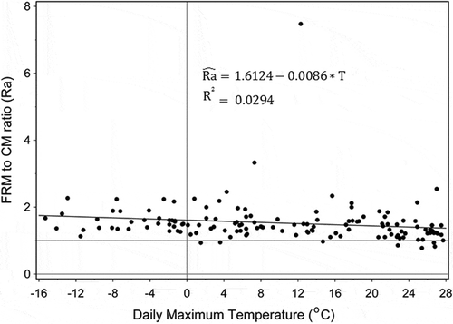
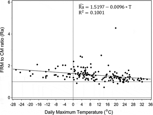
Figure 1. Correlation between FRM/CM ratio and daily maximum temperature for Fredericton NB (site no. S40103).

The goal of this process is to find a way to transform the CM into a new value (CM’) that meets the DQO objective by removing the temperature effect. Thus, the CM’ is obtained via eq 2ʹ by multiplying each CM value by the term () obtained from the above.

2’

A linear regression equation of the resulting CM’ on the original FRM results ( eq 2) is then fitted to evaluate the new R² against the DQO.

3

From eq 3, m is the slope of the new regression equation, which is expected to be much closer to 1, and b is the intercept, which is expected to approach 0 (see Figures 6 to 10).

The two-step approach is expected to improve the correlation between FRM and transformed CM by taking into consideration the temperature influence and the local “evaporable” mass contributing factor.

Combined two-step linear statistical approach

The second approach involves fitting a linear regression of FRM on the CM, daily maximum temperature (T), and the interaction of daily maximum temperature and CM:

4

where β₀ is the intercept, β₁ is the slope with respect to CM, β₂ is the slope with respect to T, CM×T is the interaction term for the CM and the daily maximum temperature (T), and β₃ is the slope with respect to the interaction term (CM×T). This approach will be referred to as the “combined two-step statistical approach.” Compared with the separate two-step linear regression described above (see eq 1), β₀ and β₂T are added terms. The β₂T term was added to test the impact of temperature alone on the discrepancy between FRM and CM. β₀ is an additional parameter that gives eq 4 more flexibility than eq 1. The analysis shows that whereas β₀ was statistically significant in most cases when tested at the 5% probability level, β₂ was not significant in most cases (see Table 5).

Results and Discussion

Comparison with the results of the Allen Report

A simple linear regression analysis was performed for all the sites using the whole NAPS data set, with outliers removed as described previously, to verify the results of the Allen Report and to show that any gain in correlation resulting from this study are not data driven. Table 2 summarizes the results of the regression of FRM on CM. The intercept, slope, and R² values are shown, along with the R² values previously reported by the Allen Report. In general, the correlations (R²) are similar; however, there are some minor discrepancies for St Jean QC, Winnipeg MB, Edmonton AB, Calgary AB, and Victoria BC. According to NAPS data managers, data sets from those locations had minor revisions after the Allen Report was published (personal communication) due to further data quality assurance/quality control (QA/QC) corrections. Also, the outliers that were removed in this study during data evaluation may also have contributed to the slight differences observed.

Table 2. Comparison of the regression coefficients and coefficients of determination for the NAPS sites

		Coefficients
Site	Site ID	Intercept (b)	Slope (m)	Coefficient of Determination (R^2)	Coefficient of Determination (R^2) from Allen et al. (2010)
Fredericton NB	S40103	0.0651	0.7053	0.790	0.789
St Anicet QC	S54401	−0.4227	0.8910	0.883	0.883
St Jean QC	S55301	2.4648	0.4666	0.411	0.622
Ottawa ON	S60104	−0.2029	0.8094	0.852	0.842
Winsor ON	S60211	−0.4312	0.8586	0.779	0.779
Toronto Elmcrest ON	S60413	−0.5908	0.8312	0.859	0.845
Toronto Etona ON	S60429	−0.1823	0.8502	0.842	0.839
Toronto Resource ON	S60430	−0.1799	0.7911	0.783	0.755
Hamilton ON	S60512	−0.2120	0.7832	0.807	0.807
Simcoe ON	S62601	−1.0242	0.8901	0.883	0.883
Essex ON	S65601	−0.5851	0.7409	0.759	0.735
Winnipeg MB	S70119	0.9687	0.5395	0.532	0.499
Saskatoon SK	S80211	1.1442	0.4383	0.365	0.365
Edmonton AB	S90132	1.0511	0.5106	0.745	0.466
Calgary AB	S90227	1.8617	0.6675	0.559	0.225
Van-Port Moody BC	S100111	−0.4115	0.8978	0.837	0.837
Van-Burnaby BC	S100119	−0.7264	0.8974	0.868	0.846
Prince George BC	S100202	−0.1059	0.7754	0.818	0.818
Victoria BC	S100304	1.4213	0.5225	0.628	0.445
Van-Abbotsford	S101004	−0.2465	0.7365	0.664	0.645
Quesnel BC	S101701	0.0607	0.7390	0.895	0.895
Williams Lake BC	S102701	0.1630	0.7306	0.667	0.642
Golden BC	S103202	1.6186	0.5145	0.790	0.789

Note: The coefficients of determination (R²) for the same regression model presented in Allen (2010) are included.

A close examination of Table 2 shows that the correlation factor varies greatly from R² = 0.4113 to R² = 0.8950 for St Jean QC and Quesnel BC, respectively. A similar wide range of values is also observed for the slope and intercept. If there was perfect correlation between the FRM and CM readings, the correlation and slope would be close to 1 and the intercept would be close to 0. These results clearly show that although in some cities there are good correlations, in other cities the CM readings are poorly correlated to the FRM readings. These discrepancies and poor correlations between CM and FRM readings occur across the country and may be due to variety of reasons such as seasonal variations and the presence of semivolatiles.

Correlation between the FRM/CM ratio and ambient temperature (step 1)

For the first step in the transformation, the Ra (or FRM/CM ratio) is plotted against the maximum daily temperature. Figure 1 illustrates this type of plot for the maximum daily temperature obtained for Fredericton NB (site S40103). As the daily maximum temperature increases along the x-axis, the Ra ratio decreases and appears to approach the value of 1 at the daily maximum temperature of around 30 °C. This pictorial representation shows that there is better agreement between FRM and CM during warmer temperatures.

Similar plots are shown in Figures 2–5 for Toronto Etona ON, Saskatoon SK, Edmonton AB, and Quesnel BC, respectively, representing unique regions across Canada. Other locations across Canada also reveal similar plots, with the Ra ratio approaching 1 at warmer temperatures. Qualitatively, in cities such as Saskatoon SK and Edmonton AB, the Ra ratio shows stronger discrepancies, with the ratio approaching 3 during the coldest temperatures, possibly due to the combination of cold winter and the presence of semivolatiles. For cities with a warmer winter, the Ra ratio is closer to 2.

Figure 2. Correlation between FRM/CM ratio and daily maximum temperature for Toronto Etona ON (site no. S60429).

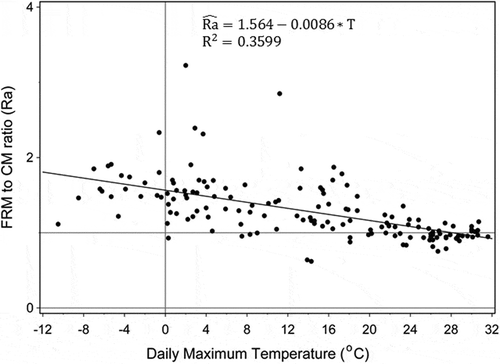
Figure 3. Correlation between FRM/CM ratio and daily maximum temperature for Saskatoon SK (site no. S80211).

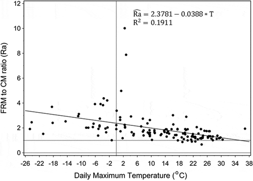
Figure 4. Correlation between FRM/CM ratio and daily maximum temperature for Edmonton AB (site no. S90132).

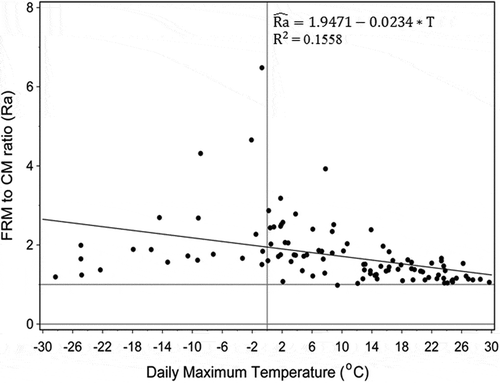
Figure 5. Correlation between FRM/CM ratio and daily maximum temperature for Quesnel BC (site no. S101701).

The slope and intercept were obtained for the complete data set, including summer and winter months, where the Ra ratio was plotted against the daily maximum temperature. Table 3 summarizes the data. The slopes have a negative value for all sites except Williams Lake BC, showing that there is more agreement in the Ra ratio during warmer weather. There is also a wide range of y-intercepts, ranging from 1.2 to 2.4. The R² values are consistently higher when daily maximum temperatures are used as opposed to using daily minimum temperatures, except for Edmonton AB and Williams Lake BC.

Table 3. Regression coefficients and coefficients of determination (R²) for the FRM/CM ratio calculated using the daily minimum and daily maximum temperatures

			Maximum Daily Temperature			Minimum Daily Temperature
Site	Site ID	Intercept	Slope	R^2	Intercept	Slope	R^2
Fredericton NB	S40103	1.6124	−0.0086	0.0294	1.5179	−0.0032	0.0035
St Anicet QC	S54401	1.4263	−0.0102	0.1262	1.3397	−0.0099	0.0998
St Jean QC	S55301	2.2792	−0.0425	0.1053	1.8855	−0.0396	0.0755
Ottawa ON	S60104	1.6744	−0.0162	0.0212	1.5144	−0.0131	0.0119
Winsor ON	S60211	1.7775	−0.0264	0.3740	1.5880	−0.0293	0.3615
Toronto Elmcrest ON	S60413	1.6918	−0.0221	0.2266	1.5163	−0.0228	0.1783
Toronto Etona ON	S60429	1.5654	−0.0086	0.3599	1.4131	−0.0213	0.3080
Toronto Resource ON	S60430	1.7273	−0.0194	0.0925	1.5659	−0.0194	0.0718
Hamilton ON	S60512	1.7962	−0.0266	0.2660	1.5638	−0.0267	0.2067
Simcoe ON	S62601	1.6600	−0.0191	0.1808	1.4900	−0.0193	0.1357
Essex ON	S65601	2.0450	−0.0337	0.2883	1.7616	−0.0369	0.2715
Winnipeg MB	S70119	1.9719	−0.0239	0.1415	1.7101	−0.0216	0.0989
Saskatoon SK	S80211	2.3781	−0.0388	0.1911	1.9025	−0.0432	0.1723
Edmonton AB	S90132	1.9471	−0.0234	0.1558	1.7191	−0.0277	0.1651
Calgary AB	S90227	1.2387	−0.0117	0.1897	1.0988	−0.0115	0.1359
Van-Port Moody BC	S100111	1.4218	−0.0100	0.0321	1.3313	−0.0066	0.0101
Van-Burnaby BC	S100119	1.6736	−0.0166	0.0624	1.4792	−0.0109	0.0130
Prince George BC	S100202	1.5450	−0.0089	0.0506	1.4460	−0.0060	0.0176
Victoria BC	S100304	1.7475	−0.0179	0.0658	1.6056	−0.0192	0.0440
Van-Abbotsford	S101004	2.4554	−0.0433	0.0643	1.9501	−0.0271	0.0131
Quesnel BC	S101701	1.5197	−0.0096	0.1001	1.4053	−0.0089	0.0582
Williams Lake BC	S102701	1.3508	0.0099	0.0246	1.4563	0.0154	0.0448
Golden BC	S103202	1.7782	−0.0216	0.1310	1.4472	−0.0137	0.0238

Note: This is the step 1 of the two-step approach.

Correlation between FRM and CM’

As described in eq 2’, the slope and intercept from Table 3 were used to develop a new transformed continuous monitoring value (CM’), which essentially transforms the CM into a new term with the temperature dependence accounted for. When the transformed CM’ is plotted against the FRM values, the resulting slope (m) and y-intercept (b) should approach 1 and 0, respectively.

Figure 6. Correlation between FRM and CM’ for Fredericton NB (site no. S40103).

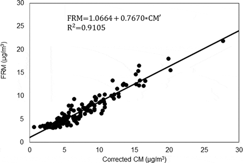
Figures 6–10 compare the new transformed CM’ values with the observed FRM data for the cities of Fredericton NB, Toronto Etona ON, Saskatoon SK, Edmonton AB, and Quesnel BC, respectively. The results show improved agreement using the corrected CM’ data compared with the uncorrected data. The five graphs demonstrate the slope of the graphs now approach closer to 1.

Figure 7. Correlation between FRM and CM’ for Toronto Etona ON (site no. S60429).

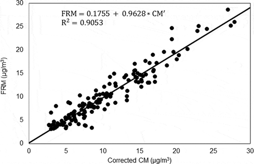
Figure 8. Correlation between FRM and CM’ for Saskatoon SK (site no. S80211).

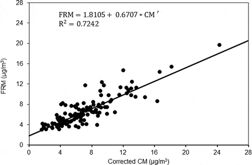
Figure 9. Correlation between FRM and CM’ for Edmonton AB (site no. S90132).

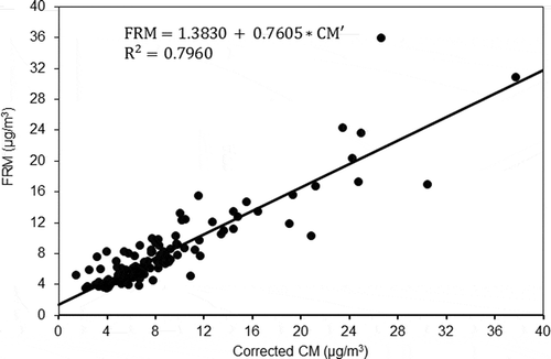
Figure 10. Correlation between FRM and CM’ for Quesnel QC (site no. S101701).

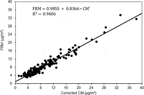
Table 4 summarizes the data comparing the newly transformed CM’ plotted against the FRM, and the resulting slope and y-intercept. Comparison of the newly transformed R² values against the R² values obtained from the conventional linear regression show at least some improvement for almost all the sites except for Williams Lake BC. This exception is likely due to the Ra versus temperature graph having a positive slope for Williams Lake BC, which is not consistent with the four assumptions given in Data Analysis. After the transform, six more sites, including Fredericton NB, Windsor ON, and Golden BC, now meet the DQO objective of R² >0.8. However, there are still some notable sites that do not meet the DQO criteria, namely, the prairie cities such as Winnipeg MB, Saskatoon SK, and Calgary AB where the winters are colder, and some BC cities. However, most cities showed significant improvements in R², with almost all cities meeting the R² DQO of >0.7, as recommended by the EPA. The exceptions are St Jean QC, Winnipeg MB, and Williams Lake BC (R² below 0.7). After the first transformation correcting for ambient temperature, the values of the slope for all sites have improved significantly with the slope approaching one (see Table 4).

Table 4. Regression coefficients and coefficients of determination (R²) for the corrected CM using the daily maximum temperature

		Coefficients		R^2
Site	Site ID	Intercept (b)	Slope (m)	Before Transformation	After Transformation
Fredericton NB	S40103	1.066	0.767	0.789	0.910
St Anicet QC	S54401	0.567	0.890	0.882	0.938
St Jean QC	S55301	1.557	0.731	0.411	0.615
Ottawa ON	S60104	0.681	0.811	0.852	0.920
Winsor ON	S60211	0.515	0.929	0.779	0.899
Toronto Elmcrest ON	S60413	0.043	0.971	0.858	0.940
Toronto Etona ON	S60429	0.176	0.963	0.842	0.905
Toronto Resource ON	S60430	0.541	0.914	0.783	0.879
Hamilton ON	S60512	1.062	0.865	0.806	0.843
Simcoe ON	S62601	0.558	0.903	0.882	0.947
Essex ON	S65601	1.207	0.835	0.759	0.849
Winnipeg MB	S70119	1.719	0.655	0.531	0.624
Saskatoon SK	S80211	1.811	0.671	0.365	0.724
Edmonton AB	S90132	1.383	0.761	0.744	0.796
Calgary AB	S90227	0.149	0.962	0.559	0.754
Van-Port Moody BC	S100111	1.092	0.798	0.836	0.906
Van-Burnaby BC	S100119	1.115	0.757	0.868	0.912
Prince George BC	S100202	1.823	0.720	0.817	0.943
Victoria BC	S100304	0.701	0.867	0.627	0.757
Van-Abbotsford	S101004	1.755	0.661	0.663	0.760
Quesnel BC	S101701	0.986	0.837	0.895	0.940
Williams Lake BC	S102701	2.503	0.637	0.667	0.584
Golden BC	S103202	0.745	0.849	0.789	0.856

Note: This is the step 2 of the two-step approach.

Correlation between FRM and CM using the combined two-step regression

Table 5 shows the results between FRM and CM using the combined two-step regression. Compared with the two-step linear regression approach (Table 4), the R² values are similar. The β₃ values are consistently negative, showing there is a negative correlation between FRM and the CM×T interaction, which is consistent with the negative slope values observed in Table 3. β₂ have mixed values, showing both positive and negative correlations between FRM and the ambient temperature. Further statistical analyses as shown in Table 5 reveal β₂ to be statistically insignificant (at 5% probability) for most cases. Similar observations were found in Rizzo et al. (2003). This supports the assumption of this study that proposes that temperature alone does not fully explain the discrepancies between the FRM and CM measurements, although the temperature effect plays a major role. The amount of volatiles condensed onto the PM can also affect the discrepancies between FRM and CM. The ambient temperature impact on FRM/CM discrepancies should be considered in conjunction with the ambient PM levels (e.g., CM readings).

Table 5. Regression coefficient and probability of significance (PS) for the combined two-step statistical approach

Site		Intercept		Slope for CM		Slope for T		Slope for CM×T
Number	Site	β0	PS	β1	PS	β2	PS	β3	PS	R^2
S40103	Fredricton NB	1.2578	0.0001	1.1819	0.0000	−0.0092	0.6099	−0.0033	0.2574	0.8710
S54401	St Anicet QC	0.6170	0.0480	1.2560	0.0000	0.0104	0.5148	−0.0099	0.0000	0.9273
S55301	St Jean QC	1.5823	0.1012	1.7480	0.0000	−0.0879	0.0723	−0.0244	0.0000	0.7077
S60104	Ottawa ON	0.4416	0.0113	1.3704	0.0000	0.0225	0.0205	−0.0143	0.0000	0.9331
S60211	Winsor ON	1.3195	0.0152	1.4956	0.0000	−0.0485	0.0705	−0.0164	0.0000	0.8726
S60413	Toronto Elmcrest ON	0.2129	0.4042	1.6101	0.0000	−0.0045	0.7601	−0.0202	0.0000	0.9467
S60429	Toronto Etona ON	−0.1401	0.7719	1.5685	0.0000	0.0039	0.8734	−0.0208	0.0000	0.9347
S60430	Toronto Resource ON	1.0126	0.0081	1.4625	0.0000	0.0083	0.6815	−0.0168	0.0000	0.8470
S60512	Hamilton ON	1.3824	0.0035	1.4446	0.0000	−0.0495	0.0604	−0.0136	0.0000	0.8946
S62601	Simcoe ON	1.2899	0.0000	1.3624	0.0000	−0.0355	0.0284	−0.0112	0.0000	0.9394
S65601	Essex ON	1.6271	0.0001	1.6259	0.0000	−0.0585	0.0274	−0.0205	0.0000	0.8701
S70119	Winnipeg MB	0.9854	0.0329	1.5089	0.0000	0.0232	0.3597	−0.0213	0.0000	0.6269
S80211	Saskatoon SK	2.8498	0.0000	1.2820	0.0000	−0.0180	0.5744	−0.0203	0.0030	0.5979
S90132	Edmonton AB	1.3548	0.0093	1.4819	0.0000	−0.0627	0.0967	−0.0056	0.2767	0.8094
S90227	Calgary AB	−0.3838	0.5544	1.2868	0.0000	0.0812	0.0493	−0.0232	0.0000	0.7175
S100111	Van-Port Moody BC	0.9371	0.0466	1.1051	0.0000	0.0313	0.3038	−0.0096	0.0136	0.8470
S100119	Van-Burnaby BC	1.1421	0.0000	1.1937	0.0000	0.0010	0.9444	−0.0087	0.0000	0.9098
S100202	Prince George BC	2.0689	0.0000	1.0973	0.0000	−0.0102	0.6490	−0.0068	0.0003	0.9418
S100304	Victoria BC	0.4445	0.6413	1.6221	0.0000	0.0260	0.6763	−0.0234	0.0109	0.7256
S101004	Van-Abbotsford	3.2347	0.0000	0.9561	0.0000	−0.0501	0.0679	−0.0004	0.9082	0.6751
S101701	Quesnel BC	1.3080	0.0000	1.2537	0.0000	−0.0219	0.1915	−0.0073	0.0000	0.9374
S102701	Williams Lake BC	2.0519	0.0205	0.9980	0.0000	0.0200	0.7725	−0.0019	0.7633	0.7427
S103202	Golden BC	0.2252	0.8242	1.6238	0.0000	0.0477	0.3620	−0.0279	0.0000	0.8439

Conclusion

The two methods described in this paper are successful in removing the temperature dependence from the CM data set obtained from the NAPS program. The results showed that by using this process, the CM data set could be transformed such that the correlation coefficient (R²) improves. Of the 23 sites analyzed, an improvement in the R² value was seen for all sites except for one (Williams Lake BC). In the original one-step transformation (Allen et al., 2010), 10 out of the 23 sites met the DQO of R² > 0.8. After the two-step transformation outlined in this paper, 16 out of the 23 sites met the DQO of R² > 0.8, and 20 sites met the EPA-recommended DQO of R² > 0.7. Using the combined two-step regression, similar results are obtained. Based on R² values, the two-step regression performs slightly better than the combined two-step regression.

The analyses discussed in this paper reveal that the differences between the FRM and CM show correlation with the ambient temperature. By accounting for the effect of the ambient temperature, the data can be transformed to meet the EPA-recommended DQO of R² > 0.7 for all evaluated sites, except three (St Jean QC, Winnipeg MB, and Williams Lake BC).

Abbreviations

New BrunswickNB

QuebecQC

OntarioON

ManitobaMB

SaskatchewanSK

AlbertaAB

British ColumbiaBC

Supplemental Material

Supplemental data for this article can be accessed at http://dx.doi.org/10.1080/10962247.2014.934484.

Acknowledgment

The authors would like to thank the Environment Canada National Air Pollution Surveillance Network for providing the data used in this paper, and Yang Chen and Tengzhou Lun for assistance with data analysis and validation. The authors are grateful for the useful comments from the three reviewers and constructive suggestions from Dr. Allan Legge and Dr. Rongcai Yang.

Additional information

Notes on contributors

Long Fu

Long Fu is a science manager with the Alberta Environmental Monitoring, Evaluation and Reporting Agency, Edmonton, Alberta, Canada.

Thompson Nunifu

Thompson Nunifu is an environmental statistician and Bonnie Leung is an analytical chemist with Alberta Environment and Sustainable Resource Development, Edmonton, Alberta, Canada.

Bonnie Leung

Thompson Nunifu is an environmental statistician and Bonnie Leung is an analytical chemist with Alberta Environment and Sustainable Resource Development, Edmonton, Alberta, Canada.

References

- Allen, G. 2010. Evaluation of Transformation Methods for Adjusting Historical TEOM Data in the NAPS Network. Prepared for the Analysis and Air Quality Section, Environment Canada, Ottawa, Ontario, Canada.
- Allen, G., C. Sioutas, P. Koutrakis, R. Reiss, F.W. Luhrmann, and P.T. Roberts. 1997. Evaluation of the TEOM® method for measurement of ambient particulate mass in urban areas. J. Air Waste Manage. Assoc. 47:682–689. doi:10.1080/10473289.1997.10463923
- Ayers, G.P., M.D. Keywood, and J.L. Gras. 1999. TEOM vs. manual gravimetric methods for determination of PM2.5 aerosol mass concentrations. Atmos. Environ. 33:3717–3721. doi:10.1016/S1352-2310(99)00125-9
- Canada-wide Standards Development Committee for Particulate Matter (PM) and Ozone. 1999. Discussion paper on PM and ozone. Canada-wide Standards Scenarios for Consultation. http://www.ccme.ca/assets/pdf/pmozone_standard_e.pdf (accessed July 24, 2013).
- Chung, A., D.P.Y. Chang, M.J. Kleeman, K.D. Perry, T.A. Cahill, D. Dutcher, E.M. McDougall, and K. Stroud. 2001. Comparison of real-time instruments used to monitor airborne particulate matter. J. Air Waste Manage. Assoc. 51:109–120. doi:10.1080/10473289.2001.10464254
- Eatough, D.J., R.W. Long, W.K. Modey, and N.L. Eatough. 2003. Semi-volatile secondary organic aerosol in urban atmospheres: Meeting a measurement challenge. Atmos. Environ. 37:1277–1292. doi:10.1016/S1352-2310(02)01020-8
- Eberly, S., T. Fitz-Simons, T. Hanley, L. Weinstock, T. Tamanini, G. Denniston, B. Lambeth, E. Michel, and S. Bortnick. 2002. Data quality objectives (DQOs) for relating federal reference method (FRM) and continuous PM2.5 measurements to report an air quality index (AQI). Report no. EPA-454/B-02-002. Research Triangle Park, NC: U.S. Environmental Protection Agency, Office of Air and Radiation Office of Air Quality Planning and Standards.
- Hauck, H., A. Berner, B. Gomiscek, S. Stopper, H. Puxbaum, M. Kundi, and O. Preining. 2004. On the equivalence of gravimetric PM data with TEOM and beta-attenuation measurements. Aerosol Sci. 35:1135–1149. doi:10.1016/j.jaerosci.2004.04.004
- Kashuba, R., and P.A. Scheff. 2008. Nonlinear regression adjustments of multiple continuous monitoring methods produce effective characterization of short-term fine particulate matter. J. Air Waste Manage. Assoc. 58:812–820. doi:10.3155/1047-3289.58.6.812
- Meyer, M.B., H. Patashnick, J.L. Ambs, and E. Rupprecht. 2000. Development of a sample equilibration system for the TEOM continuous PM monitor. J. Air Waste Manage. Assoc. 50:1345–1349. doi:10.1080/10473289.2000.10464180
- Patashnick, H., and E.G. Rupprecht. 1991. Continuous PM-10 measurements using the tapered element oscillating microbalance. J. Air Waste Manage. Assoc. 41:1079–1083. doi:10.1080/10473289.1991.10466903
- Rees, S.L., A.L. Robinson, A. Khlystov, C.O. Stanier, and S.N. Pandis. 2004. Mass balance closure and the Federal Reference Method for PM2.5 in Pittsburgh, Pennsylvania. Atmos. Environ. 38:3305–3318. doi:10.1016/j.atmosenv.2004.03.016
- Rizzo, M., P.A. Scheff, and W.J. Kaldy. 2003. Adjusting tapered element oscillating microbalance data for comparison with federal reference method PM2.5 measurements in region 5. J. Air Waste Manage. Assoc. 53:596–607. doi:10.1080/10473289.2003.10466196
- SAS Institute Inc. 2011. SAS, Release 9.3. Cary, NC: SAS Institute Inc.
- Schwab, J.J., H.D. Felton, O.V. Rattigan, and K.L. Demerjian. 2006. New York State urban and rural measurements of continuous PM2.5 mass by FDMS, TEOM, and BAM. J. Air Waste Manage. Assoc. 56:372–383. doi:10.1080/10473289.2006.10464523
- Sofowote, U., Y. Su, M.M. Bitzos, and A. Munoz, A. 2014. Improving the correlations of ambient tapered element oscillating microbalance PM2.5 data and SHARP 5030 Federal Equivalent Method in Ontario: A multiple linear regression analysis. J. Air Waste Manage. Assoc. 64: 104–114. doi:10.1080/10962247.2013.833145.
- Tanner, R.L., and W.J. Parkhurst. 2000. Chemical composition of fine particles in the Tennessee Valley region. J. Air Waste Manage. Assoc. 50:1299–1307. doi:10.1080/10473289.2000.10464175
- Vega, E., E. Reyes, A. Wellens, G. Sanchez, J.C. Chow, and J.G. Watson. 2003. Comparison of continuous and filter based mass measurements in Mexico City. Atmos. Environ. 37:2783–2973. doi:10.1016/S1352-2310(03)00216-4