Comment on Quick, J.C. 2014. Carbon dioxide emission tallies for 210 U.S. coal-fired power plants: A comparison of two accounting methods. J. Air Waste Manage. Assoc. 64: 73–79

Dear Editor,

A recent study appearing in this journal (Quick, J.C. 2014. Carbon dioxide emission tallies for 210 U.S. coal-fired power plants: A comparison of two accounting methods. J. Air Waste Manage. Assoc. 64:73–79) examined 210 coal-fired power plants from two independent data sets in the United States. Quick (2014) concluded that carbon dioxide (CO₂) emissions “were more accurately calculated from fuel consumption records reported by the U.S. Energy Information Administration (EIA) than measurements from Continuous Emissions Monitoring Systems (CAMD CEMS) reported by EPA.” This is an important study both because there has been limited analysis of U.S. power plant CO₂ emissions and because power plants constituted 40% of U.S. fossil fuel CO₂ emissions in 2012 (U.S. Environmental Protection Agency [EPA], 2014a). Finally, with proposed EPA regulation of these facilities, a better understanding of the existing data is paramount (EPA, 2014b). We applaud the effort of Quick (2014) and consider it an important step toward improving our quantitative understanding of CO₂ emissions at these facilities. However, examination of the methods employed in Quick (2014) raise concerns about the conclusions.

The first argument provided by Quick (2014) to support the conclusion that the EIA calculated emissions were more accurate than those in the CAMD data set revolves around the assertion of attenuation bias. Quick (2014) supports this with a two-panel plot, the first with the EIA emission rate on the y-axis versus CAMD emission rate on the x-axis, and a second plot with the axes switched (Quick, 2014, figure 3). With the CAMD data on the y-axis and the EIA data on the x-axis, the slope is greater and the slope standard error is higher. Referring to Hutcheon et al. (2010), Quick (2014) argues that this demonstrates attenuation bias, concluding that the CAMD data have greater measurement error. However, attenuation bias, methodologically outlined in Hutcheon et al. (2010), is not a diagnostic test. It is useful when one knows, a priori, that the independent variable in a predictive model contains measurement error. The exercise of switching the independent and dependent variables in a regression analysis offers quantification of the measurement error, such that it can either be accounted for or corrected. In the case of the two power plant data sets, one is not mechanistically predictive of the other; they are independent measures of the same outcome. In this case, the change in slope and standard error are nothing more than a necessary outcome of two data sets in which one has more variability. The greater variability, in and of itself, is not indicative of more measurement error, as we have no knowledge of the true variation. It is possible that the CAMD data accurately capture the true variation and the EIA variation is underestimated.

Furthermore, the fact that the CAMD data have more variability, itself, rests on a questionable calculation performed by Quick (2014). Quick (2014) transforms the CO₂ emission amount (mass of CO₂/year) into an emission rate (mass of CO₂/MWhr) by dividing both estimates at each power plant by the annual gross electricity generation as reported in the CAMD data set (the rationale for the transformation is outlined in Quick’s [2014] supplementary material). A valid comparison of these two data sets must assume that the two CO₂ emission amounts are independent measures of the same physical truth. However, transforming both of these independent estimates by a different metric, resident in only one data set, eliminates their independence. This makes the comparison no longer strictly valid. Indeed, the gross electricity generation from the CAMD data set is physically related to the CAMD CO₂ emissions amount. The transformation to an emission rate performed by Quick (2014) does result in the CAMD data exhibiting more variation then the EIA data. However, prior to the transformation, the reverse was true. The larger variation in the transformed CAMD data may be more related to the variation in the annual gross electricity generation.

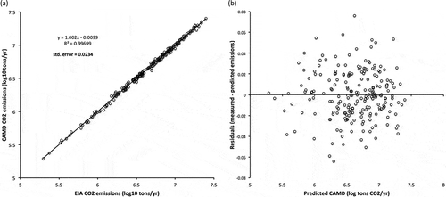
Quick (2014) argues that a transformation was needed because regression of the CO₂ emission amount from one data set on the other results in heteroscedastic regression residuals. Although it is questionable whether or not a linear regression model (which assumes a predictor/response relationship) is the correct form of analysis for these two independent measures, transformation by the gross electricity generation from one data set is certainly a poor choice. To demonstrate this, we utilize a physically neutral log transformation instead, which solves the problem of ill-behaved residuals, leaving one with homoscedastic residuals (see Figure 1).

Figure 1. (a) Annual log-transformed EIA and CAMD CO₂ emissions for 210 U.S. power plants. (b) Regression residuals showing a homoscedastic distribution.

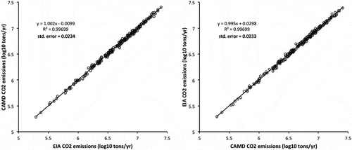
Furthermore, were one to assert that a linear regression with reversed axes supports an attenuation bias (which, as mentioned above, we do not believe is correct), the log transformation we have used as an alternative would lead to the conclusion of no attenuation bias; both the slope coefficient (1.002 vs. 0.995) and its standard error (0.0234 vs. 0.0233) are nearly identical in both cases (see Figure 2). Hence, we consider the test used by Quick (2014) and the conclusion, derived thereof, to be erroneous.

Figure 2. Regression of log-transformed CAMD CO₂ emissions against log-transformed EIA CO₂ emissions (cf. Quick, 2014, figure 3).

An additional argument that utilizes the CO₂ emissions data as a guide to which data set has greater measurement error is found in the Quick (2014) supporting information. The author writes:

Finally, it is useful to simultaneously consider plots where the CAMD and EIA emission rates are used to predict the percent difference between the EIA and CAMD emission rates. These plots are shown by Figure 5S, which shows that the differences between CAMD and EIA emission rates for individual plants are correlated with the CAMD measurement but not with the EIA measurements.

However, the behavior shown on the two panels of figure 5S in Quick (2014) demonstrate no more than what would be expected from comparing two data sets with the same mean but a different level of variation about that mean.

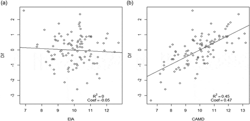
To demonstrate this dynamic, we construct two data sets (virtual EIA emission rate— EIA^v and virtual CAMD emission rate—CAMD^v) that have the same mean value but different levels of variation about that mean. This is accomplished by adding random increments drawn from a distribution with a zero mean and standard deviation of 0.1 to each individual EIA^v value. Thus, we create the CAMD^v data set with the same mean but a larger variance. As in Quick (2014), the difference is regressed against each individually (Figure 3). The relative difference shows no correlation to the EIA^v data set but exhibits correlation to the CAMD^v.

Figure 3. The relationship between the relative difference and the (a) virtual EIA data set (EIA^v) and (b) the virtual CAMD data set (CAMD^v), constructed by adding incremental values to each EIA^v datum with zero mean and standard deviation of 1.

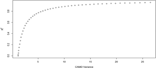
Multiple sets of these paired data sets are constructed by increasing the standard deviation (0.2, 0.3, 0.4, etc.) of the distribution from which the incremental values are drawn. The relative difference is calculated and correlated to both the original EIA^v and CAMD^v. The correlation values for the relative difference to the CAMD^v values are a direct function of the level of variance added (Figure 4).

Figure 4. The relationship between the level of increment variance added to the virtual CAMD data set (x-axis) and the correlation value (y-axis).

As with the central argument in figure 3 of the Quick (2014) main text, the results only demonstrate that one data set has more variation than the other. However, none of the analysis indicates that the greater variation is reflective of the physical reality at these power plants. In short, the smaller variance in the EIA estimates does not necessarily indicate less error.

After arriving at the conclusion that the EIA CO₂ emissions estimates were more accurate than the CAMD estimates, the balance of the Quick (2014) paper provides useful insight into candidates of uncertainty for both the EIA and CAMD data. Although a number of potential uncertainty sources are described, and the nominal uncertainties itemized, there are no independent data to test whether or not these nominal uncertainties are in fact achieved. Hence, they provide no additional support for the contention that one data set is more accurate than the other.

References

- Hutcheon, J.A., A. Chiolero, and J.A. Hanley. 2010. Random measurement error and regression dilution bias. BMJ 340:1402–1406. doi:10.1136/bmj.c2289
- Quick, J.C. 2014. Carbon dioxide emission tallies for 210 U.S. coal-fired power plants: A comparison of two accounting methods. J. Air Waste Manage. Assoc. 64:73–79. doi:10.1080/10962247.2013.833146
- U.S. Environmental Protection Agency. 2014a. Inventory of U.S. Greenhouse Gas Emissions and Sinks: 1990–2012. EPA 430-R-14-003. Washington, DC: U.S. Environmental Protection Agency, April 15, 2014.
- U.S. Environmental Protection Agency. 2014b. Carbon Pollution Emission Guidelines for Existing Stationary Sources: Electric Utility Generating Units; 40 CFR Part 60. Washington, DC: U.S. Environmental Protection Agency, June 2, 2014.