A self-consistent method to assess air quality co-benefits from U.S. climate policies

Abstract

Air quality co-benefits can potentially reduce the costs of greenhouse gas mitigation. However, whereas many studies of the cost of greenhouse gas mitigation model the macroeconomic welfare impacts of mitigation, most studies of air quality co-benefits do not. We employ a U.S. computable general equilibrium economic model previously linked to an air quality modeling system and enhance it to represent the economy-wide welfare impacts of fine particulate matter. We present a first application of this method to explore the efficiency and distributional implications of a Clean Energy Standard (CES) and a Cap and Trade (CAT) program that both reduce CO₂ emissions by 10% in 2030 relative to 2006. We find that co-benefits from fine particulate matter reduction (median $6; $2 to $10/tCO₂) completely offset policy costs by 110% (40% to 190%), transforming the net welfare impact of the CAT into a gain of $1 (−$5 to $7) billion 2005$. For the CES, the corresponding co-benefit (median $8; $3 to $14/tCO₂) is a smaller fraction (median 5%; 2% to 9%) of its higher policy cost. The eastern United States garners 78% and 71% of co-benefits for the CES and CAT, respectively. By representing the effects of pollution-related morbidities and mortalities as an impact to labor and the demand for health services, we find that the welfare impact per unit of reduced pollution varies by region. These interregional differences can enhance the preference of some regions, such as Texas, for a CAT over a CES, or switch the calculation of which policy yields higher co-benefits, compared with an approach that uses one valuation for all regions. This framework could be applied to quantify consistent air quality impacts of other pricing instruments, subnational trading programs, or green tax swaps.

Implications: Policies that reduce CO₂ emissions can also reduce PM_2.5 (particulate matter with an aerodynamic diameter <2.5 μm), yielding unintended economic benefits. Using an integrated assessment model linking policies and emissions to a consistent treatment of costs and co-benefits, we find that PM_2.5 co-benefits offset the costs of reducing CO₂ through Cap and Trade (CAT) in the United States. An equivalent Clean Energy Standard is more costly, and its higher PM_2.5 reductions offset up to a tenth of its costs. Most co-benefits accrue to eastern states, and interregional differences and indirect economic effects shift those gains further to New York and New England. Economy-wide co-benefits reduce the costs and shift the distributional impacts of U.S. carbon policies.

Introduction

Policies for cutting CO₂ emissions to mitigate climate change can improve regional air quality by incidentally reducing polluting activities. These air quality improvements can have welfare co-benefits (or ancillary benefits) that help to compensate for the cost of carbon policies. A growing body of literature has quantified the air quality co-benefits of carbon policy, in part to help identify policies that benefit air quality and climate simultaneously. However, studies of air quality co-benefits often use different methods to assess costs and benefits, precluding direct cost-benefit comparisons. Here, we develop a consistent approach to assess costs and economy-wide air quality co-benefits, by extending and applying an economic model developed to estimate emission changes and policy costs of U.S. climate policies. Specifically, we implement an approach to model and quantify the economy-wide welfare implications of air pollution reductions and compare these air quality impacts with the costs of two U.S. carbon policies.

There is mounting evidence that air quality co-benefits significantly offset the costs of greenhouse gas mitigation (Muller, 2012; Jack and Kinney, 2010; Ravishankara et al., 2012). Nemet et al. (2010) summarize 37 peer-reviewed studies that estimate the air quality co-benefits of climate change policy, with results ranging from $2 to $147/tCO₂. Many assessments of the co-benefits of climate policies use partial equilibrium or computable general equilibrium (CGE) economic models to estimate the costs of climate policies (Nemet et al., 2010; Bell et al., 2011; Burtraw et al., 2003). CGE models use general equilibrium theory to assess the long-run dynamics of resource allocation and income distribution in market economies. They have been widely applied since the early 1990s to evaluate the efficiency of environmental and energy policy (Bergman, 2005), including studies to estimate the cost of the U.S. Clean Air Act and the Acid Rain Trading program (Hazilla and Kopp, 1990; Goulder et al., 1997). By simulating the entire economy, CGE models offer the advantage of estimating changes to emissions from all sectors, including nonregulated sectors that respond to changing prices (Scheraga and Leary, 1994). Accounting for relative price changes throughout the economy is particularly important when projecting substantial climate or energy policy (Sue Wing, 2009; Bhattacharyya, 1996).

In contrast to the well-developed literature on the macroeconomic costs of climate policies, studies estimating air quality benefits use more varied methodologies, most of which do not capture macroeconomic effects. Early studies of the air quality co-benefits of climate policy quantified benefits by applying linearized $/ton estimates of avoided damages from pollutant emissions (Goulder, 1993; Scheraga and Leary, 1994; Boyd et al., 1995). Later studies applied more detailed emissions-impact relationships, including information from source-receptor atmospheric modeling and updated information on concentration-response functions and associated costs (Burtraw et al., 2003; Holmes et al., 1995; Dowlatabadi et al., 1993; Rowe et al., 1995). Health damages are most often valued using estimates of the willingness-to-pay (WTP) for reduced health risks (Bell et al., 2011). WTP estimates for reduced mortality risk, termed Value of a Statistical Life (VSL), constitute the majority of these benefits estimates (Office of Information and Regulatory Affairs [OIRA], 2013). Macroeconomic CGE analysis attempts to incorporate and build on this approach by including the constraints of multiple policies, limited resources, and changing prices, which can lead to significant indirect gains or losses (Smith and Carbone, 2007). Since top-down economic modeling approaches such as CGE are commonly applied to estimate the costs of climate policy (Paltsev and Capros, 2014), a consistent assessment of the air quality co-benefits would use a similar approach to capture indirect gains as well as indirect losses.

A growing number of studies have used CGE models to estimate the macroeconomic and welfare impacts of air pollution. These studies link the human health impacts from fine particulate matter and ozone to welfare loss through increased medical expenses, lost wages, pain and suffering, and reductions in the supply of labor. CGE models have been used to evaluate benefits from the U.S. Clean Air Act (CAA) from 1975 to 2000 (Matus et al., 2008), global ozone impacts under future climate and mitigation scenarios (Selin et al., 2009), and the historical burden of air pollution in Europe (Nam et al., 2010) and China (Matus et al., 2012); however, none of these studies assessed policy costs. The EPA’s Second Prospective Analysis of the CAA evaluated both human health benefits and costs using a CGE framework, but it used pollution changes generated outside the CGE model (EPA, 2011). The studies discussed above have used CGE models to estimate either the cost of environmental policy or the benefits of air pollution reductions, but not both.

Here, we present a method for the consistent evaluation of costs and co-benefits of carbon policies. We present an approach to quantify the economy-wide welfare impacts of air pollution reductions in the same macroeconomic model used to assess emission changes and policy costs. We adapt a multiregion, multisector, multihousehold CGE model of the U.S. economy, the U.S. Regional Energy Policy Model (USREP). This model was previously linked with a detailed emission inventory and air quality modeling system (Thompson et al., 2014a) to estimate policy costs, emission changes, pollution changes, and human health impacts. We present a first application of this method to a national Clean Energy Standard and an equivalent Cap and Trade program. We compare the economy-wide labor and health impacts from fine particulate matter reductions that arise incidentally from each policy. We explore how these co-benefits affect both the efficiency (by reducing policy costs) and the distributional implications of each policy, by modeling how net co-benefits of a national policy are distributed across the continental United States. With our more consistent co-benefits, we reexamine the question: Can the impacts of air quality co-benefits on economic resources “pay for” a climate or clean energy policy in the United States?

Integrated Assessment Methods

We use an integrated assessment framework to model policies, emissions, and impacts, shown in Figure 1. The United States Regional Energy Policy (USREP) economic model (Rausch et al., 2010) is used at the beginning and the end of our analysis process. At the beginning, USREP is used to implement climate policies, quantify costs, and estimate emission changes (Rausch et al., 2011). The Comprehensive Air Quality Model with Extensions (CAMx) (Environ International Corporation, 2011) is next used to link emissions to atmospheric concentrations. The Environmental Benefits Mapping and Analysis Program (BenMAP) (Abt Associates Inc., 2012) is used to estimate human health impacts related to fine particulate matter. As the methodological contribution of this paper, we add a final step to the analysis by using BenMAP-derived health impacts to derive estimates of economy-wide co-benefits in USREP.

Figure 1. Integrated assessment framework for estimating air quality co-benefits of U.S. climate policy. This framework first implements policies in our economic model (USREP), then estimates the resulting impacts to welfare, production, and emissions. Emissions in SMOKE are input to the air quality model CAMx to yield concentrations of fine particulate matter. Those concentrations are input to BenMAP to estimate human health impacts. Lastly, those health impacts are input to USREP to estimate the welfare impacts of fine particulate matter pollution.

This section presents the USREP model, its link to our air quality modeling system and health impacts assessment, our extension of the USREP model to include economy-wide air quality co-benefits, and our application of this new integrated approach to a U.S. national Clean Energy Standard and Cap and Trade program.

The U.S. Regional Energy Policy model

We use USREP to analyze two U.S.-wide carbon policies and to estimate their costs, their effects on pollutant emissions, and their respective air quality co-benefits. USREP is a multiregion, multicommodity, multihousehold recursive-dynamic computable general equilibrium (CGE) model of the U.S. economy, whose input and structure are described in detail in Rausch et al. (2010) and Rausch et al. (2011). USREP calculates commodity prices that support equilibrium between supply and demand in all markets based on the microeconomic decisions of rational agents (i.e., it is a classical Arrow-Debreu model). By including rich detail in the energy sector, and by relating production to emissions of greenhouse gases, USREP is designed to explore the long-run dynamics and the economy-wide costs, emission impacts, and distributional implications of both national and subnational energy and climate change policies. USREP has been applied previously to study climate change and energy policies, exploring their effects on economic growth, efficiency, distribution, and interactions with existing distortionary taxes (Rausch et al., 2010, 2011; Caron et al., 2015; Rausch and Mowers, 2014).

USREP assesses equilibrium conditions over 5-yr periods among profit-maximizing firms and utility-maximizing consumers that receive income from supplying four factors of production (labor, capital, land, and resources). USREP is a full employment model, with the labor supply determined by the household choice between labor and leisure. Taxes are collected by the government and spent on consumption and transfers to households (Rausch et al., 2010).

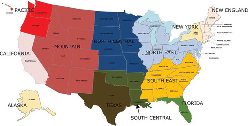
As shown in Table 1, USREP contains 12 geographic regions, 9 household income groups, 5 energy commodities, 5 nonenergy sectors, and advanced “backstop” energy technologies (e.g., advanced solar energy is a “backstop” for fossil energy, as it can produce a close substitute for this nonrenewable resource). Production is characterized by nested constant-elasticity-of-substitution (CES) functions, the details of which are in Rausch et al. (2010). The geographic regions include California, Texas, and Florida, and several multistate composites, shown in Figure 2.

Table 1. USREP model details: Regional, household, and sectoral breakdown and primary input factors

Sectors	Regions	Primary Production Factors	Household Income Classes ($1,000 of annual income)
Nonenergy	Pacific (PACIF)	Capital	<10
Agriculture (AGR)	California (CA)	Labor	10–15
Services (SRV)	Alaska (AK)	Coal resources	15–25
Energy-intensive products (EIS)	Mountain (MOUNT)	Natural gas resources	25–30
Other industries products (OTH)	North Central (NCENT)	Crude oil resources	30–50
Commercial transportation (TRN)	Texas (TX)	Hydro resources	50–75
Passenger vehicle transportation (TRN)	South Central (SCENT)	Nuclear resources	75–100
Final demand sectors	North East (NEAS)	Land	100–150
Household demand	South East (SEAST)	Wind	>150
Government demand	Florida (FL)
Investment demand	New York (NY)
Energy	New England (NENGL)
Coal (COL)
Natural gas (GAS)
Crude oil (CRU)
Refined oil (OIL)
Electric: Fossil (ELE)
Electric: Nuclear (NUC)
Electric: Hydro (HYD)
Advanced technologies

Figure 2. The 12 regions of the USREP model. They are the aggregation of the following states: NEW ENGLAND = Maine, New Hampshire, Vermont, Massachusetts, Connecticut, Rhode Island; SOUTH EAST = Virginia, Kentucky, North Carolina, Tennessee, South Carolina, Georgia, Alabama, Mississippi; NORTH EAST = West Virginia, Delaware, Maryland, Wisconsin, Illinois, Michigan, Indiana, Ohio, Pennsylvania, New Jersey, District of Columbia; SOUTH CENTRAL = Oklahoma, Arkansas, Louisiana; NORTH CENTRAL = Missouri, North Dakota, South Dakota, Nebraska, Kansas, Minnesota, Iowa; MOUNTAIN = Montana, Idaho, Wyoming, Nevada, Utah, Colorado, Arizona, New Mexico; PACIFIC = Oregon, Washington, Hawaii.

The USREP model is based on 2006 state-level economic data from the Impact analysis for PLANning (IMPLAN) data set and energy data from the Energy Information Administration’s State Energy Data System (SEDS). The energy supply is regionalized with data on regional fossil fuel reserves from the U.S. Geological Service and the Department of Energy. Further details on the input data are contained in Rausch and Mowers (2014). Several studies examine the effect of varying model inputs and structure, such as the source of household income data (Rausch et al., 2011) and the structure of the energy system model (Rausch and Mowers, 2014; Lanz and Rausch, 2011). Paltsev and Capros (2014) list numerous studies that have explored the effects on climate mitigation costs of assumptions about innovation, low-carbon technologies, flexibility to substitute energy to low-carbon options, other regulations and regulatory credibility to trigger long-term investment, timing of actions, and the reference scenario.

Linking USREP to emissions and health outcomes

Economic activity was linked to emissions, concentrations, and health outcomes by coupling USREP to an air quality modeling system and health impact model. The details of this approach, including projected pollutant emissions and concentrations under selected carbon policies, are described in full by Thompson et al. (2014a) and summarized below.

Emissions to concentrations

USREP was linked to an air quality modeling system with a national emission inventory for 2005. The inventory was speciated and temporally processed using Spare Matrix Operating Kernel Emissions (SMOKE) (Community Modeling and Analysis System [CMAS], 2010). Production in USREP was linked to the relevant emission sources in the detailed emission inventory by mapping each USREP sector and region to its corresponding sources in the emission inventory. To estimate future emissions in 2030, the relative change in production for each sector and region in USREP was used to scale the corresponding sources in the 2005 emission inventory. For example, an increase in electricity generation from natural gas in USREP caused a proportional increase in all relevant pollutant emissions associated with the production, transportation, and use of natural gas for electricity. All relevant anthropogenic emission sources—including point sources and area sources—were scaled and run through SMOKE to produce gridded, hourly emissions for each scenario.

Projected 2030 emissions were used to estimate future hourly fine particulate matter concentrations on a 36-km grid of the continental United States using the Comprehensive Air Quality Model with Extensions (CAMx) version 5.3 (Environ International Corporation, 2011). To isolate the effects of policy efforts on the emissions of fine particulate matter and its precursors, we did not incorporate climate change in our analysis; emissions are expected to exceed the effect of climate change on U.S. fine particulate matter in 2030 (Penrod et al., 2014). Instead, meteorological input for the year 2005 was used for both present and future simulations, and was developed with the fifth-generation Penn State/National Center for Atmospheric Research (NCAR) mesoscale model MM5 (Grell et al., 1994). CAMx has been used in numerous evaluations of U.S. air quality policy (EPA, 2011, 2012). The year-long air quality modeling episode for 2005 that we use as our base year was developed as part of a base case to evaluate the proposed Cross-State Air Pollution Rule, which was documented and evaluated in EPA (2011).

Concentrations to health outcomes

We calculate mortality and morbidity resulting from fine particulate matter concentrations using the Environmental Benefits Mapping and Analysis Program (BenMAP) version 4.0. Previous studies using this air pollution episode analyzed benefits of both ozone and fine particulate matter reductions (Thompson et al., 2013, 2014a, 2014b). Here, we focus on fine particulate matter, estimating both morbidity and mortality following the methods used in the Regulatory Impact Assessment (RIA) for the fine particulate matter National Ambient Air Quality Standard (EPA, 2012). Table 2 lists the endpoints and concentration-response functions applied. Following the RIA’s approach, we have estimated the lower and upper bounds of the number of health impacts based on both the selection of health impact functions and the uncertainty in those functions, as specified in Table 2.

Table 2. Endpoints, epidemiologic studies, and valuations used for fine particulate matter health impacts, following EPA (2012)

Endpoint/Endpoint Group		Ages (yr)	Individual Studies	Pooling and Lower/Upper Bounds	Valuation 2006$
Premature mortality		>30	Krewski et al. (2009) and Lepeule et al. (2012)	Upper bound: Lepeule (2012) 95th percentile	N/A
				Lower bound: Krewski et al. (2009) 5th percentile
Nonfatal myocardial infarction			Peters et al. (2001), Pope et al. (2006), Sullivan et al. (2005), Zanobetti et al. (2009), Zanobetti and Schwartz (2006)	Upper bound: Peters et al. (2001) 95th percentile	$100,000
				Lower bound: 5th percentile of equal-weights pooling of 4 other studies
Respiratory hospital admissions	All	>64	Zanobetti et al. (2009)—ICD 460-519 (All respiratory)	Pooling of: All respiratory: Pooling of Zanobetti et al. (2009) and Kloog et al. (2012)	$23,711
			Kloog et al. (2012)—ICD 460–519 (All respiratory)
	COPD	18–64	Moolgavkar (2000)—ICD 490–492, 494–496 (COPD, less asthma)	Asthma: Pooling Babin et al. (2007) and Sheppard (2003)	$15,903
	Asthma	<18	Babin et al. (2007)—ICD 493 (asthma), Sheppard (2003)—ICD 493 (asthma)	COPD (less asthma): Moolgavkar (2000)	$10,040
Cardiovascular hospital admissions		>64	Zanobetti et al. (2009)—ICD 390–459 (all cardiovascular)	Pooling of all 4 studies for ages >64 added to Moolgavkar (2000) for ages 18–64	$27,319
			Peng et al. (2009)—ICD 426–427; 428; 430–438; 410–414; 429; 440–449 (Cardio-, cerebro-, and peripheral vascular disease)
			Peng et al. (2008)—ICD 426–427; 428; 430–438; 410–414; 429; 440–449 (Cardio-, cerebro-, and peripheral vascular disease)
			Bell et al. (2008)—ICD 426–427; 428; 430–438; 410–414; 429; 440–449 (Cardio-, cerebro-, and peripheral vascular disease)
		18–64	Moolgavkar (2000)—ICD 390–429 (all cardiovascular)		$29,364
Asthma-related ER visits		<18	Mar et al. (2010), Slaughter et al. (2005), Glad et al. (2012)	Pooling of all 3 studies	$370
Acute bronchitis		8–12	Dockery et al. (1996)	N/A	$416
Lower respiratory symptoms		7–14	Schwartz and Neas (2000)	N/A	$18
Upper respiratory symptoms		9–11	Pope et al. (1991)	N/A	$29
Asthma exacerbation		6–18	Ostro et al. (2001) (cough, wheeze, shortness of breath), Mar et al. (2004) (cough, shortness of breath)	Pooling of Ostro et al. (2001) and Mar et al. (2004)	$50
Minor restricted-activity days		18–64	Ostro and Rothschild (1989)	N/A	$60
Work loss days		18–64	Ostro (1987)	N/A	$150

Notes: ER = emergency room; ICD = International Statistical Classification of Disease; COPD = chronic obstructive pulmonary disease.

Economic modeling of air quality co-benefits

For this study, we incorporate the economic and welfare effects of pollution-related health outcomes into USREP, accounting for morbidities and mortalities with separate techniques. Our focus is on the change in consumer welfare, which can be generally understood as the income amount that would be necessary to compensate consumers for losses under a policy. Our welfare index includes the change in macroeconomic consumption (capturing market-based activities) and the change in leisure (i.e., the monetary value of the change in nonworking time) in response to policy (Paltsev and Capros, 2014). We account for morbidities through lost wages, lost leisure, and medical expenses that vary with pollution levels. We account for mortality by reducing the supply of labor accordingly.

Morbidities in USREP

We account for morbidities related to fine particulate matter by representing the change in medical expenditures and lost wages through a new sector added to USREP. We add a household production sector for “pollution health services” whose production is determined by the pollution level and the valuation of the resulting health outcomes. The valuation of each morbidity endpoint is shown in Table 2, following EPA (2012). These valuations are derived from estimates of willingness-to-pay (i.e., for asthma exacerbation and upper respiratory symptoms), medical costs, and lost wages, using U.S. data. Similar approaches incorporate willingness-to-pay in CGE models to estimate air quality impacts, representing nonmarket losses as lost leisure (Matus et al., 2008; Selin et al., 2009; Nam et al., 2010; Matus et al., 2012). Smith and Carbone (2007) discuss the theoretically preferred approach and remaining empirical challenges to incorporating air quality preferences in CGE models. We follow EPA (2012) because these valuations are based on U.S. data and studies and have been applied in evaluating U.S. air quality regulations (EPA, 2011, 2012). Within USREP, we apply the valuation per case to the number of cases estimated using BenMAP and use the total valuation to calculate the demand for resources for the new “pollution health services” sector.

The “pollution health services” sector tracks the demand for economic resources in response to pollution-related health outcomes. Higher pollution reduces welfare by requiring more resources per health outcome. Each outcome creates economic impacts composed of medical costs, lost labor, and other disutility (e.g., pain and suffering). We map these impacts to demand for sectoral inputs of services and labor using functions for each endpoint developed by Yang (2004) and Matus et al. (2008). The fine particulate matter pollution levels affect the output of the pollution health services sector, with higher pollution drawing more resources per unit of output (termed a Hicks neutral negative technical change). Policies that reduce pollution increase welfare, as lower pollution increases the productivity of this sector.

We add this new sector to those listed in Table 1, following Matus et al. (2008) and Nam et al. (2010). It requires inputs of service, which are drawn from the services (“SRV”) sector, and of labor, which are drawn from the household labor supply. The output of this new sector is included in private consumption. It thus forms a component of household welfare, i.e., the sum of consumption and leisure.

Mortalities in USREP

We do not value pollution-related mortalities directly (e.g., with a VSL estimate), but instead estimate how they affect welfare by reducing the supply of labor. Higher pollution-related mortality reduces welfare in a region by reducing the supply of labor, thereby increasing production costs and decreasing consumption. We first estimate the change in the adult (>30 yr) population by dynamically reducing the census-based population projections in USREP by the amount of pollution-related mortalities from BenMAP. We apply a 2/3 labor participation rate of adults (i.e., the employment-to-population ratio) to estimate the percent change in the labor force from the percent change in population, as in Matus et al. (2008). We apply the change in labor force to the year in which the death took place, effectively accounting for 1 yr of life lost per death. Estimating the actual years of life lost would increase our estimates of the labor impact of mortality. By reducing the labor supply, we affect wage rates, which in turn affect workers’ decisions on how to use their total time endowment, represented in USREP as a substitution between labor and leisure (Rausch et al., 2010).

Climate change policies

Clean Energy Standard and equivalent Cap and Trade program

We apply our modeling framework to estimate economy-wide co-benefits from fine particulate matter reductions under two national climate policies, previously implemented in USREP (Rausch and Mowers, 2014). These policies’ air quality implications and estimated co-benefits were previously assessed by applying VSL measures to mortalities from fine particulate matter and ozone (Thompson et al., 2014a).

Our first policy is a Clean Energy Standard (CES) similar to the proposed Clean Energy Standard Act of 2012 (Bingaman et al., 2012). This policy doubles clean energy from 42% to 80% by 2035, beginning in 2012, by setting specified percentages of electricity sales from qualified energy sources. The second policy is an equivalent U.S. economy-wide Cap and Trade program (CAT). The revenue from auctioned emissions permits for the CAT is returned lump sum to households on a per capita basis (Rausch and Mowers, 2014). Both policies reduce equivalent CO₂ emissions, i.e., 500 million metric tons CO₂, or a 10% reduction in 2030 relative to 2006 emissions. Both the CAT and CES are compared with a Business As Usual (BAU) scenario in which CO₂ emissions grow to 6200 mmt by 2030. We analyze these policies as they were implemented in USREP by Thompson et al. (2014a). We estimate the costs of each policy as the cumulative, undiscounted change in welfare (i.e., material consumption and leisure) for all regions from 2006 to 2030 compared with BAU.

Estimating welfare impacts of policies from fine particulate matter reductions over time

To estimate co-benefits from fine particulate matter reductions, we first average our CAMx output to the temporal and spatial scales of USREP. From CAMx we obtain daily concentrations in 2005 as well as in 2030 for our BAU, CAT, and CES scenarios. We combine those concentrations with census data to obtain population-weighted annual average concentrations for each USREP region contained in our air quality modeling grid. Because we model air quality in the continental United States only, we do not estimate co-benefits for Alaska and Hawaii.

To capture cumulative impacts as reductions are gradually realized, we interpolate pollution reductions between 2005 and 2030 and their health effects over our analysis period of 2006–2030. For morbidities, that pollution change (in every 5-yr period and region) becomes the (Hicks neutral) negative scaling factor that affects the productivity of the health services sector. Under BAU, we assume population-weighted pollution levels follow a linear progression from 2006 to 2030 levels. Our policies begin implementation in 2012. We assume pollution levels follow BAU from 2006 to 2012, and then assume a linear implementation of the remaining reductions from 2012 to 2030 for each policy. For mortalities, we estimate total deaths from the change in fine particulate matter between 2006 and 2030 in BenMAP for BAU and both policies. We then follow the same interpolation process for mortalities as for the pollution levels to allocate those deaths over the periods in BenMAP between 2006 and 2030. Over time, increases in labor productivity and population size and age each serve to increase the value of a policy’s pollution reductions compared with BAU.

To estimate economy-wide co-benefits, we run USREP six more times from 2006 to 2030. We run USREP twice for each of the three scenarios, BAU, CES, and CAT, using the corresponding pollution levels and the lower and upper bounds of the health effects estimates, respectively. The upper and lower bounds are determined following EPA (2012) and are based on the 95% confidence intervals of individual or pooled studies in combination with the selection of different studies to assess the lower and upper bounds of outcomes for each endpoint. We estimate the co-benefits of each policy as the cumulative, undiscounted change in welfare (i.e., material consumption and leisure) compared with BAU. This change in welfare is our estimate of each policy’s air quality co-benefit.

Integrated assessment process: Policy costs to air quality co-benefits in one framework

To summarize this process, depicted in Figure 1, results from USREP are used to estimate the policy costs and economic activity under BAU, CAT, and CES, respectively. Those economic activities were mapped to emissions of particulate matter and its precursors in 2030 by scaling a detailed emission inventory for 2005 in SMOKE, and fine particulate matter concentrations in 2005 and 2030 were estimated by CAMx (Thompson et al., 2014a). Based on these previous results, we create upper and lower bound estimates of morbidities and mortalities over time with BenMAP. We then run USREP again to estimate the lower and upper bounds of air quality welfare impacts for each of BAU, CES, and CAT. Thus, we use the economy-wide impacts of complying with each policy to model future pollutant concentrations and their economy-wide impacts due to human health responses. We estimate net co-benefits by subtracting air quality co-benefits from the policy cost.

Results: Co-benefits from Fine Particulate Matter Reductions

We present estimates of air quality co-benefits for each policy, on a total, a per capita, and a per ton of CO₂ basis. We then sum the welfare impacts of pollution and policy implementation to calculate net co-benefits. We compare co-benefits with costs to estimate the fraction by which co-benefits reduce policy costs. We present results at the national scale followed by the regional scale. Finally, we explore how general equilibrium and cumulative effects contribute to our results, both in terms of policy efficiency (i.e., net co-benefits) and distributional implications. Intermediate results describing changes in emissions, mortalities, and health outcomes are provided in Supplemental Material.

National air quality co-benefits and net co-benefits by policy

National co-benefits

Co-benefits from fine particulate matter reductions for each policy compared with BAU are presented in Table 3. We show the median and the upper and lower bounds derived from the uncertainty in the health estimates, as in Table 2. All values are denominated in constant year 2005 U.S. dollars (i.e., 2005$). Nationally, we estimate that the CES yields higher co-benefits ($13 billion, with a range of $4 to $21 billion) than the CAT program ($9 billion; range $3 to $15 billion), measured as cumulative benefits by 2030 in 2005$. This reflects the greater fine particulate matter reductions under the CES than under the CAT (reduction in population-weighted annual average daily mean of 0.97 µg m⁻³ for CES, compared with 0.56 µg m⁻³ for CAT) (Thompson et al., 2014a). These co-benefits correspond to $8 ($3 to $14)/tCO₂ for the CES, and $6 ($2 to $10)/tCO₂ for the CAT.

Table 3. Median co-benefits of each policy (total, per capita, and per ton of mitigated CO₂ emissions) [range in square brackets]

	Co-benefits (million 2005$)		Co-benefits Per Capita (2005$)		Co-benefits Per Ton of CO2 Mitigated (2005$/tCO2)
Region	CES	CAT	CES	CAT	CES	CAT
National	$12,800	$8,700	$35	$24	$8	$6
	[$4,500, $21,000]	[$2,800, $14,600]	[$12, $57]	[$8, $40]	[$3, $14]	[$2, $10]
West	$2,800	$2,500	$100	$81	$4.1	$29
	[$900, $4,600]	[$630, $4,370]	[$40, $150]	[$22, $140]	[$1.2, $7.0]	[$7, $51]
East	$10,000	$6,200	$260	$190	$140	$40
	[$3,500, $17,000]	[$2,200, $10,200]	[$90, $430]	[$70, $320]	[$40, $240]	[$10, $60]
Pacific	$81	$55	$5	$4	$2	$4
	[$81, $81]	[$19, $90]	[$5, $5]	[$1, $6]	[$1, $4]	[$1, $6]
California	$270	$440	$6	$9	$4	$10
	[$80, $450]	[$70, $810]	[$2, $10]	[$2, $17]	[$1, $6]	[$2, $19]
Mountain	$200	$260	$7	$9	$1	$1.5
	[$60, $340]	[$40, $490]	[$2, $11]	[$1, $16]	[$0, $2]	[$0.2, $2.7]
North Central	$980	$460	$45	$21	$6*	$4
	[$400, $1,600]	[$190, $730]	[$18, $71]	[$9, $33]	[$2, $9]	[$1, $6]
Texas	$1,100	$1,280	$32	$38	$4	$10
	[$300, $1,800]	[$310, $2,250]	[$10, $55]	[$9, $68]	[$1, $7]	[$2, $18]
North East	$3,900	$2,200	$48	$26	$11	$9
	[$1,400, $6,400]	[$800, $3,500]	[$17, $79]	[$9, $44]	[$4, $19]	[$3, $14]
New England	$560	$1,000	$36	$66	$98	$7
	[$140, $980]	[$400, $1,700]	[$9, $63]	[$24, $109]	[$24, $170]	[$2, $11]
New York	$680	$660	$35	$34	$10	$7
	[$240, $1,100]	[$260, $1,050]	[$12, $58]	[$13, $54]	[$3, $16]	[$3, $11]
South Central	$660	$280	$55	$24	$6	$3
	[$290, $1,000]	[$100, $470]	[$24, $87]	[$8, $39]	[$2, $9]	[$1, $5]
South East	$3,400	$1,700	$57	$28	$8	$7
	[$1,100, $5,600]	[$600, $2,700]	[$19, $95]	[$10, $46]	[$3, $14]	[$3, $12]
Florida	$840	$440	$29	$15	$7	$2
	[$340, $1,300]	[$120, $750]	[$12, $47]	[$4, $26]	[$3, $12]	[$1, $4]

Notes: The CES has higher co-benefits than the CAT, nationally and across regions. Co-benefits from fine particulate matter reductions by each policy are expressed in terms of (1) the cumulative, undiscounted change in welfare (i.e., material consumption and leisure) compared with BAU from 2006 to 2030 (million 2005$); (2) the equivalent welfare change per capita (2005$); (3) the welfare change per ton of CO₂ mitigated. The median appears along with the range estimated from the uncertainty in health estimates in square brackets. Negative values are in round brackets. West and East are divided by the Mississippi River, and their values are the sums of their respective regions. *In the North Central region, CO₂ emissions actually rise slightly (by 5%) under the CES due to increased coal and gas use in the electricity sector.

National net co-benefits

We compare the air quality co-benefits of each policy with its respective cost, reported as the cumulative, undiscounted change in welfare (i.e., material consumption and leisure) compared with BAU, shown in Table 4. We calculate net co-benefits as the sum of the modeled welfare changes due to fine particulate matter reductions (always positive) and due to policy implementation (usually negative). Co-benefits are the change in welfare from fine particulate matter changes. Policy costs are the change in welfare from policy implementation; policies can impart welfare gains to some regions, which we term a “positive cost.” Positive net co-benefits indicate a net welfare gain when air quality co-benefits are included in policy costs. The CES is the more expensive policy, costing $242 billion (2005$) compared with $8 billion (2005$) for a CAT that reduces the same amount of CO₂.

Table 4. Co-benefits, costs, and net co-benefits in billions 2005$

	Co-benefit (billion 2005$)		Cost (billion 2005$)		Net Co-benefit (billion 2005$)
Region	CES	CAT	CES	CAT	CES	CAT
National	$13	$9	($242)	($8)	($229)	$1
	[$5, $21]	[$3, $15]			[($237), ($221)]	[($5), $7]
West	$2.8	$3	($92)	($8.2)	($89)	($5.7)
	[$0.9, $4.6]	[$0.6, $4]			[($91), ($87)]	[($7.6), ($3.8)]
East	$10	$6	($150)	$0.4	($140)	$6.7
	[$3.5, $16.5]	[$2, $10]			[($146), ($133)]	[$2.7, $10.7]
Pacific	$0.25	$0.05	$3.2	$0.5	$3	$0.6
	[$0.08, $0.41]	[$0.02, $0.09]			[$3, $4]	[$0.5, $0.6]
California	$0.27	$0.44	($25)	$1.4	($24)	$1.8
	[$0.08, $0.45]	[$0.07, $0.09]			[($25), ($24)]	[$1.4, $2.2]
Mountain	$0.20	$0.26	($17)	($2.5)	($17)	($2.2)
	[$0.06, $0.34]	[$0.04, $0.49]			[($17), ($17)]	[($2.4), ($2.0)]
North Central	$0.98	$0.46	($22)	($2.2)	($21)	($1.7)
	[$0.40, $1.6]	[$0.19, $0.73]			[($21), ($20)]	[($2.0), ($1.5)]
Texas	$1.1	$1.28	($31)	($5.4)	($30)	($4.1)
	[$0.3, $1.8]	[$0.31, $2.25]			[($31), ($29)]	[($5.1), ($3.2)]
North East	$3.9	$2.2	($60)	($1.5)	($56)	$0.7
	[$1.4, $6.4]	[$0.8, $3.5]			[($59), ($54)]	[($0.7), $2.1]
New England	$0.6	$1.0	($6.5)	$2.5	($6.0)	$3.5
	[$0.1, $1.0]	[$0.4, $1.7]			[($6.4), ($5.6)]	[$2.8, $4.2]
New York	$0.7	$0.7	($6.9)	$0.3	($6.2)	$1.0
	[$0.2, $1.1]	[$0.3, $1.1]			[($6.7), ($5.8)]	[$0.6, $1.4]
South Central	$0.7	$0.28	($13)	($1.4)	($12)	($1.1)
	[$0.3, $1.0]	[$0.10, $0.47]			[($13), ($12)]	[($1.3), ($0.9)]
South East	$3.4	$1.7	($37)	$0.2	($34)	$1.9
	[$1.1, $5.6]	[$0.6, $2.7]			[($36), ($32)]	[$0.8, $3.0]
Florida	$0.8	$0.4	($26)	$0.3	($25)	$0.7
	[$0.3, $1.3]	[$0.1, $0.7]			[($26), ($25)]	[$0.4, $1.1]

Notes: The CAT is more cost-effective than the CES, and its co-benefits can offset more of its costs, up to 190% (median 110%; 40% to 190%). (1) Co-benefits of each policy are the change in welfare (consumption and leisure) from BAU due to fine particulate matter reductions, expressed in billions 2005$. (2) Costs of each policy are the change (usually a negative change) in welfare (consumption and leisure) from BAU due to the policy implementation, expressed in billions 2005$. Regions that gain from policy implementation (i.e., costs are positive) are highlighted with gray shading. (3) Net co-benefits are the sum of these two welfare changes. Where net co-benefits are positive, cells are emphasized with gray shading. The median appears along with the range estimated from the uncertainty in health estimates. Negative values are in round brackets. West and East are divided by the Mississippi River, and their values are the sums of their respective regions.

We compare co-benefits to policy costs in two ways. We sum co-benefits and policy costs to estimate net co-benefits. Summing co-benefits and costs estimates the amount by which air quality impacts reduce the apparent mitigation costs. If net co-benefits are positive, then fine particulate matter co-benefits completely offset policy costs. Each policy has different costs and co-benefits (e.g., the CES has higher co-benefits and higher costs). Thus, to indicate the relative importance of air quality, we estimate what fraction of policy costs are offset by air quality co-benefits.

We find that the CES has net co-benefits of −$230 (−$237 to −$221) billion 2005$. The CAT has net co-benefits of $1 (−$5 to $7) billion 2005$. This implies that the policy costs of the CES are reduced by 5% (2% to 9%) by ancillary fine particulate matter reductions. For the CAT, up to 190% of the costs are offset by co-benefits (median 110%; 40% to 190%).

Regional air quality co-benefits and net co-benefits by policy

Regional co-benefits

Table 3 shows the distribution of the calculated co-benefits of each policy across the continental United States (total, per capita, and per ton of mitigated CO₂ emissions). Most co-benefits go to regions east of the Mississippi River. For the CES, per capita gains are $260 in 2005$ in the East compared with $95 in the West, with 78% of all gains accruing to eastern regions. For the CAT, 71% of all gains accrue to the East. The distribution of co-benefits is a combination of the pattern of pollution reductions and general equilibrium (GE) economic effects. Because fine particulate matter reductions are greatest in the eastern states under both policies (Thompson et al., 2014a), most co-benefits accrue to those regions. We discuss GE effects in a later results section on the Contribution of General Equilibrium Economic Effects.

Some regions experience high or low co-benefits on a per ton basis. This pattern is the distributional effect of a national policy. To understand the effects of a regional policy, a separate analysis would be required. For example, under the CES, in one region—North Central—CO₂ emissions actually rise by 5%. Thus, the co-benefits per ton of CO₂ in North Central (median $6; range $2 to $9/tCO₂; 2005$) are actually expressed with respect to an increase in CO₂ emissions. CO₂ emissions rise under the CES in North Central due to increased coal and gas use in the electricity sector. This outcome is only possible because compliance with the CES is counted on a national basis and not for each region: if each region had to meet the Clean Energy Standard on its own, this effect would not occur. Similarly, New England only reduces a small amount of CO₂ under the CES, because more cost-effective reductions are realized elsewhere. At the same time, New England still benefits from upwind pollutant reductions and, consequently, appears to have high benefits per ton of $98 ($24 to $170)/tCO₂. As with North Central, if New England had to meet a regional CES of its own, its co-benefits per ton would likely drop as its required CO₂ reductions would rise. If New England unilaterally adopted a CES, its local pollutant emissions might decrease, but its transport of pollution from unconstrained upwind regions might rise compared with a national CES. Given these interregional interactions, the costs and co-benefits in a given region do not depend only on the local impacts of policy or pollution.

Regional net air quality co-benefits

Table 4 displays the co-benefits, the costs, and the net co-benefits by policy and region. The costs are defined as the cumulative change in welfare (consumption and leisure) resulting from compliance with each policy, expressed in billions 2005$. Since “costs” are defined as a welfare change (usually negative), the regions that benefit from implementing these policies have a positive “cost.” Those regions are highlighted in Table 4. Net co-benefits are the sum of the welfare changes due to fine particulate matter reductions (always positive) and due to policy implementation (usually negative). Regions with positive net co-benefits are also highlighted in Table 4.

Implementing each policy does benefit some regions, i.e., their policy “costs” are actually a welfare gain. For the CAT, this is true of the East, which gains $0.4 billion. Individual regions that gain from the CAT are the coastal regions, excepting the North East, i.e., Pacific, California, New England, New York, South East, and Florida. As explained in Rausch and Mowers (2014), coastal regions appear to gain from the CAT because of how we treat its revenue, which we return to households on a per capita basis. Our per capita allocation of carbon revenue overcompensates people in these populous, largely de-carbonized areas (Rausch and Mowers, 2014). For the CES, it is only the Pacific region that gains a relative advantage and reaps $0.5 billion 2005$ relative to BAU.

In terms of net co-benefits, the CAT favors the East whereas the CES favors the West. For the CAT, the East nets a gain of $6.7 ($2.7 to $11) billion 2005$. The West posts a net loss of −$5.7 (−$7.6 to −$3.8) billion 2005$. For the CES, the East and West post net losses of $140 ($133 to $146) and $89 ($87 to $91) billion 2005$, respectively. Under the CES, the East fares worse than the West because its higher co-benefits ($10 billion in the East versus $3 billion in the West) are countered by even higher costs (−$150 billion in the East versus −$92 billion in the West).

For each policy, some regions receive a net gain. For the CAT, net co-benefits are positive in the coastal regions (which gain from policy implementation, i.e., have positive costs), including the North East (where costs are negative). Median net co-benefits in these regions range from $0.7 billion 2005$ in the North East to $3.5 billion 2005$ in New England. For the CES, median net co-benefits are positive only in the Pacific, at $0.4 billion 2005$. Apart from the North East, the regions with positive net co-benefits are the regions that gain under their respective policy implementations, i.e., the regions with positive costs. Thus, the North East under the CAT is the one instance where a region’s positive co-benefits (median $2.2; $0.8 to $3.5) billion 2005$ offset its negative costs of implementation (−$1.5 billion 2005$).

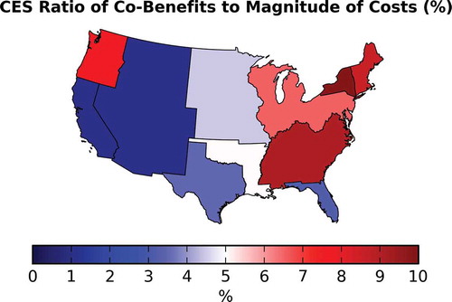
We compare co-benefits of the CES with the magnitude of its policy costs (whether negative or positive) in Figure 3. Everywhere, the welfare impact of implementing a CES is greater than that of the resulting reduction in fine particulate matter. Median CES co-benefits range from 1% (in California) to 10% (in New York) of the magnitude of policy costs. This pattern combines the relative importance of both co-benefits and costs. For example, the Pacific region has a ratio of 8% because its costs are less than in California and Mountain, which have similar co-benefits (co-benefits are Pacific: $0.25, California: $0.26, Mountain: $0.20 billion 2005$) and ratios of 1%. New York and New England similarly reach ratios of 10% and 9% by having the third and second lowest costs. Conversely, the South East has a high ratio compared with other regions because it has the highest co-benefits ($3.4 billion 2005$).

Figure 3. Ratio of median co-benefits to the magnitude of policy costs for the CES (%). Median CES co-benefits range from 1% (in California) to 10% (in New York) of the magnitude of policy costs.

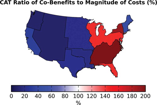
Figure 4 shows the ratios of co-benefits to the magnitude of costs for the CAT, which range from 11% to 690%. Co-benefits exceed the magnitude of policy costs in the East, and in four eastern regions. In the West, they are 0.3 times smaller overall, and range from 11% of costs (in Pacific and Mountain) to 32% in North Central. Co-benefits from pollution reduction in the East are 14 times the welfare impact of compliance. Co-benefits are greater than the magnitude of the cost in Florida, North East, New York, and South East by a factor of 1.4, 1.4, 1.9, and 6.9, respectively.

Figure 4. Ratio of median co-benefits to the magnitude of policy costs for the CAT (%). The relative welfare impact of pollution to policy implementation is greatest in the East, where co-benefits are 14 times greater than costs. Median values are plotted; for the CAT, these range from 11% to 690% and are >100% for Florida, New York, North East, and South East.

Contribution of general equilibrium economic effects

National co-benefits: Contribution of cumulative and indirect effects

In addition to estimating direct morbidity costs, this approach represents cumulative and indirect welfare gains, as fine particulate matter is gradually reduced compared with BAU under each policy. Over the entire 2006–2030 period, the direct effects of morbidities are 9% and 7% of the total co-benefits for the CES and CAT. The remaining 91% and 93% of welfare impacts are the effects of price adjustments and labor productivity (from avoided mortality) that compound over time as they are applied to successively larger populations. This compounding of co-benefits from years prior to 2030 amounts to 42% and 45% of cumulative co-benefits for the CES and CAT, respectively.

Regional co-benefits: Patterns of direct and indirect effects

We compare our distribution of co-benefits with one that values mortalities directly. This comparison illustrates how our approach yields a different regional pattern of co-benefits than would be found using a typical VSL approach. VSL valuations of avoided mortality constitute the majority of fine particulate matter benefits in impact assessments that use them. For example, the Office of Management and Budget’s Office of Information and Regulatory Affairs (OIRA, 2013) cited air quality regulations as having the greatest benefits of all regulations reviewed, and those regulations have >90% of benefits due to VSL valuations of fine particulate matter–related mortality (e.g., EPA, 2012). Thus, the distributional implications of air quality benefits evaluated this way will have a pattern that largely follows the pattern of avoided mortality. Here, we represent mortality as a labor impact, and we also account for the indirect effects of market interactions. Therefore, we expect our distribution of co-benefits to differ from our distribution of avoided mortalities. We explore that difference for each policy.

Under policy, each region avoids a certain number of mortalities, which is a percentage of the total avoided mortalities. Similarly, each region gains a particular share of our estimated co-benefits. Here, we explore the difference in the regional patterns of co-benefits and avoided mortalities by calculating the percentage by which the share of co-benefits differs from the share of avoided mortalities.

If the effect of mortality on welfare were identical in each region, then the difference in these patterns should be zero everywhere. Positive differences would mean that the co-benefits we calculate would be underestimated using one VSL for all regions, whereas negative values mean they would be overestimated.

Morbidities could explain small differences between the shares of co-benefits and mortalities by region. The direct costs of morbidities contribute less than 9% to co-benefits for either policy and are highly spatially correlated with avoided mortalities (97% correlation of avoided morbidities and mortalities by region). Thus, we attribute differences of 10% or more in the share of co-benefits and avoided deaths to differences in the welfare impact of mortality by region, which can arise through differences in relative labor productivity and abundance, and the effects of trade.

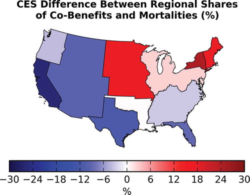
For the CES, the distribution of co-benefits differs from the distribution of mortalities by as much as −25% in California to 25% in New York. Figure 5 shows the percent difference in the share of median co-benefits from the share of median mortalities, cumulative from 2006 to 2030. We find, for example, that New York has 4% of all mortalities avoided by the CES but reaps 5% of the total welfare gain. Thus, the welfare gain from avoided mortalities in New York is greater than in other regions for the CES. The pattern of mortalities is a good predictor of co-benefits, explaining 99% of the variance in co-benefits between regions. However, if we were to apply the national average welfare gain from avoided mortalities to New York, we would underestimate its co-benefits by $132 million 2005$. Conversely, we would overestimate co-benefits in Texas by $138 million 2005$.

Figure 5. Median difference in the share of co-benefits from the share of mortalities (%). For the CES, each region’s share of co-benefits is different than its share of avoided mortalities. Compared with valuing mortality directly with VSL, this approach gives a distributional pattern of co-benefits that differs by as much as −25% in California to 25% in New York.

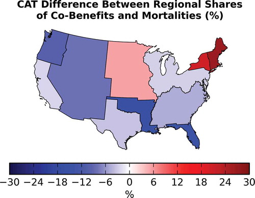
For the CAT, the distribution of co-benefits agrees with the distribution of avoided mortalities within 10% for seven regions, as shown in Figure 6. Using one valuation for mortality risk in all regions would explain over 98% of the variance in co-benefits between regions. It would, however, overestimate co-benefits in every region except North Central, New York, and New England, and would differ in the share of co-benefits by as much as −15% in South Central to 27% in New England. Using the average welfare gain from avoided mortalities would underestimate co-benefits in New York and New England by $100 million 2005$ and $220 million 2005$, respectively.

Figure 6. Median difference in the share of co-benefits from the share of mortalities (%). For seven regions, the pattern of the share of co-benefits matches that of mortalities within 10%. Using one valuation for mortality risk in all regions would overestimate co-benefits in every region except North Central, New York, and New England, and would differ in the share of co-benefits by as much as −15% in South Central to 27% in New England.

Discussion and Conclusion

We present a self-consistent integrated modeling framework to quantify the economy-wide co-benefits of fine particulate matter reductions under climate change and energy policy in the United States. We employ a U.S. economic model previously linked to an air quality modeling system and enhance it to represent the economy-wide welfare impacts of fine particulate matter. We present a first application of this method to explore the efficiency and distributional implications of a Clean Energy Standard and a Cap and Trade program that both reduce CO₂ emissions by 10% in 2030 relative to 2006, including their ancillary impacts to fine particulate matter.

Based on our consistent methodological treatment of both climate policy costs and the co-benefits of air pollution reductions, we find that avoided damages from fine particulate matter alone can completely offset the costs of reducing CO₂ through Cap and Trade in the United States. Up to 190% (median 110%; 40% to 190%) of the CAT’s policy cost are offset by co-benefits of $6 ($2 to $10)/tCO₂ for the CAT. In the process of reducing CO₂ emissions by 10%, the CAT reduces fine particulate matter concentrations by 0.56 µg m⁻³ in 2030 relative to 2006, yielding health-related economic benefits that offset the cumulative welfare impact of the CAT to yield a net impact of $1 (−$5 to $7) billion 2005$.

Although the equivalent Clean Energy Standard yields higher pollution reductions (0.97 µg m⁻³, population-weighted annual average reduction in 2030 versus 2005), the corresponding co-benefit (median $8; $3 to $14/tCO₂) is a smaller fraction (median 5%; 2% to 9%) of its higher policy costs. A less cost-effective means of reducing CO₂ than the CAT, the CES has a net welfare impact (co-benefits minus costs) of −$229 (−$237 to −$221) billion 2005$.

Including air quality co-benefits affects not only the efficiency but also the distributional implications of each policy. The distributional pattern of co-benefits favors the East for both policies, which garners 78% and 71% of gains for the CES and CAT, respectively. On a net co-benefits basis, the CAT favors the East whereas the CES favors the West. The only area with a net gain under either policy is the East, which nets a gain of $6.7 ($2.7 to $10.7) billion 2005$ under the CAT. In several regions in the East under the CAT, the impacts of air quality are greater than the impacts of the policy by a factor of 1.4, 1.4, 1.9, and 6.9 for Florida, North East, New York, and South East, respectively. Overall, co-benefits from pollution reductions in the East are 14 times the welfare impact of compliance with the CAT.

General equilibrium effects shift our distributional implications compared with a traditional analysis that values mortalities directly. Over 90% of our co-benefits arise from a combination of labor and price adjustments as they compound over time, i.e., a combination of the direct labor effects of mortalities with general equilibrium effects. For both policies, avoided mortalities are a good predictor of the co-benefits within a region, but the welfare impact of a healthier labor force differs across regions. General equilibrium effects and interregional differences in labor productivity and supply shift the distribution of our co-benefits compared with the pattern of avoided mortalities. For the CES, the patterns of co-benefits and mortality differ by as much as −25% in California to 25% in New York. For the CAT, the distribution of co-benefits agrees with the distribution of mortalities within 10% for seven regions. However, using a single value for the welfare impact of mortality would overestimate co-benefits in most regions excepting New York and New England, where co-benefits would be understated by $100 million 2005$ and $220 million 2005$, respectively.

We track the economy-wide effect of mortality related to pollution as a reduction in the supply of labor, which yields lower benefits compared with studies that value mortality directly using VSL. Per ton of CO₂ emissions avoided, our co-benefits of $6 ($2 to $10)/tCO₂ for the CAT and $8 ($3 to $14)/tCO₂ for the CES are lower than previous work by Thompson et al. (2014a) and reviewed by Nemet et al. (2010). Thompson et al. (2014a) examined the same policies and particulate matter reductions studied here. They estimated the effects of morbidities and mortalities, which were valued using a VSL approach, yielding $170/tCO₂ for the CAT and $302/tCO₂ for the CES. Our results also fall at the low end of the range of $2 to $196/tCO₂ from 37 studies of air quality co-benefits of climate policy reviewed by Nemet et al. (2010), who note that the higher values of this range derived primarily from developing nations. We attribute this primarily to our treatment of mortality, in addition to our relatively clean setting and moderate policy stringency. In spite of our conservative valuation approach and policy setting, we find that air quality co-benefits can “pay for” 110% (40% to 190%) of the costs of a CAT, indicating the importance of co-benefits even in developed nations.

Our conclusions agree with and complement previous findings on the air quality co-benefits of climate policy. Air quality co-benefits are significant for both climate and energy policies, especially in regions with high pollutant emissions. The CAT policy is the lower-cost option per ton of CO₂ abated. The CES, which targets the polluting energy sector, reduces more fine particulate matter. However, we observe that the CES yields similar co-benefits to the CAT at 30 times the cost. When modeling the effects of a healthier labor force, ancillary pollution reductions have welfare impacts that are nearly commensurate with policy costs for cost-effective, national quantity instruments, such as a Cap and Trade policy.

Our approach yields complementary insights to past work by representing the impacts of a healthier labor force within different, interconnected regions. By allowing for market interactions and tracking labor effects, our approach suggests that the welfare effects of mortality are distributed differently than mortalities themselves. Although mortality is a good predictor of co-benefits in a region, using a single value for the welfare impact of mortality would over- or underestimate shares of co-benefits by up to 25%. That difference could switch the calculation of which policy—the CAT or the CES—yields higher co-benefits in certain regions, such as New York. Traditional co-benefits analyses value mortalities directly and will not capture these interregional differences and intermarket economic interactions that can serve to raise or lower co-benefits in a given region.

Our modeling approach yields insights rather than predictions of policy impacts. It relies on simplified production and behavior, and there are relevant processes we do not capture, such as future climate and future air quality. There are also uncertainties in the processes we do capture, for example, in our emissions, atmospheric concentrations, health impacts, valuations, economic growth, and the costs of low-carbon technologies. Some of these uncertainties are explored through sensitivity analysis by Thompson et al. (2014a). The effect of another factor—model resolution—was explored for the air quality modeling in our base year of 2005 in previous work by Thompson et al. (2012, 2014b). Each of these factors is likely to alter our estimate of the mean and range of co-benefits, but not the conclusion that they can be important compared with policy costs for a CAT.

Implications for policy analysis

This work has implications for the design and evaluation of domestic carbon policies. Our results indicate that particulate matter reductions are sufficient to completely offset the costs of efficient carbon policy instruments, such as a national Cap and Trade program. In this study, co-benefits transform the CAT’s cumulative welfare impact from a net loss of −$8 billion 2005$ to a net gain of $1 billion 2005$. They also transfer gains from the West to the East, thereby increasing the set of regional “winners” to include the North East. Co-benefits exceed the costs of the CAT despite consisting of welfare impacts of mortality represented simply by a reduction in labor supply for a single year, and of morbidity represented by a change in the demand for health services. This approach captures interregional differences in the effect of mortality on welfare, which, compared with using a single valuation of mortality, can alter the calculation of which policy yields greater co-benefits in a region. This approach also predicts relatively higher gains per unit of pollution reduction in high-productivity regions such as New York, and lower gains in lower-productivity regions such as Texas. This approach does not replace the use of VSL to value reduced mortalities, but it does identify interregional differences in the welfare impacts resulting from pollution-related labor impacts.

Regional planners might note that regional costs and co-benefits are affected by interregional differences and interactions, and not just local impacts. Flows across regions of pollutants and goods (including energy and CO₂ permits) also affect costs and co-benefits within a region. To maximize welfare under each national policy constraint, different regions will realize different CO₂ reductions and compliance costs. Some regions may mitigate little to no CO₂ if more cost-effective reductions are available elsewhere; for example, both New England and North Central reduce little to no CO₂ under the CES. At the same time, flows of pollutants, interregional differences in labor productivity and supply, and market interactions affect the pattern of co-benefits. New England has high benefits per ton under the CES from both its low reductions of CO₂ and its relatively high co-benefits as its upwind regions reduce fine particulate matter.

Regional planners might also note that the welfare impact per reduction of fine particulate matter varies across regions. For a region with high labor productivity, such as New York, the impact of pollution reductions on consumer welfare is higher than elsewhere. Using the national average valuation for avoided mortalities for each policy would underestimate New York’s co-benefits for the CES and CAT by 20% and 16%, respectively. Those underestimates mean that the policy leading to larger co-benefits in New York is the CES, not the CAT as might be estimated from the pattern of mortalities. For other regions, such as Texas, capturing the relative importance of labor in the region strengthens its preference for a CAT, both on a co-benefits and a net co-benefits basis.

In future studies, we can apply this new framework directly to explore the air quality impacts of other climate or energy policies. We can explore other pricing instruments, such as a carbon tax, or regional instruments such as a California CAT (as were previously studied with USREP in Rausch et al., 2011, and Caron et al., 2015; the co-benefits of California’s AB32 were also studied by Zapata et al., 2013). We can examine the air quality impacts of carbon tax swap policies that use revenue from a carbon price to reduce distortionary taxes (as studied with USREP in Rausch et al., 2011, and Rausch and Reilly, 2012). Building on the work presented here, we could use our approach iteratively to quantify feedbacks between air quality and private consumption, the importance of which are discussed in, for example, Smith and Carbone (2007) and Goulder and Williams (2003).

Next, we can extend our work in order to better understand the interactions of air pollution with U.S. environmental and energy policy. We can use our detailed air quality modeling system to include other pollutants, such as ozone, nitrogen oxides, and sulfur dioxides. By combining those pollutants with an endogenous representation of pollution abatement (as in Nam et al., 2013), we can explore the interaction of climate and air quality policy. This includes avoided pollution mitigation costs, potentially competing effects of markets for carbon and pollution, and potentially diminishing co-benefits as air quality improves. With this economy-wide, integrated assessment framework as a basis, we can quantify consistent air quality implications and their effect on the efficiency and distribution of domestic energy and environmental policy.

Funding

The authors acknowledge support from the EPA under the Science to Achieve Results (STAR) program (no. R834279); MIT’s Leading Technology and Policy Initiative; MIT’s Joint Program on the Science and Policy of Global Change and its consortium of industrial and foundation sponsors (see: http://globalchange.mit.edu/sponsors/all); U.S. Department of Energy Office of Science grant DE-FG02-94ER61937; the MIT Energy Initiative Total Energy Fellowship (RKS); and a MIT Martin Family Society Fellowship (RKS). Although the research described has been funded in part by the EPA, it has not been subjected to any EPA review and therefore does not necessarily reflect the views of the Agency, and no official endorsement should be inferred.

Supplemental Material

Supplemental data for this article can be accessed at http://dx.doi.org/10.1080/10962247.2014.959139.

Acknowledgment

The authors thank North East States for Coordinated Air Use Management (NESCAUM) for assistance in selection of policy scenarios, and Colin Pike-Thackray, Kyung-Min Nam, and Justin Caron (MIT) for helpful comments and discussions.

Additional information

Funding

The authors acknowledge support from the EPA under the Science to Achieve Results (STAR) program (no. R834279); MIT’s Leading Technology and Policy Initiative; MIT’s Joint Program on the Science and Policy of Global Change and its consortium of industrial and foundation sponsors (see: http://globalchange.mit.edu/sponsors/all); U.S. Department of Energy Office of Science grant DE-FG02-94ER61937; the MIT Energy Initiative Total Energy Fellowship (RKS); and a MIT Martin Family Society Fellowship (RKS). Although the research described has been funded in part by the EPA, it has not been subjected to any EPA review and therefore does not necessarily reflect the views of the Agency, and no official endorsement should be inferred.

Notes on contributors

Rebecca K. Saari

Rebecca K. Saari is a doctoral candidate and Noelle E. Selin is an assistant professor in the Engineering Systems Division at the Massachusetts Institute of Technology in Cambridge, MA.

Noelle E. Selin

Rebecca K. Saari is a doctoral candidate and Noelle E. Selin is an assistant professor in the Engineering Systems Division at the Massachusetts Institute of Technology in Cambridge, MA.

Sebastian Rausch

Sebastian Rausch is an assistant professor of Economics/Energy Economics at the Department of Management, Technology, and Economics at ETH Zurich in Zurich, Switzerland.

Tammy M. Thompson

Tammy M. Thompson is a research scientist at the Colorado State University Cooperative Institute for Research in the Atmosphere in Fort Collins, CO.

References

- Abt Associates, Inc. 2012. Environmental Benefits and Mapping Program, version 4.0, 2012. Research Triangle Park, NC: U.S. Environmental Protection Agency Office of Air Quality Planning and Standards. http://www.epa.gov/air/benmap (accessed July 11, 2014).
- Bell, M.L., R.D. Morgenstern, and W. Harrington. 2011. Quantifying the human health benefits of air pollution policies: Review of recent studies and new directions in accountability research. Environ. Sci. Policy 14: 357–368. doi:10.1016/j.envsci.2011.02.006
- Bergman, L. 2005. CGE modeling of environmental policy and resource management. In Handbook of Environmental Economics, Vol. 3, ed. K.-G. Mäler and J.R. Vincent, 1273–1306. Amsterdam: Elsevier.
- Bhattacharyya, S.C. 1996. Applied general equilibrium models for energy studies: A survey. Energy Econ. 18:145–164. doi:10.1016/0140-9883(96)00013-8
- Bingaman, J., R. Wyden, B. Sanders, M. Udall, A. Franken, C.A. Coons, J. Kerry, S. Whitehouse, and T. Udall. 2012. Clean Energy Standard Act of 2012. http://www.energy.senate.gov/public/index.cfm/2012/3/clean-energy-standard-act-of-2012 (accessed December 20, 2013).
- Boyd, R., K. Krutilla, and W.K. Viscusi. 1995. Energy taxation as a policy instrument to reduce CO2 emissions: A net benefit analysis. J. Environ. Econ. Manage. 29:1–24. doi:10.1006/jeem.1995.1028
- Burtraw, D., A. Krupnick, K. Palmer, A. Paul, M. Toman, and C. Bloyd. 2003. Ancillary benefits of reduced air pollution in the U.S. from moderate greenhouse gas mitigation policies in the electricity sector. J. Environ. Econ. Manage. 45:650–673. doi:10.1016/S0095-0696(02)00022-0
- Caron, J., S. Rausch, and N. Winchester. 2015. Leakage from sub-national climate policy: The case of California. Energy J. 36:2. doi: 10.5547/01956574.36.2.8
- Community Modeling and Analysis System. 2010. SMOKE v2.7 User’s Manual. Chapel Hill, NC: Institute for the Environment, The University of North Carolina at Chapel Hill. https://www.cmascenter.org/smoke/documentation/2.7/SMOKE_v27_manual.pdf (accessed October 1, 2013).
- Dowlatabadi, H. 1993. Estimating the Ancillary Benefits of Selected Carbon Dioxide Mitigation Strategies: Electricity Sector. Report prepared for the Climate Change Division, U.S. Environmental Protection Agency, Washington, D.C.
- Environ International Corporation. 2011. CAMx User’s Guide Version 5.4. Novato, CA: Environ International Corporation. http://www.camx.com/files/camxusersguide_v5-40.aspx (accessed October 1, 2013).
- Goulder, L.H. 1993. Economy-Wide Emissions Impacts of Alternative Energy Tax Proposals. Report prepared for the Climate Change Division, U.S. Environmental Protection Agency, Washington, D.C.
- Goulder, L.H., I.W.H. Parry, and D. Burtraw. 1997. Revenue-raising vs. other approaches to environmental protection: The critical significance of pre-existing tax distortions. RAND J. Econ. 28:708–731. doi:10.2307/2555783
- Goulder, L.H., and R.C. Williams. 2003. The substantial bias from ignoring general equilibrium effects in estimating excess burden, and a practical solution. J. Polit. Econ. 111:898–927. doi:10.1086/375378
- Grell, G.A., J. Dudhia, and D.R. Stauffer. 1994. A Description of the Fifth-Generation Penn State/NCAR Mesoscale Model (MM5). Technical Note NCAR/TN-398+STR. Boulder, CO: National Center for Atmospheric Research.
- Hazilla, M., and R.J. Kopp. 1990. Social cost of environmental quality regulations: A general equilibrium analysis. J. Polit. Econ. 98:853–873. doi:10.1086/261709
- Holmes, R., D. Keinath, and F. Sussman. 1995. Ancillary Benefits of Mitigating Climate Change: Selected Actions from the Climate Change Action Plan. Contract No. 68-W2-0018. ICF Incorporated. Final report prepared for the Adaptation Branch, Climate Change Division, Office of Policy, Planning and Evaluation, U.S. Environmental Protection Agency, Washington, D.C.
- Jack, D.W, and P.L. Kinney. 2010. Health co-benefits of climate mitigation in urban areas. Curr. Opin. Environ. Sustain. 2:172–177. doi:10.1016/j.cosust.2010.06.007
- Lanz, B., and S. Rausch. 2011. General equilibrium, electricity generation technologies and the cost of carbon abatement: A structural sensitivity analysis. Energy Econ. 33:1035–1047. doi:10.1016/j.eneco.2011.06.003
- Lepeule, J., F. Laden, D. Dockery, and J. Schwartz. 2012. Chronic exposure to fine particles and mortality: An extended follow-up of the Harvard Six Cities Study from 1974 to 2009. Environ. Health Perspect. 120:965–970. doi:10.1289/ehp.1104660
- Matus, K., K.-M. Nam, N.E. Selin, L.N. Lamsal, J.M. Reilly, and S. Paltsev. 2012. Health damages from air pollution in China. Global Environ. Change 22:55–66. doi:10.1016/j.gloenvcha.2011.08.006
- Matus, K., T. Yang, S. Paltsev, J. Reilly, and K.-M. Nam. 2008. Toward integrated assessment of environmental change: Air pollution health effects in the USA. Climatic Change 88:59–92. doi:10.1007/s10584-006-9185-4
- Muller, N.Z. 2012. The design of optimal climate policy with air pollution co-benefits. Resour. Energy Econ. 34:696–722. doi:10.1016/j.reseneeco.2012.07.002
- Nam, K.-M., N.E. Selin, J.M. Reilly, and S. Paltsev. 2010. Measuring welfare loss caused by air pollution in Europe: A CGE analysis. Energy Policy 38:5059–5071. doi:10.1016/j.enpol.2010.04.034
- Nam, K.-M., C.J. Waugh, S. Paltsev, J.M. Reilly, and V.J. Karplus. 2013. Carbon co-benefits of tighter SO2 and NOx regulations in China. Global Environ. Change 23(6): 1648–1661. doi:10.1016/j.gloenvcha.2013.09.003 http://globalchange.mit.edu/research/publications/2756 (accessed January 12, 2014).
- Nemet, G. F., T. Holloway, and P. Meier. 2010. Implications of incorporating air-quality co-benefits into climate change policymaking. Environ. Res. Lett. 5:014007. doi:10.1088/1748-9326/5/1/014007
- Office of Information and Regulatory Affairs. 2013. 2012 Report to Congress on the Benefits and Costs of Federal Regulations and Unfunded Mandates on State, Local, and Tribal Entities. Office of Management and Budget. http://www.whitehouse.gov/omb/inforeg_regpol_reports_congress (accessed June 14, 2014).
- Paltsev, S., and P. Capros. 2013. Cost concepts for climate change mitigation. Climate Change Econ. 4(Suppl. 1): 1340003. doi:10.1142/S2010007813400034
- Penrod, A., Y. Zhang, K. Wang, S.-Y. Wu, and L.R. Leung. 2014. Impacts of future climate and emission changes on U.S. air quality. Atmos. Environ. 89:533–547. doi:10.1016/j.atmosenv.2014.01.001 http://www.sciencedirect.com/science/article/pii/S1352231014000028 (accessed October 2, 2014).
- Rausch, S., G.E. Metcalf, and J.M. Reilly. 2011. Distributional impacts of carbon pricing: A general equilibrium approach with micro-data for households. Energy Econ. 33(Suppl. 1):S20–S33. doi:10.1016/j.eneco.2011.07.023
- Rausch, S., G.E. Metcalf, J.M. Reilly, and S. Paltsev. 2010. Distributional impacts of a U.S. greenhouse gas policy: A general equilibrium analysis of carbon pricing. In U.S. Energy Tax Policy, ed. G.E. Metcalf, 52–107. New York: Cambridge University Press.
- Rausch, S., and M. Mowers. 2014. Distributional and efficiency impacts of clean and renewable energy standards for electricity. Resour. Energy Econ. 36(2): 556–585. doi:10.1016/j.reseneeco.2013.09.001 http://www.sciencedirect.com/science/article/pii/S0928765513000547 (accessed October 2, 2014).
- Rausch, S., and J. Reilly. 2012. Carbon Tax Revenue and the Budget Deficit: A Win-Win-Win Solution? MIT JPSPGC Report 228. Cambridge, MA: MIT Joint Program on the Science and Policy of Global Change, August. http://globalchange.mit.edu/files/document/MITJPSPGC_Rpt228.pdf (accessed February 8, 2013).
- Ravishankara, A.R., J.P. Dawson, and D.A. Winner. 2012. New directions: Adapting air quality management to climate change: A must for planning. Atmos. Environ. 50:387–389. doi:10.1016/j.atmosenv.2011.12.048
- Rowe, R., et al. 1995. The New York State Externalities Cost Study. Hagler Bailly Consulting, Inc. Dobbs Ferry, New York: Oceana Publications.
- Scheraga, J.D., and N.A. Leary. 1994. Costs and side benefits of using energy taxes to mitigate global climate change. In Proceedings of the 86th Annual Conference of the National Tax Association, Columbus, OH: National Tax Association.
- Selin, N.E., S. Wu, K.-M. Nam, J.M. Reilly, S. Paltsev, R.G. Prinn, and M.D. Webster. 2009. Global health and economic impacts of future ozone pollution. Environ. Res. Lett. 4:044014. doi:10.1088/1748-9326/4/4/044014
- Smith, V.K., and J.C. Carbone. 2007. Should benefit–cost analyses take account of general equilibrium effects? Res. Law Econ. 23:247–272. doi:10.1016/S0193-5895(07)23011-8
- Sue Wing, I. 2009. Computable general equilibrium models for the analysis of energy and climate policies. In International Handbook on The Economics of Energy, ed. J. Evans and L.C. Hunt, 332–366. Cheltenham, UK: Edward Elgar Publishing Limited.
- Thompson, T.M., S. Rausch, R. Saari, and N.E. Selin. 2013. Air quality co-benefits of a carbon policy: Regional implementation. Presented at American Geophysical Union Fall Meeting, San Francisco, December 9–13, 2013.
- Thompson, T.M., S. Rausch, R. Saari, and N.E. Selin. 2014a. Air quality co-benefits of U.S. carbon policies: A systems approach to evaluating policy outcomes and uncertainties. Nature Clim. Change 4:917–923. doi: 10.1038/nclimate2342.
- Thompson, T.M., R. Saari, and N.E. Selin. 2014b. Air quality resolution for health impact assessment: Influence of regional characteristics. Atmos. Chem. Phys. 14:969–978. doi:10.5194/acp-14-969-2014
- Thompson, T.M., and N.E. Selin. 2012. Influence of air quality model resolution on uncertainty associated with health impacts. Atmos. Chem. Phys. 12:9753–9762. doi:10.5194/acp-12-9753-2012
- U.S. Environmental Protection Agency. 2011. The Benefits and Costs of the Clean Air Act from 1990 to 2020. Washington, DC: U.S. Environmental Protection Agency.
- U.S. Environmental Protection Agency. 2012. Regulatory Impact Analysis for the Final Revisions to the National Ambient Air Quality Standards for Particulate Matter. EPA-452/R-12-005. Research Triangle Park, NC: Office of Air Quality Planning and Standards, U.S. Environmental Protection Agency. http://www.epa.gov/ttnecas1/regdata/RIAs/finalria.pdf (accessed June 12, 2013).
- Yang, T. 2004. Economic and policy implications of urban air pollution in the United States: 1970 to 2000. Master’s thesis in Technology and Public Policy, Technology Policy Program, Massachusetts Institute of Technology, Cambridge, MA, February http://web.mit.edu/globalchange/www/docs/Yang_MS_04.pdf (accessed June 12, 2013).