A variance decomposition approach to uncertainty quantification and sensitivity analysis of the Johnson and Ettinger model

Abstract

The Johnson and Ettinger (J&E) model is the most widely used vapor intrusion model in the United States. It is routinely used as part of hazardous waste site assessments to evaluate the potential for vapor intrusion exposure risks. This study incorporates mathematical approaches that allow sensitivity and uncertainty of the J&E model to be evaluated. In addition to performing Monte Carlo simulations to examine the uncertainty in the J&E model output, a powerful global sensitivity analysis technique based on Sobol indices is used to evaluate J&E model sensitivity to variations in the input parameters. The results suggest that the J&E model is most sensitive to the building air exchange rate, regardless of soil type and source depth. Building air exchange rate is not routinely measured during vapor intrusion investigations, but clearly improved estimates and/or measurements of the air exchange rate would lead to improved model predictions. It is also found that the J&E model is more sensitive to effective diffusivity than to effective permeability. Field measurements of effective diffusivity are not commonly collected during vapor intrusion investigations; however, consideration of this parameter warrants additional attention. Finally, the effects of input uncertainties on model predictions for different scenarios (e.g., sandy soil as compared to clayey soil, and “shallow” sources as compared to “deep” sources) are evaluated. Our results not only identify the range of variability to be expected depending on the scenario at hand, but also mark the important cases where special care is needed when estimating the input parameters to which the J&E model is most sensitive.

Implications: The research described herein uses stochastic approaches to investigate the effect of individual input parameters on the J&E model. The results suggest that the J&E model is most sensitive to the building air exchange rate, regardless of soil type and source depth. Additional analysis reveals that chemical transport is more sensitive to effective diffusivity of the soil, rather than effective permeability of the soil. Accordingly, effective diffusivity and air exchange rates warrant additional attention when assessing vapor intrusion exposure risks at hazardous waste sites.

Introduction

Vapor intrusion, the migration of volatile chemicals from soil and groundwater into indoor air spaces, has been an environmental health concern for decades. The environmental health community identified health risks associated with radon vapor intrusion as early as the 1970s (e.g., Nazaroff, 1988). Hodgson et al. (1992) conducted one of the first field studies investigating pressure-driven transport of volatile organic compounds (VOCs) into indoor air spaces from landfills. More recently, the intrusion of volatile organic chemicals that originate from hazardous waste sites has gained attention of the environmental community. While ingestion and dermal exposure pathways are the focus of many environmental regulations, the inhalation of contaminated indoor air resulting from vapor intrusion was not systematically evaluated as an exposure pathway until the early 2000s (U.S. Environmental Protection Agency [EPA], 2002). Today, almost every hazardous waste site requires evaluation of the vapor intrusion pathway (McAlary and Johnson, 2009). Colbert and Palazzo (2008) estimate that one-quarter of all hazardous waste sites in the United States have conditions that could result in vapor intrusion exposures. The most common chemicals of concern for vapor intrusion include chlorinated hydrocarbons and petroleum hydrocarbons, with a specific emphasis on trichloroethylene (TCE), tetrachloroethene (PCE), and benzene (National Research Council [NRC], 2005).

To assist practitioners and regulators in determining whether vapor intrusion at a particular hazardous waste site might be a concern, the U.S. Environmental Protection Agency (EPA, 2002) proposed the Johnson and Ettinger (J&E) model (Johnson and Ettinger, 1991) as a screening tool. While other models, including advanced three-dimensional (3-D) computational fluid dynamic models (e.g., Pennell et al. 2009), exist, currently the J&E model is the most widely employed model for predicting vapor intrusion exposure risks at hazardous waste sites. It is a one-dimensional analytical solution to advective and diffusive transport processes and provides an attenuation factor (α), commonly referred to as “alpha value,” that relates the concentration of contaminant in indoor air to the concentration of contaminant in the source. Field studies have reported a wide range in attenuation factors observed during vapor intrusion investigations (e.g., Eklund and Simon, 2007; EPA, 2010). To explain observed variations, several existing studies have attempted to investigate uncertainties in input parameters to vapor intrusion models, as well as the sensitivity of these models to changes in the inputs (Johnson, 2005; Hers et al., 2001; Hers et al., 2003; Tillman and Weaver, 2006; Tillman and Weaver, 2007; Yu et al., 2009; Johnston and Gibson, 2011; Picone et al., 2012). The large variations in input parameters for vapor intrusion models, as well as discrepancies between the vapor intrusion model predictions and field measurements, highlight the need for additional research to investigate the uncertainty and sensitivity of vapor intrusion models. The research described in this paper examines the J&E model by using a powerful analysis of variance (ANOVA)-based sensitivity analysis technique that uses Sobol indices as measures of importance for individual as well as groups of input variables to a mathematical model.

In environmental models, uncertainty can be classified into several categories. These include model uncertainty, uncertainty associated with environmental variability, and measurement uncertainty. Model uncertainties are due to simplifications made during modeling of environmental processes. Environmental variability is associated with unavoidable randomness of quantities that enter the model and vary over time or space. Finally, measurement uncertainty pertains to our incomplete knowledge of model input parameters as a result of imprecise field measurements and/or using nonrepresentative samples during modeling process. In recent years, uncertainty quantification and sensitivity analysis have become indispensable parts of any modeling process and have helped modelers and decision makers to examine their faith in model predictions and make uncertainty-informed decisions (Isukapalli and Georgopoulos, 2001).

Several researchers have investigated the uncertainty and sensitivity of the J&E model. Johnson (2002, 2005) performed a study to identify the critical input parameters using a flowchart-based method and provided a simple sensitivity analysis tool for practitioners and regulators. More than 20 input parameters are required in the EPA spreadsheet version of J&E model. The parametric analysis performed by Johnson revealed that the three following dimensionless key parameters play a crucial role in model output:

(1)

(2)

(3)

where the definitions for input parameters on the right-hand side are given in Table 1. The effect of individual parameters on J&E model output was not evaluated in this study. Rather, the nature of the vapor intrusion transport process was the focus and only groups of parameters could be evaluated, unlike the present work in which the effect of individual parameters are evaluated. Johnston and Gibson (2011) looked at the range of variability for the attenuation factor as individual inputs were set to their 5th and 95th percentile values. They also evaluated uncertainty of the J&E model output for a given site using input parameters that are either statistically inferred from available data or follow given probability distributions with statistical properties that are adopted from literature. They incorporated a simple one-at-a-time (OAT) analysis similar to study by Weaver (2005). The results of OAT analysis by Weaver (2005) suggested that when a set of parameters is considered uncertain, synergistic effects will cause more uncertainty in model output compared to when only one parameter is varied. The present research takes a different path and systematically identifies those model parameters to which the J&E model is inherently sensitive, rather than focusing on parameters that were relevant for a particular site.

Table 1. Summary of model parameters

Deterministic model parameters
Uncertain inputs

Hers et al. (2003) performed an evaluation of the J&E model utilizing measured data from 11 petroleum hydrocarbon and chlorinated solvents sites. Providing a sensitivity analysis of model inputs and comparisons to measured attenuation factors, this study confirmed the importance of assigning reasonable input ranges when implementing the J&E model. Relationships between attenuation factors variability and normalized effective diffusivity-depth parameter were presented. However, the complexity of these relationships makes it difficult to determine how uncertainty in input data affects the model output.

Schrueder (2006) conducted an uncertainty analysis of the J&E model and field observations at the notorious vapor intrusion site in Endicott, NY. This work illustrated that deterministic estimates of vapor intrusion exposure risks based on the J&E model were not representative of field measurements; however, an uncertainty-informed approach, which calculated the probabilistic distribution of model outputs, resulted in better agreement between model outputs and field measurements.

In an attempt to understand the source of model versus measurement errors, software was developed by Tillman and Weaver (2006, 2007) to perform a multiple-parameter uncertainty analysis of J&E model. The main purpose of developing this software was to explore the combined effect of multiple parameters, as opposed to examining individual parameter uncertainty. Independent parameter sets were considered in a manner that permitted evaluation of the effect of group variation on model predictions. Low and high values, not ranges or probability distributions, for each uncertain input parameter were selected. By running the model for combinations of extreme values for input parameters, a range for cancer risk as a model output was obtained. The analysis suggested that variations in groups of parameters instead of individual parameter variations increase the cancer-risk.

Yu et al. (2009) used a multiphase computational model and performed an exploratory analysis on various factors affecting the fate and transport of TCE from the water table into indoor air. The analysis was performed for a base scenario model, as well as alternative permeability realizations using a Monte Carlo simulation process. It was observed that there was agreement between their model’s predictions and the predictions of J&E model for the base scenario geometry; however, discrepancies emerged when other parameters entering the model were varied over their typical ranges, which suggests additional evaluation of uncertainty in vapor intrusion models is warranted.

Picone et al. (2012) developed a one-dimensional numerical model in order to identify the critical parameters that generate large variation in model output. Three important parameters including relative distance of the sources to the nearest gas-filled pores in unsaturated zones, biodegradation, and water table oscillations in an aquifer were identified as major contributing factors in attenuation factor. Picone et al. specifically investigated subsurface transport process and neglected other types of important parameters, such as soil/building pressure differential and indoor air exchange rate, which are both shown to be important in the present research. In addition, they utilized a numerical model different from the J&E model. Consequently their conclusions cannot be directly extended to predictions made by the J&E model.

The studies just described provide useful information about the overall vapor intrusion process, but do not provide an in-depth insight on how uncertainties are propagated through the J&E model or a systematic way of examining how variations in input parameters affect model output. The research described in this paper expands these works in a different direction in that, without any regard to a specific site and for a variety of scenarios, it systematically analyzes how uncertainties in input parameters are propagated to J&E model predictions. Moreover, a mathematically robust variance-based technique is used for sensitivity analysis, leading to an improved insight into how variability in input parameters affects the variability in output. The technique, known as Sobol decomposition, expresses the output variance in terms of separate terms pertaining to individual and/or groups of input parameters. The different scenarios considered are based on different soil types, for example, sandy soil as compared to clayey soil, as well as “shallow” source as compared to “deep” source. Individual input parameters are defined as random variables with probability distributions that are informed by the available data. Monte Carlo simulation is used to propagate the uncertainty in inputs to outputs. Sobol indices, describing the contributions of input parameters to the variance of output, examine their effect on the prediction of vapor intrusion exposure risks and provide an improved understanding of what factors are important in vapor intrusion modeling based on specific scenarios (e.g., soil type, source depth).

Methods

There are generally two classes of sensitivity analysis (SA) techniques: local sensitivity analysis in which output variation is tracked only with respect to a limited variation around given values of inputs, and global sensitivity analysis, where wide ranges for input variations are taken into account (Dimov and Georgieva, 2010). Sobol decomposition is a variance-based sensitivity analysis technique and belongs to the latter group. The technique proposed by Sobol (2001) helps determine the effect of individual (or groups of) input parameters as they vary in their whole domain as well as their interaction effects on the model output. Sensitivity indices are defined based on complete variance decomposition of the uncertainty within the model output and indicate the “relative” importance of input parameters through measuring their contribution to the output variance. A brief review of this method is provided next.

Let be the n-dimensional vector of uncertain inputs and represent the model output. Assuming is square integrable, Sobol (2001) considered the following decomposition for over :

(4)

In eq 4, is constant and individual terms called “Sobol functions” can be calculated uniquely if the following property holds:

(5)

As a consequence of the preceding relationship the Sobol functions in eq 4 are orthogonal and can be determined by calculating the following integrals (Sobol, 2001):

(6)

(7)

(8)

The variance of denoted by can now be decomposed as follows:

(9)

(10)

(11)

The preceding decomposition of the variance allows us to define the Sobol indices as

(12)

(13)

These indices quantify the contribution of input parameters in output variance. Higher order Sobol indices are related to the cooperative effects of more than one input random variable and they are estimated by same approach. These nonnegative indices are such that

(14)

Sobol decomposition was originally proposed for variance decomposition of functions of uniform random variables, but in fact it could be extended for functions of random variables with any probability distribution (Arwade et al., 2010). For the uncertainty analysis, Monte Carlo simulation has been established as a traditional stochastic method to propagate the uncertainty in inputs to the outputs of mathematical models. The method is based on random sampling of input parameters. It estimates the output probability distribution function (pdf) by performing a large number of model realizations each associated with a realization of input parameters (Rubenstein, 1981; Fishman, 1996; Kroese, et al., 2011). In this study Monte Carlo simulation is used for both uncertainty quantification and sensitivity analysis purposes (see next section for estimation of Sobol indices).

Estimation of Sobol indices

Several methods have been proposed to compute the Sobol indices. A straightforward approach based on brute force Monte Carlo sampling uses two nested loops. In the first loop, one samples a large number of realizations of one input variable, and in the second loop sampling is conducted for the remaining variables. The set of model output values associated with these realizations can then be used to estimate the expected values and conditional variances that will in turn lead to estimating the Sobol indices. To avoid the large number of model simulations needed to adopt this approach, in this work we use an efficient algorithm known as the Homma and Saltelli method (Saltelli, 2002). The algorithm uses two input matrices, each containing realizations of input parameters. These matrices are the sampling matrix and the resampling matrix which are defined as follows:

where is the number of input parameters. The model output is then calculated for each input row of the sampling matrix and stored in a vector as follows:

(15)

The expectation and variance of output could then be estimated using eqs 16 and 17:

(16)

(17)

To calculate the first-order sensitivity index for the ith input parameter , a new matrix is constructed from the resampling matrix by replacing its ith column with the ith column of matrix . The conditional expectation, , can then be estimated via the following equation:

(18)

where denotes the model output for the kth row of the matrix. Eventually the first-order sensitivity index can be calculated as follows:

(19)

The higher order sensitivity indices could be calculated using the same approach. For instance, for a second-order sensitivity index , the ith and jth columns of matrix have to be substituted by corresponding columns of . In this study, the number of experiments for calculating Sobol indices was chosen to be 50,000 to guarantee that stable and accurate Sobol indices are achieved.

Modeled scenarios and general assumptions

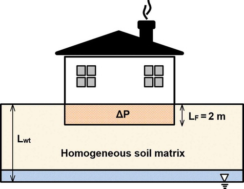
EPA’s version of J&E model (groundwater contamination advanced model, GW-ADV-Feb04.xls; EPA, 2004) was used to run simulations. This version of the J&E model is the most commonly used vapor intrusion model and has a theoretical framework similar to that of the model described by Johnson and Ettinger (1991); however, it is constrained in several ways to control user inputs, including embedded values for chemical and soil properties (EPA, 2004). A conceptual description of the modeled scenarios is schematically illustrated in Figure 1. As seen in this figure, the depth of basement (L_F) is considered 2 m. In order to simplify the simulation process, it is assumed that the subsurface consists of one homogenous soil type and the source is contaminated groundwater.

Figure 1. Conceptual description of modeled scenarios. Gray zone indicates capillary fringe. Moisture content and thickness of the capillary zone are predefined in the model (EPA, 2004).

Table 1 provides additional information on model parameters. The selection of which input parameters would be modeled as random variables (instead of fixed-value inputs) was determined based on several factors. The source chemical determines the air–water partitioning (Henry’s constant at reference temperature) and the pure phase diffusivity of the chemical in air and water. For recalcitrant VOCs, these values are fairly consistent and typically vary less than one order of magnitude. Therefore, these two parameters were fixed and were based on a common vapor intrusion chemical, tetrachloroethene (PCE) (EPA, 2004). The building footprint and building height are also considered as fixed inputs because these can be physically measured in the field and therefore are less uncertain, as compared to other input parameters. In addition, according to Hers et al. (2003), crack ratio (crack size and geometry) is important in diffusion-only cases, and for average vapor flow rate into a building () greater than around 1 L/min, it doesn’t play an important role in the attenuation factor. This means that crack parameters could be assumed as deterministic values except for fine-grained soil types with deep contamination sources. Therefore, the present work does not examine effect of uncertainty in the crack-to-building-area ratio on the variability in the attenuation factor.

Table 2 shows a list of equations and dependent parameters in J&E model. Detailed information on parameters definition can be found in the User’s Guide of the EPA version of the J&E model (EPA, 2004). The α, which is defined as the ratio of indoor air concentration to the source concentration, depends on several inputs. These inputs are also functions of individual parameters that have to be estimated or measured directly. In this research, five parameters were selected to enter the model as random variables. These parameters include system temperature (T_s), source depth (L_wt), moisture content (θ_w), soil building pressure differential (ΔP), and indoor air exchange rate (ER). It is worth noting that effect of temperature was only considered in the equation for the Henry’s law constant due to the J&E model configuration. The role of temperature in vapor intrusion processes may warrant additional investigation of a kind not possible using the J&E model.

Table 2. Summary of governing equations

Equation	Parameter
	ER
	Soil type
	Soil type
	Soil type
	Soil type
	System temperature

Input parameters definition

The uncertainty within the model output is strongly affected by availability and quality of data on input parameters. From a probabilistic point of view, the available information and uncertainty about a parameter can be reflected in its probability distribution. In cases where there are limited data about a parameter, expert judgment can be used to assign a proper distribution. For instance, uniform random variables can be used when there are estimates about minimum and maximum values but no specific information is available on probability distribution between the two bounds or normal random variables can be utilized to represent unbiased measurement errors, when there is more confidence on the values around the mean (Isukapalli and Georgopoulos, 2001). In this research, based on published information, and considering the positivity of the model parameters, truncated normal distributions are assigned to the five uncertain parameters under consideration. The probability density function for a truncated normal random variable with mean and standard deviation confined to the interval (a, b) is given by the following equation:

(20)

in which is the probability density function for standard normal distribution is the corresponding cumulative density function, and appropriate choices of (a, b) allow for modeling randomness with positive support. Table 3 provides the necessary information for the random variables used to model uncertainty in this study. Three different source depths (shallow 3 m, medium 8 m, and deep 30 m) and three soil types (clay loam, sandy loam, and sand) were considered in order to cover a comprehensive range of relevant vapor intrusion cases. The data on mean values and range of variation for three of parameters including moisture content, pressure differential and air exchange rate were adopted from data available in the User’s Guide for EPA’s version of the J&E model. The interval for moisture variation of sand was assumed to be larger than the given values in the User’s Guide (EPA, 2004) in order to impose a limit to minimum and maximum values to have a compatible range and standard deviation; however, the values were low enough not to skew the results. Due to the lack of reliable information on the variances, they were assumed to be 10% of the mean value. For the cases where there is no range information available, the ranges were chosen such that mean ± standard deviation lies well within the range.

Table 3. Input parameters for Monte Carlo simulation

Soil type	Input Parameter	Mean	Standard deviation	Min	Max
Clay loam	(ºC)	10	10% mean	7	13
	Lwt (m)	3, 8, 30	10% mean	87.5% mean	112.5% mean
	(%)	0.168	10% mean	0.079	0.26
	(g/cm-sec^2)	50	10% mean	0	200
	ER (1/hr)	0.25	10% mean	0.18	1.26
Sandy Loam	(ºC)	10	10% mean	7	13
	Lwt (m)	3, 8, 30	10% mean	87.5% mean	112.5% mean
	(%)	0.103	10% mean	0.039	0.17
	(g/cm-sec^2)	50	10% mean	0	200
	ER (1/hr)	0.25	10% mean	0.18	1.26
Sand	(ºC)	10	10% mean	7	13
	Lwt (m)	3, 8, 30	10% mean	87.5% mean	112.5% mean
	(%)	0.054	10% mean	0.04	0.068
	(g/cm-sec^2)	50	10% mean	0	200
	ER (1/hr)	0.25	10% mean	0.18	1.26

Notes: Mean, maximum, and minimum value for three parameters including moisture content, pressure differential, and air exchange rate were adopted from EPA (2004) User’s Guide for current version of J&E model. For the other two, reasonable values from the literature were assumed. For each input, the values for min, max, mean, and standard deviation were used to define the parameters of a truncated normal distribution.

As with any sensitivity analysis, the selection of specific ranges for input parameters influences the overall results. The authors selected values that are appropriate for the analysis and discussion provided herein. Future work could consider other ranges for input parameters to gain added insight about situations where extreme conditions may exist. For instance, the soil moisture content could be varied over a broader range to consider the effect of saturated lenses; however, these types of conditions are not the focus of the present work. In order to achieve predictions relevant to realistic situations encountered in the field, the temporal and spatial variability of input parameters could be taken into account; however, such analysis requires a more sophisticated analysis (e.g., via stochastic fields).

Results and Discussion

Propagation of uncertainties

, soil total effective diffusivity and effective permeability were considered as three outputs for uncertainty analysis. It is worth noting that soil total effective diffusivity for the entire domain is obtained by lumping the diffusivity of two phases (water and gas) and soil porosity for every single soil layer. K_v is defined as permeability of open soil pore spaces and therefore depends on soil moisture content. Monte Carlo simulations were performed to estimate the pdf of these parameters for all scenarios. Figure 2 depicts the pdf of values in logarithmic scale. It should be mentioned that using a log-scale x-axis alters the real distributions of data—the qualitative illustration of spread and variability of parameters in any log graph doesn’t necessarily reflect the spread and variability of real data—but is used so model outputs are more readily observed.

Figure 2. Probability density function of α for all modeled scenarios (CL = clay loam, SL = sandy loam, S = sand); 3, 8, and 30 m refer to the depth of contamination source, L_wt.

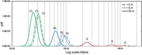
As expected, for all depths, clay loam and sand have the smallest and largest mean , respectively. It can be seen from Figure 2 that values for both clay loam and sandy loam do not show much variation for different depths (less than one-half log unit). In contrast, for sand the variability increases as source depth increases. Thus, it can be concluded that model output is more sensitive to source depth in coarse-grained soil types. Numerical values for variances also reveal that despite the fact that all input standard deviations are considered as 10% of mean value, variances of for all depths (3 m–30 m) are larger for sand than for clay loam and sandy loam. This is apparent in the data spread for each scenario.

Figures 3a and 3b show the pdfs for and values for all scenarios, respectively. depends on moisture content () as a random variable, but is a function of three random variables (see Table 1). This is apparent in the substantial difference in data variability between these two parameters (Figure 3a compared to Figure 3b).

Figure 3. Probability density function of (a) and (b) values for all modeled scenarios (CL = clay loam, SL = sandy loam, S = sand); 3, 8, and 30 m refer to the depth of contamination source, L_wt.

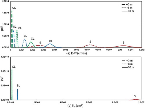
Figure 3a shows that for all soil types, mean increases as source depth increases and the relative increase in mean values for sand (3 m compared to 30 m depths) is approximately half an order of magnitude, as compared to mean values for sandy loam and clay loam, which increase more than one order of magnitude from a depth of 3 m to 30 m. The mean values for sand for 3 m, 8 m, and 30 m are 2.5E-3, 7.3E-3, and 1.03E-2 cm²/sec, respectively. The mean values for clay loam are 1.05E-4, 5.70E-4, and 1.9E-3, respectively, and are approximately a factor of 2 lower than the values for sandy loam. These data show that the mean values for sand are approximately an order of magnitude greater than clay loam (and sandy loam). Analysis of variances also shows that the variances of increase with increasing source depth. Variances of for sand are again larger than sandy loam (approximately 1E-7) and sandy loam variances (approximately 1E-8) are larger compared to clay loam (approximately 1E-9).

As seen in Figure 3b, the spread of data for is quite different than that for . The mean value doesn’t change with depth since is not a function of source depth. The mean values are as follows: for sand, 9.58E-8 cm²; for sandy loam, 5.34E-9 cm²; and for clay loam, 1.09E-9 cm². These data show that the mean value for sand is approximately two orders of magnitude greater than the value for clay loam and one order of magnitude greater than for sandy loam.

Model sensitivity—Sobol indices

To investigate sensitivity of the J&E vapor intrusion model output , Sobol indices for all five input parameters were calculated. Only first-order indices are presented. This is due to the important fact that considerable interaction between inputs was not detected using second-order and higher order indices (the sum of first order indices is approximately 1).

Figure 4a depicts the Sobol indices for all three source depths. The indices were calculated for each modeled scenario, each of which has a pdf defined by a soil type and a source depth (see Figures 2 and 3). The sensitivity index for air exchange rate is considerably greater than other indices in all scenarios, which indicates the importance of air exchange rates in the J&E model calculations. For example, the Sobol indices for air exchange rates across all three soil types are approximately 0.7, while the Sobol indices for T_s, L_wt, θ_w, and ΔP ranged from zero to 0.4. Clearly, accurate prediction of air exchange is important when using the J&E model to predict site conditions.

Figure 4. Sobol indices for (a) α as an output with five random inputs; (b) α as an output and , , and source depth (L_wt) as random inputs; (c) α as an output with three random inputs; temperature and air exchange rate are excluded. Note: CL = clay loam, SL = sandy loam, S = sand; 3, 8, and 30 m refer to the depth of contamination source, L_wt.

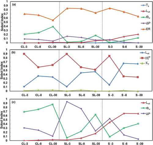
For clay loam (all source depths), air exchange rate and moisture content are important parameters and contribute most to the output variance. For sandy loam, the most influential parameters in shallow and medium depths are pressure differential and air exchange rate. Furthermore, moisture content becomes more important than pressure differential as depth increases. The indices for sand in shallow source depth show that after air exchange rate, the most important parameters affecting output variance are pressure differential and source depth, with nearly equal importance. As depth of contaminant source increases, the contribution of source depth in output variance becomes more noticeable for sand. The results support the conclusion that moisture content doesn’t play an important role in the variability of for coarse-grained soil types. Generally, as shown in Figure 4a, temperature does not have noticeable effect in output variance. As mentioned previously, the temperature term only appears in the Henry’s law constant equation in the J&E model and it therefore does not strongly affect the model output.

Total effective diffusivity versus effective permeability

To gain insight about importance of diffusivity and permeability estimation on the J&E model, input parameters were redefined, and three parameters including effective diffusivity, effective permeability, and source depth were considered in measuring the sensitivity of output. Sobol indices for these three parameters are illustrated in Figure 4b. For all scenarios, effective permeability index is considerably smaller than the diffusivity index. The parametric analysis by Johnson (2002, 2005) allowed manipulation of the three parameters (eqs 1–3) to evaluate the nature of the vapor intrusion transport process (advective vs. diffusive). The results shown in Figure 4b suggest that more attention should be paid to accurately estimating the total effective diffusivity of soil rather than permeability when evaluating vapor intrusion exposure risks using the J&E model. The importance of total effective diffusivity, as compared to source depth, is especially important for shallow soils (3 m). As the source depth increases to 8 m and 30 m, the model’s sensitivity to source depth increases. For sandy loam and clay loam, the model remains most sensitive to total effective diffusivity, but for sandy soils, the model is more sensitive to source depth for 8-m and 30-m scenarios, as compared to total effective diffusivity. Further, the total effective diffusivity of the soil matrix varies more greatly than permeability, irrespective of soil type and source depth. This finding is important in terms of applying the J&E model at hazardous waste sites and understanding the implications of grossly assumed input parameters.

It is noted that the uncertainty associated with the classification or evaluation of soil type/property may have a significant impact on the variability of model output. The intent of the research presented here, however, is not to assist a practitioner when using the EPA spreadsheets for a single site. Rather, the intent is to examine a wide range of vapor intrusion scenarios. The research findings are particularly useful for situations where soil types have a high level of uncertainty because the results are reported for a range of soil types, spanning from sand to clayey soils (see Figures 3 and 4).

Effect of source depth, moisture content, and pressure differential

As shown in Figure 4a, it is difficult to make a precise comparison between source depth, moisture content, and pressure differential because of the large effect of air exchange rate. Hence, a new set of simulations and sensitivity index calculations was performed with the aim of assessing the effect of source depth, moisture content, and pressure differential. The results are illustrated in Figure 4c and show that after air exchange rate, moisture content is the most important parameter for clay loam. Additionally, the Sobol index for moisture content increases as source depth increases, while pressure differential becomes less important. Sandy loam shows a different trend; in shallow and medium depth, model output has higher sensitivity to pressure differential, but surprisingly, in the deep case it switches to moisture content. It is apparent from Figure 4c that in sand and for shallow depth, pressure differential and source depth are of the same importance and model output becomes more sensitive to source depth as depth increases.

Summary

Through a systematic and scenario-based approach, this study provides important information about uncertainty in the J&E model output and its sensitivity to various inputs. Our uncertainty analysis suggests that the variability in the attenuation factor () was greatest for sand, followed by sandy loam and clay loam. This variation in values for specific depths differed less than one-half of an order of magnitude. However, across all soil types and all source depths, the model predicted attenuation factors that spread two orders of magnitude. For the sensitivity analysis, the robust variance decomposition technique used in this study was able to pinpoint the important factors affecting the J&E model predictions in a variety of settings, providing the vapor intrusion community with important information to consider when implementing the J&E model as part of hazardous waste site assessments. Importantly, and perhaps not surprisingly, our results identify high sensitivity to air exchange rate and call for more precise measurements of this quantity. Also, our results identify the role of total effective diffusivity in introducing uncertainty to J&E model output. In comparison to soil permeability, this parameter was shown to play a more important role for all soil types and source depths. Field measurements of total effective diffusivity are not commonly collected during vapor intrusion investigations; however, consideration of this parameter warrants additional attention and has been highlighted by others as important for vapor intrusion (Johnson, et al., 1998; Hers et al., 2009; Johnston and Gibson, 2011). Our results not only identify the range of variability to be expected depending on the scenario at hand, but also mark the important cases where special consideration should be given when estimating the input parameters to which the J&E model is most sensitive (i.e., ER, ).

Funding

The project described was supported by grants P42ES013660 (Brown University Superfund Research Program) and P42ES007380 (University of Kentucky Superfund Research Program) from the National Institute of Environmental Health Sciences.

Disclaimer

The content is solely the responsibility of the authors and does not necessarily represent the official views of the National Institute of Environmental Health Sciences or the National Institutes of Health.

Additional information

Funding

The project described was supported by grants P42ES013660 (Brown University Superfund Research Program) and P42ES007380 (University of Kentucky Superfund Research Program) from the National Institute of Environmental Health Sciences.

Notes on contributors

Ali Moradi

Ali Moradi received his MS in Civil & Environmental Engineering at the University of Massachusetts–Dartmouth under the co-advisement of Dr. Pennell and Dr. Tootkaboni. He is currently a doctoral student at the Colorado School of Mines.

Mazdak Tootkaboni

Mazdak Tootkaboni is an assistant professor in the Department of Civil & Environmental Engineering at the University of Massachusetts-Dartmouth.

Kelly G. Pennell

Kelly G. Pennell is an assistant professor in the Department of Civil Engineering at the University of Kentucky.

References

- Arwade, S.R., M. Moradi, and A. Louhghalam. 2010. Variance decomposition and global sensitivity for structural systems. Eng. Struct. 32(1): 1–10. doi:10.1016/j.engstruct.2009.08.011
- Colbert, K.L., and J.E. Palazzo. 2008. Vapor intrusion: Liability determination protects profits and minimize risk. Real Estate Finance 24:17–22.
- Dimov, I., and R. Georgieva. 2010. Monte Carlo algorithms for evaluating Sobol sensitivity indices. Math. Comput. Simulation 81:506–14. doi:10.1016/j.matcom.2009.09.005
- Eklund, B.M., and M.A. Simon. 2007. Concentration of tetrachloroethylene in indoor air at a former dry cleaner facility as a function of subsurface contamination: A case study. J. Air Waste Manage. Assoc. 57: 753–60. doi:10.3155/1047-3289.57.6.753
- Fishman, G.S. 1996. Monte Carlo: Concepts, algorithms, and applications. New York, NY: Springer Verlag.
- Hodgson, A., K. Garbesi, R. Sextro, and J.M. Daisey. 1992. Soil-gas contamination and entry of volatile organic compounds into a house near a landfill. J. Air Waste Manage. Assoc. 42(3): 277–83. doi:10.1080/10473289.1992.10466990
- Hers, I., R. Zapf-Gilje, L. Li, and J. Atwater. 2001. The use of indoor air measurements to evaluate intrusion of subsruface VOC vapos into buildings. J. Air Waste Manage. Assoc. 51(9): 1318–31. doi:10.1080/10473289.2001.10464356
- Hers, I., R. Zapf-Gilje, P.C. Johnson, and L. Li. 2003. Evaluation of the Johnson and Ettinger model for prediction of indoor air quality. Groundwater Monit. Remediation 23(2): 119–33. doi:10.1111/j.1745-6592.2003.tb00678.x
- Isukapalli, S.S., and P.G. Georgopoulos. 2001. Computational methods for sensitivity and uncertainty analysis for environmental and biological models. EPA/600/R-01-068. http://cfpub.epa.gov/si/si_public_record_report.cfm?dirEntryId=81032.
- Johnson, P.C. 2002. Identification of critical parameters for the Johnson and Ettinger (1991) vapor intrusion model. American Petroleum Institute, Technical Bulletin Number 17,38. http://www.api.org/environment-health-and-safety/clean-water/ground-water/vapor-intrusion/vi-publications/vapor-intrusion-model.
- Johnson, P.C. 2005. Identification of application-specific critical inputs for the 1991 Johnson and Ettinger vapor intrusion algorithm. Groundwater Monit. Remediation 25(1): 63–78. doi:10.1111/j.1745-6592.2005.0002.x
- Johnson, P.C., and R.A. Ettinger. 1991. Heuristic model for predicting the intrusion rate of contaminant vapors into buildings. Environ. Sci. Technol. 25:1445–52. doi:10.1021/es00020a013
- Johnson, P.C., C. Bruce, R.L. Johnson, and M.W. Kemblowski. 1998. In-situ measurement of effective vapor-phase porous media diffusion coefficients. Environ. Sci. Technol. 32: 3405–9. doi:10.1021/es980186q
- Johnston, J.E., and J. MacDonald Gibson. 2011.Probabilistic approach to estimating indoor air concentrations of chlorinated volatile organic compounds from contaminated groundwater: A case study in San Antonio, Texas. Environ. Sci. Technol. 45:1007–1013. doi:10.1021/es102099h
- Kroese, D.P., T. Taimre, and Z.I. Botev. 2011. Handbook of Monte Carlo methods. Hoboken, NJ: John Wiley & Sons.
- McAlary, T., and P.C. Johnson. 2009. Editorial: GWMR Focus issue on vapor intrusion. Ground Water Monit. Remediation 29(1): 40–41.
- National Research Council. 2005. Contaminants in the subsurface: Source zone assessment and remediation. Washington, DC: National Academies Press.
- Nazaroff, W.W. 1988. Predicting the rate of 222Rn entry from soil into basement of a dwelling due to pressure-driven air flow. Radiat. Protect. Dosim. 24:199–202.
- Pennell, K.G., O. Bozkurt, and E.M. Suuberg. 2009. Development and application of a three-dimensional finite element vapor intrusion model. J. Air Waste Manage. Assoc. 59: 447–60. doi:10.3155/1047-3289.59.4.447
- Picone, S., J. Valstar, P. van Gaans, T. Grotenhuis, and H. Rijnaarts. 2012. Sensitivity analysis on parameters and processes affecting vapor intrusion risk. Environ. Toxicol. Chem. 31(5): 1042–52. doi:10.1002/etc.1798
- Rubinstein, R.Y. 1981. Simulation and the Monte Carlo method. New York, NY: John Wiley & Sons.
- Saltelli, A. 2002. Making best use of model evaluations to compute sensitivity indices. Comput. Phys. Commun. 145(2): 280–97. doi:10.1016/S0010-4655(02)00280-1
- Schreüder, W.A. 2006. Uncertainty approach to the Johnson and Ettinger vapor intrusion model. Proceedings of the National Groundwater Association Ground Water and Environmental Law Conference, Chicago, IL, July.
- Sobol, I.M. 2001. Global sensitivity indices for nonlinear mathematical models and their Monte Carlo estimates. Math. Comput. Simulation. 55:271–80. doi:10.1016/S0378-4754(00)00270-6
- Tillman, F.D., and J.W. Weaver. 2006. Uncertainty from synergistic effects of multiple parameters in the Johnson and Ettinger (1991) vapor intrusion model. Atmos. Environ. 40: 4098–112. doi:10.1016/j.atmosenv.2006.03.011
- Tillman, F.D., and J.W. Weaver. 2007. Parameter sets for upper and lower bounds on soil-to-indoor-air contaminant attenuation predicted by the Johnson and Ettinger vapor intrusion model. Atmos. Environ. 41: 5797–806. doi:10.1016/j.atmosenv.2007.05.033
- U.S. Environmental Protection Agency. 2002. Draft guidance for evaluating the vapor intrusion to indoor air pathway from groundwater and soils. Washington, DC: U.S. PA.
- U.S. Environmental Protection Agency. 2004. User’s guide for evaluating subsurface vapor intrusion into buildings. Washington, DC:. EPA, Office of Emergency and Remedial Response. http://www.epa.gov/oswer/riskassessment/airmodel/pdf/2004_0222_3phase_users_guide.pdf (accessed August 2013).
- U.S. Environmental Protection Agency. 2012. EPA’s vapor intrusion database: Evaluation and characterization of attenuation factors for chlorinated volatile organic compounds and residential buildings (EPA 530-R-10-002). Washington, DC:. EPA, Office of Solid Waste and Emergency Response.
- Yu, S., A. Unger, and B. Parker. 2009. Simulating the fate and transport of TCE from groundwater to indoor air. J. Contam. Hydrol. 107:140–61. doi:10.1016/j.jconhyd.2009.04.009