Composition and sources of fine and coarse particles collected during 2002–2010 in Boston, MA

Abstract

Identifying the sources, composition, and temporal variability of fine (PM_2.5) and coarse (PM_2.5–10) particles is a crucial component in understanding particulate matter (PM) toxicity and establishing proper PM regulations. In this study, a Harvard Impactor was used to collect daily integrated fine and coarse particle samples every third day for 9 years at a single site in Boston, MA. In total, 1,960 filters were analyzed for elements, black carbon (BC), and total PM mass. Positive Matrix Factorization (PMF) was used to identify source types and quantify their contributions to ambient PM_2.5 and PM_2.5–10. BC and 17 elements were identified as the main constituents in our samples. Results showed that BC, S, and Pb were associated exclusively with the fine particle mode, while 84% of V and 79% of Ni were associated with this mode. Elements mostly found in the coarse mode, over 80%, included Ca, Mn (road dust), and Cl (sea salt). PMF identified six source types for PM_2.5 and three source types for PM_2.5–10. Source types for PM_2.5 included regional pollution, motor vehicles, sea salt, crustal/road dust, oil combustion, and wood burning. Regional pollution contributed the most, accounting for 48% of total PM_2.5 mass, followed by motor vehicles (21%) and wood burning (19%). Source types for PM_2.5–10 included crustal/road dust (62%), motor vehicles (22%), and sea salt (16%). A linear decrease in PM concentrations with time was observed for both fine (–5.2%/yr) and coarse (–3.6%/yr) particles. The fine-mode trend was mostly related to oil combustion and regional pollution contributions. Average PM_2.5 concentrations peaked in summer (10.4 µg/m³), while PM_2.5–10 concentrations were lower and demonstrated little seasonal variability. The findings of this study show that PM_2.5 is decreasing more sharply than PM_2.5–10 over time. This suggests the increasing importance of PM_2.5–10 and traffic-related sources for PM exposure and future policies.

Implications: Although many studies have examined fine and coarse particle composition and sources, few studies have used concurrent measurements of these two fractions. Our analysis suggests that fine and coarse particles exhibit distinct compositions and sources. With better knowledge of the compositional and source differences between these two PM fractions, better decisions can be made about PM regulations. Further, such information is valuable in enabling epidemiologists to understand the ensuing health implications of PM exposure.

Introduction

In numerous epidemiological studies, exposure to airborne particulate matter (PM) has been associated with increased mortality as well as several adverse respiratory, cardiovascular, and neurological conditions (Pope and Dockery, 2006; Roberts et al., 2013). In many such studies, exposure is usually characterized based on measured mass concentration of particles within specific size ranges. Typically, these include particles with an aerodynamic diameter of less than 10 µm (PM₁₀), less than 2.5 µm (PM_2.5), and between 2.5 and 10 µm (PM_2.5–10), also known as inhalable, fine, and coarse particles, respectively. Though valuable, this approach does not take into account the chemical compositions of particles and is therefore unlikely to tell the entire story as it relates to human health effects resulting from airborne particle exposure. Recent literature suggests that chemical components such as metals, elemental carbon, and organic carbon compounds, among others, may play an important role in particle toxicity (Fanning et al., 2009; Lippmann, 2010). Epidemiological studies have provided some evidence about the importance of this particle composition, as is the case in a new study showing an association between autism spectrum disorder and exposure to airborne metals and diesel particles (Roberts et al., 2013). Other studies have linked components such as sulfur, copper, nickel, zinc, organic carbon (OC), and black carbon (BC), either alone or in mixtures, to increased cardiovascular disease and mortality (Vedal et al., 2013; Flemming et al., 2013; Valdes et al., 2012; Lippmann & Chen, 2009). Clinical and toxicological studies have also shown associations between specific PM components and physiological outcomes (Araujo et al., 2010). To date, a consensus has not surfaced as to precisely which constituents elicit specific outcomes.

Due to its chemical and biological composition, residence time, and ability to penetrate deep into the lung, PM_2.5 has received deserved attention in the media as well as within the political and scientific arenas. This is reflected by the 2012 revision of the U.S. National Ambient Air Quality Standards (NAAQS) for PM, in which the primary annual PM_2.5 standard was lowered from 15.0 to 12.0 µg/m³. Also, clinical and toxicological studies have reported that coarse particles resulting from road dust (mixed debris from brake wear, tire wear, road abrasion, and biological and geological matter) can be as toxic as fine particles on a mass basis (Thorpe and Harrison, 2008; Flemming, 2012). As the role of particle composition in producing toxicity is uncovered, it is increasingly important to investigate the compositional differences between PM_2.5 and PM_2.5–10, as well as identifying their sources. This is of particular importance in urban settings, where traffic-related PM is higher and coarse particles are largely made up of resuspended road dust (Manoli et al., 2002).

Studies aimed at understanding the origin of ambient PM have been conducted in various cities around the world. In some studies, source apportionment was conducted without considering coarse particles (Kim et al., 2005; Gugamsetty et al., 2012), while in other studies, fine and coarse particles are not collected concurrently, or are not collected in areas that reflect large-scale urban air (Khodeir et al., 2012; Davy et al., 2012). When fine PM and coarse PM are measured concurrently, source apportionment studies are still often limited in terms of their sample size and study length (Gietl et al., 2009; Dordevic et al., 2012; Clements et al., 2014; Contini et al., 2014), analyzing fewer than 200 samples and spanning a few years or less. The objective of this study is to analyze nearly 2,000 daily integrated particle samples collected every third day for a 9-year period in order to investigate the composition of PM_2.5 and PM_2.5–10 at a single urban monitoring site (Boston, MA). Additionally, we aim to identify and quantify the source contributions of PM_2.5 and PM_2.5–10 as well as explore their temporal trends. With greater knowledge of the source and compositional differences between these two PM fractions, and with better insight as to the annual trends and seasonal variability of such concentrations, epidemiologists will be better equipped to understand the ensuing health implications of PM exposure. Finally, we evaluate the seasonal and temporal tends in the fine and coarse mode during the sampling period and investigate their relation to changes in sources contributions. This information is valuable in enabling better decision making concerning PM regulations.

Methods

Particle sampling and chemical analysis

Daily PM samples were collected during 2002–2010 at the Harvard supersite in Boston, MA, with the exception of a 6-month period from June 2009 to Janurary 2010 when monitoring equipment became unavailable. The Boston supersite is located atop the six-story Countway Library building of the Harvard Medical School, and sits within one block of a four-lane roadway as well as near two major highways, namely, Interstate 90 (I-90), which is approximately 1.5 km to the north, and Interstate 93 (I-93), which is approximately 3 km to the south.

In total, 980 PM_2.5 and 980 PM₁₀ daily integrated samples were collected concurrently every third day on 37-mm Teflon filters using Harvard Impactors (Marple, 1987). Filters, including blanks, were weighed on an electronic microbalance (MT-5 Mettler Toledo, Columbus, OH) prior to and after field measurements, after being equilibrated for a period of 48 hr in a particle-free room of controlled temperature (22 ± 5°C) and relative humidity (4 0 ±5%). To eliminate the effects of static charge, the filters were passed over alpha ray sources prior to each weighing. Following gravimetric analysis, Teflon filters were analyzed using x-ray fluorescence (XRF) spectroscopy (model Epsilon 5, PANalytical, The Netherlands) to determine the elemental composition of the PM (U.S. Environmental Protection Agency [EPA], 1999). In total, 48 elements were measured. The elements measured were those that are standard for XRF analysis due to their detectability using this measurement technique. Quality assurance/quality control of XRF analyses is available in Kang et al. (2014). Black carbon (BC) concentrations were measured using a single (λ = 880 nm) channel aethalometer (model AE-16, Magee Scientific, Berkeley, CA). For days when aethalometer data were not available we measured BC using a smokestain reflectometer (model M43D, Diffusion Systems Ltd., United Kingdom). PM_2.5 organic carbon (OC) measurements were collected from 2007 to 2010 using a semicontinuous carbon aerosol analyzer (model 3, Sunset Laboratory, Tigard, OR), which uses a carbon-impregnated parallel plate organic denuder designed to remove gaseous organic compounds upstream of the collection filter (Kang et al., 2010). The OC measurements consisted of 357 samples. Blank medians and limits of detection (LOD) for each component used in this work are available in the supplementary materials. All analyses were conducted at the Harvard School of Public Health.

Mass closure analysis and annual trends

To perform mass closure analyses, we converted the molar masses of each element into the molar masses of their common oxides, since they rarely exist as pure elements in the environment. The oxides we accounted for included Al₂O₃, SiO₂, K₂O, CaO, TiO₂, FeO, Fe₂O₃, and ZnO. The iron oxides FeO and Fe₂O₃ were considered to be present in roughly equal amounts (Taylor, 1964). Additionally, S was assumed to be (NH₄)₂SO₄ (ammonium sulfate) while Na and Cl were assumed to be bound as NaCl (sea salt). For PM_2.5, we also accounted for BC and OC mass. Since OC measurements were available for only 3 years, we used the OC/PM_2.5 mass fraction calculated during this time period to conduct mass closure for this species over the entire study duration. We also conducted mass closure when restricting all samples to the 3-year time period during which OC samples were collected; however there was little impact to our results. With the exception of OC in the case of PM_2.5, mass closure analyses only accounted for the species that were included in our PMF models.

Annual trends for coarse and fine particles were assessed by fitting a trend line to average annual coarse- and fine-mode PM concentrations. To assess relative percentage annual change in PM concentrations, annual PM averages were first natural log transformed and then regressed over time. The slope of this trend line represented the relative percent annual change. To estimate the impacts of individual sources to annual fine and coarse particle trends, we performed univariate regression analyses comparing these trends with and without the inclusion of the mass contributions of each source type separately, using two regression models shown by the following equations:

(1)

(2)

where log(PM_ij) is the natural logarithm of the mass concentration of particle size i, collected on sampling day j; β_tio is the time trend of PM_i concentrations before adjusting for the different source contributions; α_io is the intercept of the unadjusted model for size i; t is the time (in years) during which sample j was collected (e.g., t = 0 for year 2002, t = 1 for year 2003, etc.); α_ik is the intercept for the source contribution-adjusted model corresponding to particle size i and source k; β_tik is the time trend of PM_i concentrations after adjusting for the contribution of source k; f_ikj is the contribution of source k to the PM_i mass i on day j; and β_fik is the slope of f_ikj. In both models we controlled for month and weekday since concentrations depend on these two variables. Month_a and weekday_b are the month and weekday during which sample_j was collected. The time slope, β_tio, equals the relative percent change of either fine or coarse particle mass per year. β_tio is positive when concentrations are increasing and negative when concentrations are decreasing. Furthermore, β_tik equals the relative percent trend in either fine or coarse mass concentrations, should the contributions of source k remain constant. Therefore, the impact of source k on the PM_i mass concentration trend can be estimated using the following equation:

(3)

where ∆t_ik is the percent annual change in PM_i that is associated with the annual change in contributions of source k. If ∆t_ik is positive, then changes in contributions of source k resulted in an increase in PM_i mass concentrations. Negative values indicate that source k was responsible for a decrease. If ∆t_ik = 0, then source k had no effect.

Positive matrix factorization

To identify PM_2.5 and PM_2.5–10 sources and quantify their contributions, we used Positive Matrix Factorization (PMF) 3.0 software developed by the U.S. Environmental Protection Agency (Norris et al., 2008). PMF is a multivariate factor analysis tool that produces factor contributions and factor profiles based on inputted mass concentration files and estimated uncertainty files. In PMF, a speciated data set is interpreted as a data matrix X with dimensions j by l, where j and l represent the number of samples and chemical species measured, respectively. The model defines X_jl as follows (Gugamsetty et al., 2012):

(4)

where p is the number of factors, f is the species profile, g is the mass contribution, and e_jl is the error estimate for each sample. PMF enables for individual sample weighting that can account for missing or below-detection-limit data, which is common in environmental sampling (Song et al., 2001). This constitutes a major advantage of this model. Additionally, PMF output is constrained so as to allow no negative source contribution. The goal of PMF is to minimize the object function Q, which is defined as follows (EPA, 2008):

(5)

where x_jl denotes measured concentrations, u_jl denotes estimated uncertainty, n denotes the number of samples, m denotes the number of species, and p denotes the number of factors included in the model. PMF has been described in greater detail elsewhere (Paatero, 1997; Paatero and Tapper, 1994).

In our analysis, mass and elemental concentrations and their uncertainty values for PM_2.5 and PM₁₀ samples were obtained from our analytical environmental chemistry laboratory. PM_2.5–10 mass and elemental concentrations were estimated as the difference between their corresponding concentrations measured in PM₁₀ and PM_2.5 samples. Since PM_2.5–10 mass and elemental concentrations were not measured directly, uncertainties for PM_2.5–10 components were calculated by taking the square root of the sum of their corresponding squared PM₁₀ and PM_2.5 uncertainties. Elements with more than 50% of their concentration values below the limit of detection (LOD) were excluded from further analysis. Concentration values below the LOD were kept as is for elements that were further analyzed. Exceptions to this exclusion criterion were Cu and Ba, which we kept in our analysis because they are key tracer elements of vehicular wear debris (Lough et al., 2005; Garg et al., 2000; Hjortenkrans et al., 2007). For the remaining elements, negative concentration values were assumed to be zero, while zero uncertainty values were assumed to be 0.001 ng/m³ (the most conservative uncertainty based on XRF data that looked at multiple elements). Of 48 elements analyzed, 17 were included for further analysis while 31 elements were excluded.

Since aethalometer measurements for PM₁₀ BC were not available in this study, PM₁₀ BC was predicted. To this end, we investigated the relationship between a subset of our PM₁₀ and PM_2.5 BC samples, as measured by a reflectometer. This subset included 120 PM₁₀ and 120 PM_2.5 samples, and was analyzed in our environmental chemical laboratory. The mass relationship between PM₁₀ BC and PM_2.5 BC was slightly negative, suggesting that masking of dark BC particles by lighter particles had occurred. Masking may be more pronounced in PM₁₀ since it contains more light-reflective aerosols such as crustal minerals and salt particles. Given that a negative relationship with concurrently measured PM₁₀ and PM_2.5 BC is not possible, we assumed that BC instead accounted for a negligible mass fraction of coarse particles and therefore did not include PM_2.5–10 BC as a variable in our PMF analysis.

When running PMF, we distinguished between elements whose analysis was “bad” (signal-to-noise ratio < 0.2), “weak” (0.2 ≤ signal-to-noise ratio < 2), and “strong” (signal-to-noise ratio ≥ 2) (Paatero and Hopke, 2003). Species categorized as “bad” were eliminated from our analysis, while those considered “weak” were down-weighted by tripling their uncertainty values. “Strong” species were included in our analysis unchanged. Extreme concentrations that could be explained by episodic events such as firework celebrations were excluded from our analysis. Additional outliers were identified and excluded based on analysis of each species’ respective concentration time-series plot. Extreme values can be very influential since they may yield false factors/sources and/or distort source profiles.

PMF was run multiple times using four to eight factors for PM_2.5. For coarse particles, PMF was run using three to five factors, since fewer sources were expected for these particles. For a given model run, the converged solution with the lowest Q value in the robust mode was assessed in relation to its corresponding Q value in the nonrobust mode to ensure that remaining extreme values did not overly influence the model (Paatero, 2002). The PMF solutions chosen to represent PM_2.5 and coarse species were those deemed most physically reasonable and interpretable among all assessed solutions. Factors were then named according to the consideration of their abundance of key tracer elements, seasonal variability, and day-of-the-week contributions. Rotational ambiguity in solutions was explored using the FPEAK parameter ranging from –2 to 2, with the standard values of zero being the final choice. Goodness of fit for the PMF solutions was also examined by comparing predicted and measured concentration profiles for each species and their associated percent mean relative errors (MRE). MRE is equal to the absolute value of [(measured concentration – predicted concentration)/measured concentration]. This produces an easily interpretable error that is in the form of a fraction of measured values. The p values reported in this study were produced from a paired t-test when assessing weekday/weekend variability and from Scheffé’s method for multiple comparisons when assessing seasonal variability of PMF source contributions.

Results and Discussion

Contribution of coarse particles to total PM₁₀ mass and elemental concentrations

Figure 1 depicts the percent contribution of coarse particles to PM₁₀ mass and elemental concentrations. This enables us to identify to what extent PM₁₀ constituents are associated with the coarse versus fine particle mode. BC, S, and Pb were exclusively associated with PM_2.5 particles. Similarly, 84% of V and 79% of Ni were associated with fine particles. Between 50% and 75% of Al, K, Br, and Ba measured in PM₁₀ was contributed by the coarse mode. These elements are the major constituents of crustal and road dust. The elements that are mostly found in the coarse mode, over 75%, included the crustal and road dust elements Ca, Si, Ti, Fe, and Mn as well as Cl (sea salt). Hueglin et al., (2005) found similar results for coarse particles, except for K and Ti, which were reportedly mostly in the fine mode. In terms of total mass, the coarse mode accounted for about one-third (5.0 µg/m³) and the fine mode accounted for two-thirds (9.5 µg/m³) of PM₁₀ (14.5 µg/m³) mass.

Figure 1. Relative contributions of coarse and fine particles to total PM₁₀ mass.

Mass closure analysis

Figure 2 depicts mass closure results for coarse- and fine-mode particles. The elements selected for PMF analysis, together with OC and BC, accounted for 98% of total measured PM_2.5 mass. This percentage takes into account the elements Al, Si, K, Ca, Ti, Fe, and Zn in their common oxidized forms (labeled as metal oxides), as well as Na and Cl (labeled as sea salt). S as an oxidized sulfate was also considered (labeled as ammonium sulfate). The majority of fine-mode mass was made up of (NH₄)₂SO₄ and OC, accounting for 44 and 40% of total mass, respectively. BC, metal oxides, and sea salt accounted for 7, 5, and 2% of mass, respectively. While only 2% of mass was characterized as unknown, it is likely that our mass closure for (NH₄)₂SO₄ represents an overestimate of this fraction, as not all sulfate particles exist as ammonium sulfate, but also as Na₂SO₄. If we assume all (NH₄)₂SO₄ instead exists as Na₂SO₄, our unknown fraction increases to 14%. The unknown mass of PM_2.5 is likely made up of unmeasured ammonium nitrate particles, trace metals, organic compounds, and crystalline water that we did not consider in this work.

Figure 2. Mass closure results for (a) fine and (b) coarse particles.

For coarse particles, our study elements represented 41% of total coarse mass. As with the fine mode, the same elements were considered in their compound forms. Metal oxides and sea salt were both enriched in the coarse mode relative to the fine mode, accounting for 28% and 8% of total coarse mass, respectively. This was expected, as wind-blown soil, dust, and sea salt minerals tend to be larger particles. Other inorganics, which included Mn, Cu, Br, and Ba, accounted for 5% of total mass. As S was not present in the coarse mode, we expect that the remaining mass fraction of coarse particles can be explained by unaccounted for soil organics, nitrate compounds, trace elements, carbonates/bicarbonates, and biological aerosols. This is similar to other analyses, which have shown trace elements, nitrates, elemental carbon, and organic matter to account for 24–40%, and unknown constituents 31–50%, of coarse mass, respectively (Hueglin, 2005). As described earlier, particle masking may have also led to an under prediction of BC in the coarse mode. Therefore, BC may comprise some of our unknown mass fraction.

Source contributions of fine-mode particles

PMF analysis identified six factors for fine-mode particles. These included regional pollution, motor vehicles, sea salt, crustal/road dust, oil combustion, and wood burning. The concentrations and source characterizations of the PM_2.5 constituents are presented in Table 1. Regional pollution was the major source contributor to PM_2.5 mass, accounting for 48%. This source type was characterized using sulfur as a tracer, since the atmospheric conversion of sulfur dioxide to sulfate particles is sufficiently slow that sulfate is not generated locally, but usually over long-range transport (Wojcik and Chang, 1997; Kang et al., 2010; Seinfeld and Pandis, 2006). Our analysis also shows sodium to be associated with regional pollution. This is likely a result of chloride depletion chemistry taking place in the atmosphere during transport and on sampling filter surfaces (Zhao and Gao, 2008; McInnes et al., 2012; Lee et al., 2011). That is, as acid sulfate particles H₂SO₄ and NH₄HSO₄ are transported (or collected on the Teflon filters) they react with neighboring NaCl molecules to form Na₂SO₄ and HCl. Since HCl is a gas it reenters the air, leaving only Na₂SO₄ to be measured on the filter. Similar chloride depletion can occur through reactions involving nitrate and organic acids (Zhao and Gao, 2008; Kouyoumdjian et al., 2006). These phenomena, either alone or in combination, could be responsible for the association we observed between S and Na.

Table 1. Source contributions to fine particle mass and elemental concentrations (ng/m³) at Harvard Supersite

	Regional pollution	Motor vehicles	Sea salt	Crustal/road dust	Oil combustion	Wood burning	Estimated	Measured	%MRE
BC	105	350	1	3	81	43	583	658	12
Na	69	0	18	5	30	21	174	195	11
Al	9	7	0	29	1	1	47	47	1
Si	3	12	0	52	0	0	67	67	0
S	729	151	2	10	66	12	971	980	1
Cl	0	1	14	0	0	0	15	15	2
K	6	0	1	7	0	23	37	37	0
Ca	1	9	1	13	4	1	28	29	3
Ti	0	1	0	1	0	0	3	3	0
V	0	0	0	0	3	0	3	3	1
Fe	0	37	0	17	6	0	61	61	1
Ni	0	0	0	0	2	0	2	3	2
Cu	0	2	0	1	0	1	3	4	8
Zn	0	5	0	0	2	3	10	11	9
Pb	1	1	0	1	1	1	5	5	9
PM2.5	4,220	1,836	48	383	663	1,648	8,798	9,353	6

Regional pollution showed seasonal variability, ranging from 3.3 to 6.3 µg/m³. Summer showed the highest source contribution, with a difference in contribution that was statistically significant from all other seasonal contributions (p < 0.05). No other season had a significantly different contribution relative to other seasons. The summer peak of this source contribution was expected as atmospheric photochemical activity is at its peak during summer months, which translates to an increased conversion rate of emitted sulfur dioxide to sulfate particles. As expected, there was no difference in this source contribution between weekdays and weekends.

The motor vehicles factor was the second highest contributor to PM_2.5 mass, accounting for 21%. This source accounted for 60% of BC mass and was also characterized by the elements Zn, Fe, Ti, and Cu. Seasonal variability was observed, ranging from 1.5 to 2.2 µg/m³. The highest source contribution was for fall season, followed by spring and then winter. Fall and summer were significantly different from spring, and fall was also significantly different from winter (p < 0.05). Wind speed, boundary height, and precipitation partially accounted for these differences. Motor vehicles contributed more during weekdays than weekends (p < 0.0001) because vehicle emissions increase with weekday commuter traffic.

The source contribution of wood burning followed that of motor vehicles, accounting for 19% of PM_2.5 mass. This factor was characterized using K as a tracer, as this element is emitted during the combustion of wood and other forms of biomass (Fine et al., 2001; Khalil and Rasmussen, 2003). Wood burning is sometimes associated with quantities of Cl as well. That there is no Cl associated with this source type in our analysis may be due to the close proximity of the Atlantic Ocean, which serves as a much more dominant source of Cl. Alternatively, it could be due to chloride depletion chemistry, suggesting that wood-burning sources could be originating from further away. The source contribution ranged from 1.4 to 2.4 µg/m³, showing a statistically significant increase in contribution during winter relative to all other seasons (p < 0.05). This increase is likely a result of greater firewood use for residential heating during the cold season. A statistically significant increase in wood burning source type was also observed during weekends relative to weekdays (p < 0.001). As residential heating is an at-home activity, this increase is likely a reflection of the increase in hours spent at home during weekends, in addition to outdoor activities such as barbeques.

The oil combustion factor represented 8% of PM_2.5 mass and was characterized by its large contribution to oil tracer elements Ni and V. Oil combustion varied by season and ranged from 0.5 to 0.9 µg/m³, with a significantly higher contribution during winter months compared to all other seasons (p < 0.05). Sources of oil combustion include oil-fired power plants, ships, and ferries, as well as homes and commercial buildings (for heating). The higher contribution of oil combustion during winter is likely due to wintertime heating of homes and buildings that burn oil, as opposed to natural gas or biomass, for fuel (Spengler, 1983). This is expected, as a large proportion of Massachusetts residents (31%) tend to use oil for space heating (Energy Information Administration [EIA], 2014). This factor showed no significant difference in contribution when comparing weekdays and weekends, even when looking only within winter months.

Crustal/road dust factor accounted for 4% of PM_2.5 mass and was mostly associated with Al, Si, Ca, and Ti. Often, Zn and Fe are more heavily associated with road dust, suggesting that this source type may be a mixture of crustal matter and road dust. The contribution of this source type varied by season and ranged from 0.3 in fall to 0.5 µg/m³ in spring. Both spring and summer showed statistically high crustal/road dust contributions (p < 0.05). The higher source contribution during spring can be explained by differences in seasonal wind speed. Mean wind speed was highest during the spring (5.3 m/sec), with significant differences (p < 0.05) compared to fall (4.7 m/sec) and summer (4.3 m/sec). However, wind speed cannot explain the high source contribution during the summer as this season had the lowest mean wind speed. A likely factor influencing summertime contribution is temperature. During summer months, elevated temperatures lead to soil dryness, which contributes to particle resuspension. This factor also demonstrated a statistically significant increase in contribution during weekdays relative to weekends (p < 0.001). This increase is likely due to an increase in particle resuspension from higher roadway traffic by commuters during the work week.

The sea salt factor contributed the least, accounting for less than 1% of total PM_2.5 mass. As sea salt is composed mainly of Na and Cl, these elements are used as tracers of this source. However, in our analysis, sea salt was characterized mostly by the presence of Cl, as Na was better associated with regional sulfur as described earlier. Sea salt contribution ranged from zero to 0.1 µg/m³. While the highest contributions occurred during fall and spring, followed by winter, these differences were mostly not significant. Except for the fall season, the sea salt contribution was higher during seasons of higher mean wind speed. Elevated salt contributions during winter and spring may also be due to the use of sea salt as a deicing agent along roadways and sidewalks. There was no significant difference in sea salt contribution between weekdays and weekends, as expected.

Source contributions of coarse-mode particles

PMF analysis identified three factors for coarse-mode particles. These included crustal/road dust, motor vehicles, and sea salt. The concentrations and source characterizations of PM_2.5–10 constituents are presented in Table 2. Crustal/road dust was by far the major contributor to coarse particle mass, accounting for 62%, and was characterized by Al, Si, K, Fe, Ba, Zn, Mn, and Ti. While K in the fine mode is mostly associated with wood burning, in the coarse fraction it is related to road dust and soil. Though Fe is a major crustal element, the Fe/Si ratio of this source type was considerably higher than that of earth’s crust, suggesting a mixture of both soil and road dust (Taylor, 1964). The enrichment of Fe in road dust is related to traffic, since this element is typically present in brake-wear dust (Thorpe and Harrison, 2008; Pant and Harrison, 2013). The source contribution of this factor showed seasonal variability, ranging from 2.3 to 3.4 µg/m³. Spring and summer had significantly high crustal/road dust contributions relative to fall and winter months (p < 0.05). As with fine particles, the reason is likely due to high wind in the spring and elevated temperatures during summer. Also, partially thawed snow and wet road surfaces during winter months may reduce particle resuspension. This factor demonstrated a significant increase in contribution during weekdays relative to weekends (p < 0.0001). Similar to PM₂₅, this can be explained by an increase in resuspended particles from increased roadway traffic during the work week.

Table 2. Source contributions to coarse particle mass and elemental concentrations (ng/m³) at Harvard Supersite

	Crustal/road dust	Motor vehicles	Sea salt	Estimated	Measured	%MRE
Na	21	17	99	137	155	12
Al	98	14	5	117	115	2
Si	235	40	0	275	273	1
Cl	3	9	245	258	263	2
K	38	8	5	51	52	1
Ca	24	101	0	125	125	0
Ti	9	3	0	12	12	0
Mn	2	1	0	4	4	12
Fe	143	56	4	203	211	4
Cu	2	2	0	3	3	6
Zn	2	2	0	4	5	10
Br	1	1	0	2	3	21
Ba	11	9	1	21	27	21
PM2.5–10	2,782	981	732	4,495	5,049	11

The motor vehicles factor contribution was much less than that of crustal/road dust, accounting for 22% of total coarse mass. This factor was characterized by the elements Cu, Ca, and Br, which are associated with gasoline and oil combustion as well as tire and brake wear (Lough et al., 2005; Garg et al., 2000; Hjortenkrans et al., 2007). In the context of vehicle emissions, Ca is related to combustion of motor oil additives and lubricant oil, although its presence could also suggest some overlap with the crustal/road dust factor (Lough et al., 2005; Garg et al., 2000; Cadle et al., 1997). Counter to PM_2.5, the motor vehicles source showed no seasonal variability for coarse particles, remaining at 0.7 µg/m³ across all seasons. However, the contribution was significantly higher during weekdays than weekends (p < 0.001), again reflecting decreased vehicle traffic during weekends.

In contrast to our PM_2.5 analysis, sea salt contributed substantially to coarse particle mass, accounting for 16% of total mass. This is expected since sea salt particles primarily exist in the coarse mode (Harrison, 1983; Herner, 2006). Sea salt contribution varied by season (p < 0.0001) and ranged from 0.4 to 1.5 µg/m³. The greatest contribution occurred during winter months, which was significantly different relative to all other seasons (p < 0.05). Summer also showed a significantly lower contribution compared to fall (p < 0.05). This could be due to higher wind speeds during other months (summer had the lowest average wind speed), leading to greater ocean turbulence and the increased aerosolization of salt particles (Contini et al., 2010). Additionally, the increased contribution during winter could be due to the wintertime application of sea salt as a deicing agent to roadways and sidewalks. As expected, there was no significant difference in source contribution between weekdays and weekends.

Annual and seasonal PM

Annual averages of coarse- and fine-mode particles as well as source contributions to annual trends were assessed using eqs 1–3. Depictions of annual average trends for both particle size fractions are presented in Figure 3. A significant linear decrease in PM concentrations with time was observed for both coarse (p < 0.0001) and fine (p < 0.0001) particles, though the decrease was more pronounced for fine particles. Average annual PM_2.5 concentrations were highest (11.1 µg/m³) in 2002 and lowest (7.2 µg/m³) in 2010, showing an annual average decrease of 5.2% per year over our study period. This was mostly due to decreases in oil combustion and regional pollution source types, which accounted for a decrease equal to 59 and 47% of the annual decrease, respectively. The decrease in oil combustion sources could be reflecting the replacement of oil with natural gas for domestic heating. The motor vehicle source accounted for 30% of the annual decrease, while crustal/road dust contributed to only a 4% decrease. Wood burning contributed positively, with an annual increase of 14%. That is, the contribution of this source increased over our study period, counteracting the decreases seen across other sources. Sea salt did not affect the annual trend. After controlling for our various source types, a 26% increase in annual PM concentrations is unexplained. This could be due to PM constituents not included in our PMF analysis, such as bioaerosols and ammonium nitrate, as well as uncertainties in our PMF model estimates.

Figure 3. Annual average concentrations and standard deviations of (a) fine and (b) coarse particles.

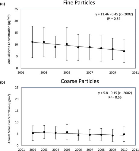
Average annual PM_2.5–10 concentrations were at a maximum (5.8 µg/m³) in 2003 and a minimum (4.3 µg/m³) in 2009. The average annual decrease for this mode was 3.6% per year. The factor that contributed most to this trend was crustal/road dust, accounting for 17% of the annual decrease, while sea salt and motor vehicles contributed negligibly to the trend. This left 83% of the annual decrease unexplained by our source types. This is not surprising, given our mass closure and PMF analyses, which showed a high fraction of unexplained mass and higher %MRE values for coarse particles, respectively.

In general, the temporal trends observed in this study can be explained by a number of factors, such as the replacement of oil with natural gas for wintertime heating and the replacement of old with new vehicles in the city. Regarding traffic emissions, for example, in recent years the Massachusetts Bay Public Transportation system replaced many old buses with a new fleet. Just this year, Harvard University also replaced its entire M2 bus fleet with new automobiles. Additionally, many taxi companies in Boston are now using hybrid vehicles, which produce fewer tailpipe emissions. With regard to long-range transport, increased compliance with acid rain regulations has reduced sulfur emissions over time. The extent to which the source contribution trends in this study are generalizable to other locations depends on the specific source and size fraction of interest. Fine particles, particularly those originating from long-range sources, are more likely to reflect concentrations observed elsewhere in the Northeast. Coarse particles concentrations, by contrast, are known to be more geographically heterogeneous, given their rapid settling velocity, and are therefore difficult to extrapolate to other locations (EPA, 2009).

For seasonal trends (Figure 4), the fine mode demonstrated variability while the coarse mode did not. Average fine particle concentrations were highest during summer (11.7 µg/m³), followed by winter (9.6 µg/m³). During summer, there was a statistically significant difference in concentrations relative to all other seasons, while wintertime concentrations were significantly different only when compared to spring (p < 0.05). Spring and fall had average concentrations of 8.0 and 8.2 µg/m³, respectively. This is consistent with our PMF results and is likely due to the increased atmospheric photochemistry that occurs during summer. Elevated wintertime levels are likely due to increased oil combustion and wood burning for heating. While coarse particle concentrations were highest in spring (5.2 µg/m³) and lowest in winter (4.7 µg/m³), seasonal differences for this size fraction were not significant. The slightly elevated concentration observed during spring may nonetheless be attributable to the increased resuspension of particles by wind, as this season corresponded to the highest average wind speed.

Figure 4. Seasonal average concentrations of (a) fine and (b) coarse particles.

Conclusion

The chemical compositions and sources of ambient fine- and coarse-mode particles were studied in Boston over a 9-year period. The primary strengths of this study are the simultaneous collection of fine and coarse particles and the extended period over which samples were collected. Our results suggest that coarse and fine particles have very different elemental compositions, reflecting their different sources and mechanisms of formation, as well as different annual trends and seasonal variation.

Fine particles were associated mostly with regional pollution and accounted for two-thirds of PM₁₀ mass, while coarse particles accounted for one-third of PM₁₀ mass and consisted mostly of crustal/road dust elements. The coarse-mode contribution to PM₁₀ reported in our study is similar to that reported in many urban environments (Marloes et al., 2012; Querol et al., 2004). Particularly noteworthy was the exclusive association between the combustion products S and BC in the fine particle mode. Pb was also associated exclusively with the fine mode, while V and Ni were highly associated with this mode. These findings are similar to those of Hueglin et al. (2005), who reported more than 80% of both Pb and sulfate, and more than 60% of V and N, to be present in the fine mode in the near-city environment. The elements that were mostly found in the coarse mode included the crustal and road dust elements Ca, Si, Ti, Fe, and Mn, as well as Cl (sea salt), similar to that reported by Hueglin et al. (2005). The assessment of coarse particle composition and concentration on a location-by-location basis is important in understanding the potential health implications to a given population, since coarse particles often originate from local sources and are known to be geographically heterogeneous, in contrast to fine particles, which are more homogeneously dispersed over space (EPA, 2009).

For mass closure, the species we analyzed accounted for 98% of total PM_2.5 mass and 41% of total PM_2.5–10 mass. The majority of fine-mode mass was made up of OC and sulfate. For the coarse mode, particles were more enriched with metal oxides and sea salt as compared to the fine mode, accounting for 28 and 8% of total coarse mass, respectively. This was expected, as wind-blown soil, dust, and sea salt minerals tend to be larger particles. That coarse particles are enriched with metals has implications for coarse PM toxicity, as such metals have been implicated as key components responsible for the health effects associated with PM (Flemming et al., 2013; EPA, 2009).

An annual decrease in PM concentrations was observed for both coarse and fine particles, though the decrease was more pronounced for fine particles. That PM_2.5 is decreasing more sharply over time than PM_2.5–10 suggests that PM_2.5–10 and traffic-related sources will be of increasing importance to PM exposure and environmental policies as we move into the future. The annual decline for PM_2.5 was mostly due to decreases in regional pollution and oil combustion source types. This decline in major source contributions of PM_2.5 appears to reflect the success of environmental acid rain policies to curb sulfur emissions, as well as a gradual shift toward cleaner sources of fuel, such as natural gas, as the energy market changes. For PM_2.5–10, crustal/road dust contributed most to the annual decline. Fine-mode particles demonstrated seasonal variability, with the highest average concentrations occurring during summer and winter months. By contrast, coarse-mode particles did not exhibit seasonal variability.

PMF analysis identified six source types for PM_2.5 and three source types for coarse particles. Fine particle concentrations were predicted well by our factor analysis, as demonstrated by their low MREs. Regional pollution contributed the most to PM_2.5 concentrations, accounting for 48% by mass, followed by motor vehicles (21%), wood burning (19%), oil combustion (8%), crustal/road dust (4%), and sea salt (<1%). These results are similar to those reported elsewhere in the United States (Lee et al., 2011; Kim et al., 2004; Kim et al., 2005). Regional pollution accounting for nearly half of fine particle mass lends merit to ongoing efforts to curb sulfur emissions, such as the U.S. Department of Energy’s action in 2011 to convert the Northeast Home Heating Oil Reserve to ultra-low-sulfur diesel (ULSD), as well as the decisions by several northeastern states to begin requiring ULSD for heating (EIA, 2014). Overwhelmingly the greatest contributor to coarse mass was crustal/road dust (62%), followed by sea salt (16%) and motor vehicles (22%). These finding are similar to other studies that have found road dust and sea salt to contribute substantially to coarse-mode particles (Harrison, 1983; Herner, 2006).

Funding

This work was supported by the EPA Center for Particle Health Effects at the Harvard School of Public Health (grant RD-83479801-2), a National Institute of Environmental Health Sciences (NIEHS) Program grant (P30-ES000002), and an Ambient Particles and Cardiac Vulnerability in Humans grant (P01-ES009825). However, any opinions, findings, conclusions, or recommendations expressed herein are those of the authors and do not necessarily reflect the views of the supporters. Further, our supporters do not endorse the purchase of any commercial products or services mentioned in this publication.

Supplemental Materials

Supplemental materials for this article can be accessed at http://dx.doi.org/10.1080/10962247.2014.982307.

Additional information

Funding

This work was supported by the EPA Center for Particle Health Effects at the Harvard School of Public Health (grant RD-83479801-2), a National Institute of Environmental Health Sciences (NIEHS) Program grant (P30-ES000002), and an Ambient Particles and Cardiac Vulnerability in Humans grant (P01-ES009825). However, any opinions, findings, conclusions, or recommendations expressed herein are those of the authors and do not necessarily reflect the views of the supporters. Further, our supporters do not endorse the purchase of any commercial products or services mentioned in this publication.

Notes on contributors

Shahir Masri

Shahir Masri is a doctoral student, Choong-Min Kang is a research associate, and Petros Koutrakis is a professor in the Department of Environmental Health, Harvard School of Public Health, Boston, MA.

References

- Araujo, J.A. 2010. Particulate air pollution, systemic oxidative stress, inflammation, and atherosclerosis. Air Qual. Atmos. Health. 4:79–93. doi:10.1007/s11869-010-0101-8
- Cadle, S H., P.A. Mulawa, J. Ball, C. Donase, A. Weibel, J.C. Sagebiel, K.T. Knapp, and R. Snow. 1997. Particulate emission rates from in-use high-emitting vehicles recruited in Orange County, California. Environ. Sci. Tech. 31: 3405–12. doi:10.1021/es9700257
- Cassee, F.R., M.E. Heroux, M.E. Gerlofs-Nijland, and F.J. Kelly. 2013. Particulate matter beyond mass: recent health evidence on the role of fractions, chemical constituents and sources of emission. Inhal. Toxicol. 25: 802–12. doi:10.3109/08958378.2013.850127
- Clements, N., J. Eav, M. Xie, M.P. Hannigan, S.L. Miller, W. Navidi, J.L. Peel, J.J. Schauer, M.M. Shafer, and J.B. Milford. 2014. Concentrations and source insights for trace elements in fine and coarse particulate matter. Atmos. Environ. 89:373–81. doi:10.1016/j.atmosenv.2014.01.011
- Contini, D., D. Cesari, A. Genga, M. Siciliano, P. Ielpo, MR. Guascito, and M. Conte. 2014. Source apportionment of size-segregated atmospheric particles based on the major water-soluble components in Lecce (Italy). Sci. Tot. Environ. 472: 248–61. doi:10.1016/j.scitotenv.2013.10.127
- Contini, D., A. Genga, D. Cesari, M. Siciliano, A. Donateo, M.C. Bove, and M.R. Guascito. 2010. Characterisation and source apportionment of PM10 in an urban background site in Lecce. Atmos. Res. 95:40–54. doi:10.1016/j.atmosres.2009.07.010
- Davy, P.K., T. Ancelet, W.J. Trompetter, A. Markwitz, and D.C. Weatherburn. 2012. Composition and source contributions of air particulate matter pollution in a New Zealand suburban town. Atmos. Pollut. Res. 3:143–47. doi:10.5094/APR.2012.014
- Dordevic, D., A. Mihajlidi-Zelic, D. Relic, Lj. Ignjatovic, J. Huremovic, and A.M. Stortini. 2012. Size-segregated mass concentration and water soluble inorganic ions in an urban aerosol of the Central Balkans (Belgrade). Atmos. Environ. 46: 309–17. doi:10.1016/j.atmosenv.2011.09.057
- Energy Information Administration. 2014. Massachusetts state profile and energy estimates. http://www.eia.gov/state/?sid=MA 2014 (accessed September 26, 2014).
- Fanning, E.W., J.R. Froines, M.J. Utell, M. Lippmann, G. Oberdorster, M. Frampton, J. Godleski, and T.V. Larson. 2009. Particulate matter (PM) centers (1999–2005) and the role of interdisciplinary center-based research. Environ. Health Perspect. 117:167–74. doi:10.1289/ehp.11543
- Fine, P.M., G.R. Cass, and B.R.T. Simoneit. 2001. Chemical characteristics of fine particle emissions from the fireplace combustion of woods grown in the southern United States. Environ. Sci. Tech. 36: 1442–51. doi:10.1021/es001466k
- Flemming, C.R., M. Heroux, M.E. Gerlofs-Nijland, and F.J. Kelly. 2013. Particulate matter beyond mass: Recent health evidence on the role of fractions, chemical constituents and sources of emission. Inhal. Toxicol. 25:802–12. doi:10.3109/08958378.2013.850127
- Garg, B., S.H. Cadle, P.A. Mulawa, P.J. Groblicki, C. Laroo, and G.A. Parr. 2000. Brake wear particulate matter emissions. Environ. Sci. Technol. 34:4463–69. doi:10.1021/es001108h
- Gietl, J.K., and O. Klemm. 2009. Source identification of size-segregated aerosol in Munster, Germany, by factor analysis. Aerosol Sci. Technol. 43: 828–37. doi:10.1080/02786820902953923
- Gugamsetty, B., H. Wei, C.N Liu, A. Awasthi, S.C. Hsu, C.J. Tsai, G.D. Roam, Y.C. Wu, and C.F. Chen. 2012. Source characterization and apportionment of PM10, PM2.5 and PM0.1 by using Positive Matrix Factorization. Aerosol Air Qual. Research. 12: 476–91. doi:10.4209/aaqr.2012.04.0084
- Harrison, R.M., and C.A. Pio. 1983. Size-differentiated composition of inorganic atmospheric aerosols of both marine and polluted continental origin. Atmos. Environ. 17:1733–38. doi:10.1016/0004-6981(83)90180-4
- Herner, J.D, Q. Ying, J. Aw, O. Gao, and D.P.Y. Chang. 2006. Dominant mechanisms that shape the airborne particle size and composition distribution in Central California. Aerosol Sci. Technol. 40:827–44. doi:10.1080/02786820600728668
- Hjortenkrans, D.S.T., B.G. Bergback, and A.V. Haggerud. 2007. Metal emissions from brake linings and tires: Care studies of Stockholm, Sweden 1995/1998 and 2005. Environ. Sci. Technol. 41:5224–30. doi:10.1021/es070198o
- Hueglin, C., R. Gehrig, U. Baltensperger, M. Gysel, C. Monn, and H. Vonmont. 2004. Chemical characterization of PM2.5, PM10 and coarse particles at urban, near-city, and rural sites in Switzerland. Atmos. Environ. 39:637–51. doi:10.1016/j.atmosenv.2004.10.027
- Kang, C.M., P. Koutrakis, and H.H. Suh. 2010. Hourly measurements of fine particulate sulfate and carbon aerosols at the Harvard–U.S. Environmental Protection Agency supersite in Boston. J. Air Waste Manage. Assoc. 60:1327–34. doi:10.3155/1047-3289.60.11.1327
- Kang, C.M., S. Achilleos, J. Lawrence, J.M. Wolfson, P. Koutrakis. 2014. Interlab comparison of elemental analysis for low ambient urban PM2.5 levels. Environ. Sci. Technol. 48:12150–6. doi:10.1021/es502989j
- Khalil, M.A.K., and R.A. Rasmussen. 2003. Tracers of wood smoke. Atmos. Environ. 37:1211–22. doi:10.1016/S1352-2310(02)01014-2
- Khodeir, M., M. Shamy, M. Alghamdi, M. Zhong, H. Sun, M. Costa, L.C. Chen, and P. Maciejczyk. 2012. Source apportionment and elemental composition of PM25 and PM10 in Jeddah City, Saudia Arabia. Atmos. Poll. Research. 3:221–40. doi:10.5094/APR.2012.037
- Kim, E., and P.K. Hope. 2004. Improving source identification of fine particles in a rural northeastern U.S. area utilizing temperature-resolved carbon fractions. J. Geophys. Res. 109:1984–2012. doi:10.1029/2003JD004199
- Kim, E., P.K. Hope, D.M. Kenski, and M. Koerber. 2005. Sources of fine particles in a rural Midwestern U.S. area. Environ. Sci. Technol. 39: 4953–60. doi:10.1021/es0490774
- Kouyoumdjian, H., and N.A. Saliba. 2006. Mass concentration and ion composition of coarse and fine particles in an urban area in Beirut: Effect of calcium carbonate on the absorption of nitric and sulfuric acids and the depletion of chloride. Atmos. Chem. and Phys. 6:1865–77. doi:10.5194/acp-6-1865-2006
- Lee, H.J., J.F. Gent, B.P. Leaderer, and P. Koutrakis. 2011. Spatial and temporal variability of fine particle composition and source types in five cities of Connecticut and Massachusetts. Sci. Total Environ. 409:2133–2142. doi:10.1016/j.scitotenv.2011.02.025
- Li, W.J., Z.B. Shi, C. Yan, L.X. Yang, C. Dong, and W.X. Wang. 2013. Individual metal-bearing particles in a regional haze caused by firecracker and firework emissions. Sci. Total Environ. 443:464–69. doi:10.1016/j.scitotenv.2012.10.109
- Lippmann M., and L.C. Chen. 2009. Health effects of concentrated ambient air particulate matter (CAPs) and its components. Crit. Rev. Toxicol. 39: 865–913. doi:10.3109/10408440903300080
- Lippmann, M. 2010. Targeting the components most responsible for airborne particulate matter health risks. J. Expos. Sci. Environ. Epidemiol. 20: 117–18. doi:10.1038/jes.2010.1
- Lough, G.C., J.J. Schauer, J.-S. Park, M.M. Shafer, J.T. Deminter, and J.P. Weinstein. 2005. Emissions of metals associated with motor vehicle roadways. Environ. Sci. Technol. 39:826–36. doi:10.1021/es048715f
- Manoli, E., D. Voutsa, and C. Samara. 2002. Chemical characterization and source identification/apportionment of fine and coarse air particles in Thessaloniki, Greece. Atmos. Environ. 36:949–61. doi:10.1016/S1352-2310(01)00486-1
- Marloes, E., M.Y. Tsai, C. Ampe, B. Anwander, R. Beelen, T. Bellander, G. Cesaroni, M. Cirach, J. Cyrys, K. de Hoogh, A. de Nazelle, et al. 2012. Spatial variation of PM2.5, PM10, PM2.5 absorbance and PMcoarse concentrations between and within 20 European study areas and the relationship with NO2—Results of the ESCAPE project. Atmos. Environ. 63:303–17. doi:10.1016/j.atmosenv.2012.08.038
- Marple, V., K. Rubow, W. Turner, and J. Spengler. 1987. Low flow rate sharp cut impactors for indoor air sampling: Design and calibration. J. Air Pollut. Control Assoc. 37:1303–7. doi:10.1080/08940630.1987.10466325
- McInnes, L.M., D.S. Covert, P.K. Quinn, and M.S. Germani. 2012. Measurements of chloride depletion and sulfur enrichment in individual sea-salt particles collected from the remote marine boundary layer. J. Geophys. Research. 99:8257–68. doi:10.1029/93JD03453
- Norris, G., R. Vedantham, K. Wade, S. Brown, J. Prouty, and C. Foley. 2008. EPA Positive Matrix Factorization (PMF) 3.0: Fundamentals & User Guide. U.S. Environmental Protection Agency. http://lasher.ouhsc.edu/oeh5743%5Cpmf.pdf (accessed November 4, 2014).
- Paatero, P. 1997. Least squares formulation of robust non-negative factor analysis. Chemometrics Intelligent Lab. Syst. 37:23–35. doi:10.1016/S0169-7439(96)00044-5
- Paatero, P., P.K. Hopke, X.H. Song, and Z. Ramadan. 2002. Understanding and controlling rotations in factor analytic models. Chemom. Intell. Lab. Syst. 60:253–64. doi:10.1016/S0169-7439(01)00200-3
- Paatero, P., and U. Tapper. 1994. Positive matrix factorization: A non-negative factor model with optimal utilization of error estimates of data values. Environmetrics. 5:111–26. doi:10.1002/env.3170050203
- Paatero, P., and P. K. Hopke. 2003. Discarding or downweighting high-noise variables in factor analytic models. Anal. Chim. Acta. 490:277–89. doi:10.1016/S0003-2670(02)01643-4
- Pant, P., and R.M. Harrison. 2013. Estimation of the contribution of road traffic emissions to particulate matter concentrations from field measurements: A review. Atmos. Environ. 77:78–97. doi:10.1016/j.atmosenv.2013.04.028
- Pope, C.A., and D.W. Dockery. 2006. Health effects of fine particulate air pollution: Lines that connect. J. Air Waste Manage. Assoc. 56:709–42. doi:10.1080/10473289.2006.10464485
- Querol, X., A. Alastuey, M. M. Viana, S. Rodriguez, B. Artiñano, P. Salvador, S. Garcia do Santos, R. F. Patier, C.R. Ruiz, J. de la Rosa, A. Sanchez de la Campa, M. Menendez, and J.I. Gil. 2004. Speciation and origin of PM10 and PM2.5 in Spain. J. Aerosol Sci. 35: 1151–72. doi:10.1016/j.jaerosci.2004.04.002
- Roberts, A.L., K. Lyall, J.E. Hart, F. Laden, A.C. Just, J.F. Bobb, K.C. Koenen, A. Ascherio, and M.G. Weisskopf. 2013. Perinatal air pollutant exposures and autism spectrum disorder in the children of Nurses’ Health Study II participants. Environ. Health Perspect. 121:978–84. doi:10.1289/ehp.1206187
- Seinfeld, J.H., and S.N. Pandis. 2006. Atmospheric Chemistry and Physics: From Air Pollution to Climate Change, 2nd ed. Hoboken, NJ: Wiley-Interscience.
- Song, X.H., A.V. Polissar, and P.K. Hopke. 2001. Sources of fine particle composition in the northeastern US. Atmos. Environ. 35:5277–86. doi:10.1016/S1352-2310(01)00338-7
- Spengler, J.D., and G.D. Thurston. 1983. Mass and elemental composition of fine and coarse particles in six U.S. cities. J. Air Pollut. Control Assoc. 33:1162–71. doi:10.1080/00022470.1983.10465707
- Taylor, S.R. 1964. Abundance of chemical elements in the continental crust; A new table. Geochim. Cosmochim. Acta. 28:1273–85. doi:10.1016/0016-7037(64)90129-2
- Thorpe, A., and R.M. Harrison. 2008. Sources and properties of non-exhaust particulate matter from road traffic: A review. Sci. Total Environ. 400:270–82. doi:10.1016/j.scitotenv.2008.06.007
- U.S. Environmental Protection Agency. 1999. Determination of metals in ambient particulate matter using x-ray fluorescence (XRF) spectroscopy. Method IO-3.3. U.S. EPA Office of Research and Development. http://www.epa.gov/ttnamti1/files/ambient/inorganic/mthd-3-3.pdf. (accessed November 4, 2014).
- U.S. Environmental Protection Agency. 2008. EPA positive matrix factorization (PMF) 3.0 fundamentals and user guide. U.S. EPA Office of Research and Development. http://www.epa.gov/ttnamti1/files/ambient/inorganic/mthd-3-3.pdf. (accessed November 4, 2014).
- U.S. Environmental Protection Agency. 2009. Integrated science assessment for particulate matter. U.S. EPA Office of Research and Development. http://cfpub.epa.gov/ncea/cfm/recordisplay.cfm?deid=216546#Download. (accessed November 4, 2014).
- Valdés, A., A. Zanobetti, J.I. Halonen, L. Cifuentes, D. Morata, and J. Schwartz. 2012. Elemental concentrations of ambient particles and cause specific mortality in Santiago, Chile: A time series study. Environ. Health 11:82. doi:10.1186/1476-069X-11-82
- Vedal, S., M.J. Campen, J.D. McDonald, T.V. Larson, P.D. Sampson, L. Sheppard, C.D. Simpson, and A.A. Szpiro. 2013. National particle component toxicity (NPACT) initiative report on cardiovascular effects. Health Effects Institute. http://pubs.healtheffects.org/getfile.php?u=946. (accessed November 4, 2014).
- Wojcik, G.S., and J.S. Chang. 1997. A re-evaluation of sulfur budgets, lifetimes, and scavenging ratios for eastern North America. J. Atmos. Chem. 26:109–45. doi:10.1023/A:1005848828770
- Yang, L., X. Gao, X. Wang, W. Nie, J. Wang, R. Gao, P. Xu, Y. Shou, Q. Zhang, and W. Wang. 2014. Impacts of firecracker burning on aerosol chemical characteristics and human health risk levels during the Chinese New Year Celebration in Jinan, China. Sci. Total Environ. 476:57–64. doi:10.1016/j.scitotenv.2013.12.110
- Zhao, Y., and Y. Gao. 2008. Acidic species and chloride depletion in coarse aerosol particles in the US east coast. Sci. Total Environ. 407:541–47. doi:10.1016/j.scitotenv.2008.09.002