Modeling of particulate matter dispersion from a poultry facility using AERMOD

Abstract

This study evaluates the performance of AERMOD, the current U.S. Environmental Protection Agency (EPA) regulatory model, in simulating particulate matter (PM₁₀ and PM_2.5) dispersion from a poultry pullet facility. At the source, the daily mean PM₁₀ and PM_2.5 concentrations with strong diurnal patterns were estimated to be 436.01 ± 166.77 μg m⁻³ and 291.09 ± 105.81 μg m⁻³, respectively. This corresponded to daily mean emission rates of PM₁₀ and PM_2.5 as 0.067–0.073 g sec⁻¹ and 0.044–0.047 g sec⁻¹, respectively. The modeled hourly PM concentration showed acceptable accuracy relative to the measured PM concentrations downwind of the source. Increasing the averaging period from hourly to daily resulted in improved prediction. The simulations revealed that PM concentrations at and beyond the property line of the poultry facility were within the National Ambient Air Quality Standards. This study suggested that AERMOD is effective in predicting and assessing the impacts of PM downwind of poultry facilities.

Implications: Sampling and monitoring of PM emission around concentrated animal feeding operations (CAFOs) can be both time-consuming and costly. This makes dispersion modeling an alternative method for air quality assessment around CAFOs. The acceptable performance of the current EPA regulatory model, AERMOD, in modeling PM₁₀ and PM_2.5 dispersion around the pullet poultry facility suggested that this model can effectively predict PM downwind concentrations at and around CAFOs and can be used as a tool to assess the impacts of PM at downwind locations.

Introduction

Concentrated animal feeding operations (CAFOs), which comprise an important sector of U.S. agriculture, are newly recognized sources of particulate matter (PM) emissions that can negatively impact both human health and the environment. Specifically, PM including PM₁₀ and PM_2.5 (PM with an aerodynamic equivalent diameter equal to and less than 10 and 2.5 µm, respectively) is among the six criteria air pollutants regulated by the U.S. Environmental Protection Agency (EPA) under the National Ambient Air Quality Standards (NAAQS) of the Clean Air Act (CAA) (Environmental Public Works, 2004). Since PM absorbs odorous gases and hosts microorganisms, it also causes odor nuisance and acts as a transmitter of diseases affecting downwind receptors and neighboring communities. Researchers have associated PM exposure with respiratory illnesses such as bronchitis, organic dust toxicity syndrome, hyperreactive airway disease, chronic asthma, and membrane irritation (Douwes et al., 2003; Kirkhorn and Garry, 2000; Merchant et al., 2005). Particulate matter also affects the environment significantly by causing haze formation and acid rain (Cheung et al., 2005; Sun et al., 2006). Therefore, impacts of PM emissions from CAFOs need to be assessed to ensure health and environmental quality. To investigate the dispersion of PM emissions from CAFOs, air dispersion modeling tools can be applied at wider scales to help assess air quality, health, and environmental impacts on their surrounding neighborhood. Modeling can be alternative to actual measurements of gases and particulates that often miss the complex temporal and spatial patterns in most CAFOs systems, which may end up more costly and time-consuming.

Most pollutant dispersion models can be broadly classified as either steady-state or dynamic models. Steady-state models assume that the environmental conditions, source strengths, and source locations are fixed during each simulation period. The EPA regulatory air-quality models (e.g., AERMOD; Fugitive Dust Model—FDM; and Industrial Source Complex model—ISC3) are steady-state models assuming a dispersion plume following a Gaussian distribution (EPA, 2004b). Each simulation time period must be at least one hour, and atmospheric conditions are prescribed. Dynamic models like computational fluid dynamics (CFD) simulate pollutant dispersion using temporally variable environmental conditions (e.g., wind speed and direction) during each simulation period with a time step that can be less than one second. Meteorological forcing is prescribed and the wind field is dynamically resolved. Plume/particle dispersion is simulated using either a Lagrangian coordinate system (centered with the particle or puff) (Aylor and Flesch, 2001; Wang et al., 2008) or a combined Eulerian (gridded, fixed in space)–Lagrangian approach (Bohrer et al., 2008; Damschen et al., 2014; Weil et al., 2012). The source strength and locations may vary in each simulation time step. Overall, this type of model is more complex than the steady-state models and provides further challenge for implementation due to the requirements for detailed, temporally dynamic forcing and boundary conditions, which are rarely available, and the relative difficulty of setting up, running, and parameterizing such models. Though computational fluid dynamics models, such as large eddy simulations (LES), can provide more accurate results, particularly in cases of complex domains such as dispersion around buildings and in urban areas (Vieira de Melo et al., 2012), the computational and input-data needs of such models are quite intensive, which makes them hard to apply regularly and broadly.

Regulatory agencies, such as the EPA, prefer using simpler analytical models due to their cost-effectiveness, simplicity, and ease of use. Algebraic models based on a Gaussian approximation of the horizontal and vertical profiles of pollutant concentration, such as AERMOD and CALPUFF (de Melo et al, 2012; Dresser, 2011), are commonly used. Effects of heat or ventilation from pollutant sources have been incorporated in these models using the Plume Rise Model Enhancement, PRIME. AERMOD, which is currently the EPA regulatory model (Cimorelli et al., 2004), was developed to comply with CAA and has been widely applied to predict dispersion of air emissions from industrial and municipal air pollution sources. Prediction of PM concentrations using AERMOD was mostly applied for near-road PM emission sources (Vallamsundar and Lin, 2012), but very little study was found to simulate dispersion of PM from CAFOs (Minnesota Pollution Control Agency [MPCA], 2003; O’Shaughnessy and Altmaier, 2011). Also, AERMOD has not been sufficiently evaluated or developed for modeling PM dispersion from animal facilities. A preliminary attempt has been made to use AERMOD for PM dispersion from cattle feed lots with estimates of plume rise and diurnal variation of PM emission rates (Bonifacio, 2009). Unlike industrial exhaust stacks, CAFO emission sources typically have low release heights, wide distribution and complex layouts, unique plume rise, and dynamic spatial and temporal variations in source emissions (Britter and Hanna, 2003; Mavroidis et al., 2003). Therefore, these uncertainties raise concern on the applicability of AERMOD for modeling PM dispersion from CAFOs, and thus AERMOD accuracy needs to be evaluated, as air dispersion modeling may eventually aid animal operators to effectively control their PM emissions and help government regulators create fair guidelines for these facilities.

This study aims to (1) quantify PM_2.5 and PM₁₀ concentrations and emission rates of mechanically ventilated poultry pullet facilities, (2) investigate AERMOD configurations of source type, dynamic variations in source strength, and plume rise estimation in simulating PM_2.5 and PM₁₀ dispersion from poultry facilities, (3) evaluate AERMOD performance through statistical comparison of modeled results and PM measurements at the source and within the vicinity of the poultry facility, and (4) assess the impact of the poultry farm on ambient PM concentrations at the downwind property line of the farm according to NAAQS for PM.

Methodology

Model description—AERMOD

AERMOD is an improved version of the Industrial Source Complex 3 (ISC-3). It is a steady-state plume model. This model has two preprocessors known as AERMET and AERMAP. AERMET incorporates meteorological observations from surface and upper stations, calculates the boundary-layer meteorological parameters, and prepares these data in a format readable by AERMOD. AERMAP is the processor for the terrain that designates the elevation of the receptor grid and generates gridded terrain data. AERMOD integrates the meteorological and topographical data and source PM emissions to predict concentrations downwind of the source(s) (EPA, 2004b). AERMOD has been suggested as the most appropriate model in predicting dispersion of airborne contaminants from CAFOs (O’Shaughnessy and Altmaier, 2011).

AERMOD was developed by the American Meteorological Society (AMS)/EPA Regulatory Model Improvement Committee. It is currently the preferred regulatory model adopted by the EPA (EPA, 2004b). AERMOD uses an air pollutant concentration distribution function for stable boundary layer (SBL) and convective boundary layer (CBL) conditions (Holmes and Morawska, 2006). It makes an assumption that the vertical and horizontal distributions of the concentration follow Gaussian behavior in the SBL (EPA, 2004b). However, in the CBL, the vertical distribution follows a bi-Gaussian probability density function (Willis and Deardorff, 1981). The concept of plume lofting was included in the model whereby a mass of plume rises and stays close to the top of the boundary layer before it incorporates in the CBL. AERMOD also characterizes the planetary boundary layer (PBL) through both surface and mixed layer scaling, considers the effect of building wakes, and improves vertical turbulence to incorporate CBL found in nighttime urban areas. AERMOD estimates the vertical profiles of the meteorological variables such as wind speed, wind direction, turbulence, temperature, and temperature gradient obtained from limited direct measurements and/or scaled extrapolations. It can be run with a minimum of meteorological data, requiring at least one surface measurement of wind speed, wind direction, and ambient temperature. The mixing height throughout the day is calculated from a full morning upper air sounding data, collected regularly around the United States from weather balloons. Profiles of other PBL parameters are obtained from surface characteristics such as surface roughness, Bowen ratio, and albedo. Inhomogeneity within the vertical profile of the PBL is incorporated in the dispersion calculation as well (EPA, 2004b).

Field study site

A commercial poultry facility (pullet farm) in West Mansfield, OH (Figure 1), was selected for this study. The poultry facility is relatively isolated by farmland and trees from other CAFO facilities and neighboring communities for biosecurity purposes. The field site has relatively flat terrain, and has low population density (≤750 people/km²) to be considered rural. This layout made it an ideal site for this air dispersion study. The prevailing wind direction during the summer experimental period was southwesterly.

Figure 1. Satellite picture of the field site showing the commercial poultry farm with two poultry pullet buildings and the locations of measurement towers.

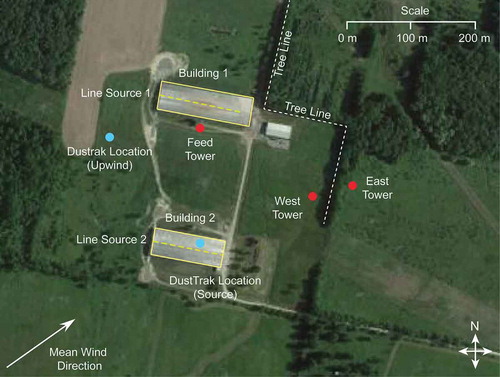
The facility consists of two buildings that acted as the main PM emission sources (Figure 2a). Each building has two mechanically ventilated manure-belt poultry pullet houses and a composting facility in between the two houses. The pullet houses in each building had air inlets on the outside walls and exhausted air toward the composting facility (Figure 2b). Air entering the compost facility was exhausted through a ridge opening on the roof peak of the building (Figure 2b). In Building 1, House 1 consists of 7 rows with about 130,000 pullets and was equipped with 25 exhaust fans, while House 2 consists of 5 rows with about 83,000 pullets with 16 exhaust fans. In Building 2, House 3 consists of 7 rows with about 116,000 pullets and was equipped with 21 exhaust fans, while House 4 consists of 6 rows with about 97,000 pullets with 17 exhaust fans. The compost house in each building was about 9 m wide. The compost windrow was turned every day and was moved 6 m every 3 days until it would exit the composting lanes after 54 days of being fully composted. The final product is dry compost from manure and can be applied as fertilizer.

Figure 2. Schematic of the Building 1 (a) top view layouts and (b) front view of the building showing the ventilation fans and the exhaust air ridge openings on top of the roof.

Measurement and instrumentation

A field measurement campaign was conducted from August 6 to 20, 2010, to obtain data on PM emissions, PM concentrations at sources and downwind locations, and meteorological conditions. The ambient PM concentration near the poultry facility was expected to be high in summer period due to the fact that the poultry facility was operated at its maximum ventilation.

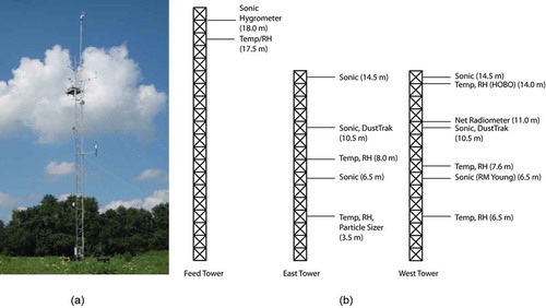
Two light towers (Figure 1) were used for placement of instruments for continuous ground-based measurements at multiple heights of 16, 10.5, and 6.5 m above ground. The towers were equipped with three-dimensional (3D) ultrasonic anemometers (CSAT3, Campbell Scientific, Inc., Logan, UT; RM81000, R.M. Young Co., Traverse City, MI) to obtain measurements of the orthogonal wind speed and sonic temperature that were required to compute the wind speed, direction, lateral and cross-wind variation, turbulence, and sensible heat flux. The anemometers have a wind speed threshold of 0.0005–0.001 m sec⁻¹. Temperature–humidity probes (HMP45C, Vaisala, Inc., Helsinki, Finland) were installed to obtain the vertical profiles of mean temperature and relative humidity. The positions of all instruments are shown in Figures 3a and 3b. The two towers were placed downwind of the PM source before and after a windbreak/vegetation barrier (East Tower and West Tower). An additional meteorological station was placed on a short mast (2 m) above a feed tower and provided observations at 18 m above the ground (Figure 1). In addition, a four-channel net radiometer (NR01, HukseFlux, Manorville, NY) was mounted on top of the East Tower to measure downward and upward short-wave and long-wave radiation and to calculate the net radiation. The “Feed-Tower” meteorological station included a 3D ultrasonic anemometer, temperature/humidity probe, and open path gas analyzer for water vapor concentrations (KH2O, Campbell Scientific, Inc., Logan, UT) for measurements of evaporation rates and latent heat flux. Data loggers were used to record the raw 10-Hz data and to calculate half-hourly statistics. Mass concentrations of PM₁₀ and PM_2.5 were measured using portable DustTrak aerosol monitors (model 8533, TSI, Inc., Shoreview, MN) mounted at 10.5 m height on both East Tower and West Tower and set to log data every 5 mins. Each DustTrak unit was zero calibrated before use. It was also custom calibrated by comparing the concentration results to the calculated concentration obtained from the weighed gravimetric PM sample on the preconditioned glass microfiber filter (37-mm GF/A catalogue number 1820037, Whatman, Pittsburgh, PA) installed inside the 37-mm filter cassette of the DustTrak unit. The filter with PM sample was also conditioned in a desiccator before the post weights were assessed. The calibration was conducted in the lab using a prototype wind-tunnel simulation chamber that was equipped with a custom-designed turntable dust feeder and isokinetic sampling tubes. All the DustTrak units used were also cross-calibrated with one another to guarantee precise measurements.

Figure 3. (a) Actual photograph of the West Tower (upwind before the tree line) with instruments installed and (b) the instruments on Feed Tower, East Tower, and West Tower and the installation heights enclosed in parentheses.

To determine the source strength of PM emissions, we conducted direct measurements of PM concentration and ventilation rates along with air temperature and relative humidity. The PM concentrations were measured using a DustTrak at the roof exhaust of Building 2. Airflow rates of three representative fans were intensively qualitified using an in situ Fans Assessment Numeration System (FANS) (Gates et al., 2004). Air temperature and relative humidity values were collocated near the DustTrak and measured using HOBO dataloggers (HOBO U23 Pro, Onset Computer Corp., Bourne, MA).

Background concentrations of PM were measured at 3 m above ground at the upwind of the buildings (Figure 1) to account for PM from other sources, such as from unpaved roads and trucks located north of the emission sources. Measurements included PM concentrations (using a DustTrak), temperature and humidity (using a HOBO sensor) and were conducted during the last 2 weeks of August 2010.

Calculation of PM emission

PM emission rates were calculated using actual airflow rate multiplied to PM concentration measurements (eq 1). The average airflow rate per fan, calculated as the mean airflow rates of the three representative fans, was multiplied to the total number of operating fans in each building to obtain the total exhaust air flow rate:

(1)

where ER is the PM emission rate (g sec⁻¹), T₀ is the temperature of exhaust air (°C), Q₀ is ventilation rate at T₀ (m³ hr⁻¹), the sum of air flows of all fans, P₀ is the atmospheric pressure of exhaust air (atm), P_atm is the standard atmospheric pressure of exhaust air (= 1 atm), is the PM concentration in exhaust air (mg m⁻³), and is the PM concentration in inlet air (mg m⁻³). The inlet PM concentration in this case was the background PM concentration obtained from the upwind location (Figure 1).

Meteorological data and topography

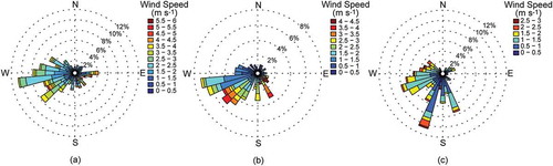
AERMET (EPA, 2004b) was the meteorological preprocessor used to calculate the PBL parameters such as the friction velocity, Monin–Obukhov length, convective velocity scale, temperature scale, mixing height, and surface heat flux (Kakosimos et al., 2011) as inputs for AERMOD. In our study, half-hourly meteorological data (wind speed and direction, ambient temperature and pressure, and cloud coverage) were obtained from the on-site tower measurements from August 8 to 14, 2010. Figure 4 shows the typical wind roses of the prevailing winds observed in the all towers during the entire study period. As observed, the typical prevailing winds with strongest intensities are southwesterly.

Figure 4. Wind roses obtained from the (a) Feed Tower (at 18 m), (b) West Tower (at 14.5 m), and (c) East Tower (at 14.5 m).

Upper air data in the Forecast Systems Laboratory (FSL) format was downloaded from the National Oceanic and Atmospheric Administration Earth System Research Laboratory (NOAA-ESRL) (Govett, 2014), recorded twice daily at Wilmington County, Wilmington, OH (Station ID: 1384), which was approximately 125 km away from the study region. Both sets of data were preprocessed in the appropriate format for AERMOD use. The site location had a relatively flat terrain and therefore AERMAP was not implemented for preprocessing.

Modeling configuration options

AERMOD View modeling package (Version 6.5.0: Lakes Environmental, 2014) was used to run AERMOD. The dispersion coefficients set were “rural” and terrain height option was set to “flat.” The pollutant type, “Other,” was specified for PM dispersion modeling. Other control options that can be set in AERMOD are the source type, release height, and emission height.

Emission sources

Source type options in AERMOD include point, area, line, and volume. The characteristics of the emission sources were summarized in Table 1. Given the layout of the building exhaust air outlets, the special line volume sources were chosen to represent the two ridge openings along the length of the building roof. The line sources were set to be elevated with adjacent configuration of the volume source. The significant parameters for this source type are the source length, source width, called “length of the side,” emission rate, and the height of the building. The width of the ridge inner opening (127 cm for Building 1 and 132 cm for Building 2) was used as the length of the side of the line source (Figure 2b).

Table 1. Summary of the source emission characteristics

Parameter	Source 1 (North Building)	Source 2 (South Building)
Source type	Line volume	Line volume
Source location	Elevated; on a building	Elevated; on a building
Base elevation (m)	342	343.6
Building height (m)	5.8	5.8
Plume width, PW (m)	1.12	1.12
Velocity at stack, vs (m sec^−1)	1.04	1.14
Surrounding wind speed, us (m sec^−1)	0.77	0.77
Average ambient temperature, Ta (K)	298.24	298.24
Temperature at stack/vent, Ts (K)	298.65	298.65

Initial release height

Air emission effective release height was computed as the sum of the physical height of the building (5.80 m) and its initial vertical dimension. Because the initial rise from the vent was not visible enough to be observed during the field campaign, the initial vertical dimension was further investigated using the well-documented sets of formulas for plume rise discussed by Anfossi (1985) and Briggs (1975).

The Briggs (1973) buoyancy flux, F_b (m⁴ sec⁻³), is a significant parameter for plume rise situations, and is equivalent to

(2)

where v_s is the stack gas exit velocity (m/sec), T_s is the stack gas temperature (K), T_a is ambient air temperature (K), ΔT = T_s – T_a, d_s is the inner diameter of the stack top (m), and g is gravitational acceleration (= 9.81 m sec⁻²). The diameter of the stack used in the equations was assumed to be the length of the side of the line source (or the width of the vent). The F_b calculated based on the data provided by Table 1 was less than 55.

For T_s ≥ T_a the crossover temperature difference (ΔT)_c was calculated to determine whether the plume rise was dominated by momentum or buoyancy (Briggs, 1973).

For F_b < 55:

(3)

and for F_b ≥ 55:

(4)

If ΔT ≥ (ΔT)_c, plume rise was assumed to be dominated by buoyancy and not by momentum. The final effective plume height was determined as follows (Briggs, 1973).

For F_b < 55:

(5)

and for F_b ≥ 55:

(6)

where h_e is the effective stack height, is the modified stack height, which was assumed to be equal to h_s without consideration of the stack tip downwash, u_s is the surrounding wind speed, and v_s is the wind speed at the stack.

When ΔT < (ΔT)_c, the plume rise is assumed to be momentum-dominated and the final plume is described by the equation

(7)

Based on the actual data collected (Table 1) at the vent of the poultry facility, the crossover temperature gradient criterion showed that the emission has no sufficient thermal buoyancy (ΔT < (ΔT)_c), and is therefore momentum-dominant. However, eq 8 was found to be applicable only when v_s/u_s is greater than 4, and in the case of this study this ratio was only estimated to be 1.36, which implies that the plume has not enough momentum to cause an initial vertical rise. The stack-tip downwash should be accounted for when 1.5, where the physical stack height has to be adjusted according to the equation

(8)

Equation 8 suggested that the release height is less than the height of the building (5.8 m), but because the release vent is close to the roof of the building, the airflow may slip through the roof surface and rise. Therefore, the release height was determined to be the same as the maximum height of the building. The virtual “stacks” assumed for CAFOs are low, and because of the presence of the roof cap on top of the vent the initial direction of the airflow is horizontal, and not the typical vertical direction observed among industrial stacks, making these established formulas for initial release height unreliable for CAFO application.

Data analysis and model performance evaluation

Measurement data for PM concentrations were analyzed using JMP 10.0 Statistical Analysis Software (SAS Institute, Inc., Cary, NC) for analysis of variance (ANOVA), t-test for paired comparisons, and Tukey–Kramer’s honest significant difference (HSD) for mean comparisons at 95% confidence interval. For the assessment of the prediction accuracy, model results were compared with direct measurements of the PM concentrations at the field. Five of the statistical parameters were used for evaluating air quality model performance (Chang and Hanna, 2004). The parameters were calculated using eqs 9–13.

(9)

(10)

(11)

(12)

(13)

where C_o is observed concentration, while and C_p is the predicted or modeled concentration.

The first two measures focused on the likelihood of the model to deviate from actual measurement values, while the last three focused on bias, as well as the scatter of the modeled results with respect to the observed ones. Criteria for model acceptability are summarized as follows (Hanna and Chang, 2012): , , , , and . These criteria were used in this study to assess the suitability of AERMOD for PM dispersion modeling from a CAFO with distributed line-source emissions.

Results and Discussion

PM concentrations and emission rates at the source

Hourly concentrations of PM₁₀ and PM_2.5 observed at the source are shown in Figure 5. The data were hourly averages of 4 days of PM concentration measurements, which are not significantly different at a 95% confidence interval. The average daily PM₁₀ and PM_2.5 concentrations were estimated to be 436.01 ± 166.77 μg m⁻³ and 291.09 ± 105.81 μg m⁻³, respectively. Strong variations were due to a significant diurnal pattern of PM concentrations. Both PM₁₀ and PM_2.5 concentrations tend to increase with bird activity as correlated to the light hours, typically from 07:00 to 19:00. The facility was also using another lighting technique called “midnight feeding” in the middle of dark hours, specifically between 00:00 to 2:00, to encourage better feed consumption of the pullets. During this period, the light was turned on to wake up the pullets, and then the feeders were run. This is why the PM concentrations during this period were high and comparable to those observed during the daytime.

Figure 5. Hourly averages of PM₁₀ and PM_2.5 concentration (in μg m⁻³) observed at the source measurement location.

The hourly average PM emission rates are shown in Figure 6. For Building 2, the average PM₁₀ and PM_2.5 were 0.067 ± 0.027 g sec⁻¹ and 0.044 ± 0.017 g sec⁻¹, respectively. For Building 1, the daily mean emission rates were calculated to be 0.073 ± 0.030 g sec⁻¹ and 0.047 ± 0.019 g sec⁻¹ for PM₁₀ and PM_2.5, respectively, based on the concentration data obtained from Building 1. There was a significant difference in both PM₁₀ [t(23) = –13.15, p < 0.001] and PM_2.5 [t(23) = –13.10, p < 0.001] emission rates from the buildings, with Building 1 having higher PM emission rates, despite having a similar number of birds in both buildings, due to the larger number of operational ventilation fans in Building 1 that was used in the PM emission calculation. Emission rates displayed a diurnal pattern and followed the same trend as the PM concentration during the day.

Figure 6. Hourly mean emission rates of PM₁₀ and PM_2.5 from Building 2 where the average PM concentration at the source was obtained.

The percentage of the PM_2.5 emission from the PM₁₀ emission at the pullet facility was about 64.71% (±0.79%). Reported PM_2.5/PM₁₀ ratio from a high-rise poultry facility with laying hens was about 7% (Lim, 2003). The variations in the observation might be due to the age of the animals and type of ventilation, as well as the location where the measurement was obtained. It was expected that at the vent this ratio will be higher, as bigger particles tend to settle out of the air stream.

PM concentrations at downwind locations

The observed PM concentrations at the West Tower and East Tower locations downwind from the source at a height of 10.5 m are illustrated in Figure 7. At the West Tower, upwind of a tree-line windbreak, the average PM₁₀ and PM_2.5 concentrations were measured to be 31.5 ± 9.1 μg m⁻³ and 29.2 ± 8.6 μg m⁻³, respectively, while at the East Tower, the average PM₁₀ and PM_2.5 concentrations were 31.9 ± 9.9 μg m⁻³ and 31.0 ± 9.7 μg m⁻³, respectively. These concentrations were not statistically different. The majority of the particles downwind of the source are PM_2.5, and no significant differences between the concentrations at the West Tower and East Tower locations were observed for both PM₁₀ [t(23) = 0.46, p = 0.65)] and PM_2.5 [t(23) = 1.84, p = 0.08] at 95% confidence interval.

Figure 7. Hourly concentrations of PM₁₀ and PM_2.5 observed at the (a) West Tower and (b) East Tower downwind of the source.

Model performance

Figure 8 shows the 1-hr and 24-hr averages of PM₁₀ and PM_2.5 concentrations observed at the West Tower and East Tower locations, plotted against the predicted 1-hr and 24-hr PM₁₀ concentrations from AERMOD. Table 2 summarizes the calculated performance indicator values of the model based on the observed data, as well as the model acceptability criteria for each measure as suggested by Chang and Hanna (2004).

Table 2. Values of statistical performance indicators for the prediction of PM concentration at West Tower and East Tower locations, downwind of the poultry facility for 1-hr and 24-hr averaging period for AERMOD simulations conducted from August 8 to 14, 2010

	PM10				PM2.5
	West Tower		East Tower		West Tower		East Tower
P	1-hr	24-hr	1-hr	24-hr	1-hr	24-hr	1-hr	24-hr	Criteria
FB	–0.11	–0.04	–0.09	–0.05	–0.11	–0.03	–0.15	–0.06	<0.03
MG	0.96	0.99	0.96	0.97	0.96	1	0.93	0.97	<1.3
NMSE	0.29	0.06	0.26	0.04	0.25	0.07	0.28	0.07	<1.5
VG	1.27	1.06	1.22	1.04	1.24	1.07	1.25	1.07	<4
FAC2	91.52%	100%	93.93	100%	93.46%	100%	94.66%	100%	>50%

Figure 8. Relationship between the measured and modeled 1-hr and 24-hr averages of PM₁₀ and PM_2.5 concentration obtained from West downwind location (a and b) and East downwind location after the windbreak (c and d). Broken lines refer to the values within the range of a factor of 2 with respect to the 1:1 values represented by the solid line. Scales are logarithmic.

Statistical comparisons show that for the simulation settings used in this study, AERMOD has met the criteria for all the statistical performance measures. FB and MG values, which account for the bias of the model in overpredicting and underpredicting, were acceptable for all simulations. This was, however, improved upon changing the averaging period from 1 hr to 24 hr. Composite measures such as NMSE, VG, and FAC2 that consider the bias and scatter of model data with respect to the observed data were also in the acceptable range. These measures were also improved upon changing the averaging period. Observed FAC2 was greater than 90%, which was more than the expected 50% criterion. The 24-hr averaging period allowed all the data to be included within the variation of FAC2.

Comparison of 1-hr concentrations

Hourly modeled and measured PM₁₀ and PM_2.5 concentrations were compared as shown in Figure 9 throughout the study period. The modeled concentrations from the West Tower and East Tower did not show significant differences. AERMOD also overpredicted concentrations for extremely low concentration scenarios, that is, when the actual PM concentrations were close to zero. Particularly, these were observed during August 12 to 13, 2010, when the background concentrations upwind were high and the prevailing wind direction was from the north. Sudden peaks in PM concentrations were observed during August 10, 2010, that caused underprediction of the model. This sudden increase could be attributed to increase in activity in the farm during this day, when composts from the compost buildings were being transported by trucks to the storage building across Building 1. Additional emissions within the vicinity of the farm were not accounted for in the model.

Figure 9. Comparison between measured and predicted 1-hr average of PM₁₀ and PM_2.5 at (a and b) West Tower and (c and d) East Tower locations, 10.5 m above the ground.

Comparison of 24-hr concentrations

Actual PM₁₀ and PM_2.5 concentrations averaged over the 24-hr period were directly compared to the modeled results as shown in Figure 10 using data from August 8, 2010, to August 14, 2010, obtained from West Tower and East Tower. The averaged results from the measurement data were compared to the NAAQS standard for both PM₁₀ and PM_2.5. Observations for PM₁₀ (Figure 10a and Figure 10c) revealed that the downwind concentrations are within the criterion of 150 μg m⁻³, while for PM_2.5, a few episodes of high concentrations above the NAAQS standard of 35 μg m⁻³ were observed (Figure 10b and Figure 10d).

Figure 10. Comparison between measured and predicted 24-hr average of PM₁₀ and PM_2.5 at (a and b) West Tower and (c and d) East Tower locations, 10.5 m above the ground. Dashed horizontal line in (b) and (d) represents the NAAQS threshold for 24-hr PM_2.5. The NAAQS threshold for PM10 (= 150 μg m⁻³) is not plotted.

PM dispersion beyond the property line

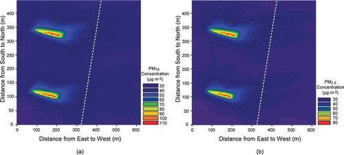
Simulations were also conducted to obtain the dispersion of PM from the poultry facilities and the PM concentrations at and beyond the property line. Figure 11 shows the dispersion of PM₁₀ and PM_2.5, respectively, from the PM sources. The values were reported as 24-hr averages obtained from running a simulation between August 8, 2010, and August 14, 2010. At the property line, the average PM₁₀ concentration was in the range of 31.77 μg m⁻³ to 34.55 μg m⁻³ and the average PM_2.5 concentration was in the range of 28.91 μg m⁻³ to 31.15 μg m⁻³. It was observed that farther downwind of the source, most of the PM was composed of PM_2.5, and PM₁₀ concentration did not significantly differ from that of PM_2.5. This result supports that PM_2.5 has a longer lifetime and higher dispersion potential in the atmosphere. Compared to the NAAQS for 24-hr mean concentrations of PM_2.5 and PM₁₀, which are reported to be 35 μg m⁻³ and 150 μg m⁻³, respectively, prediction results at the property line revealed good acceptability within the NAAQS limit, suggesting minimal levels of PM nuisance around the downwind locations surrounding the poultry facility. This comparison was only preliminary as the NAAQS requires averaging for more than 3 years of 24-hr data.

Figure 11. Dispersion of (a) PM₁₀ and (b) PM_2.5 from the source. The plot shows concentration (μg m⁻³). Broken line refers to the windbreak along the property line.

Sources of error and uncertainties

Application of AERMOD to model the dispersion of PM from CAFOs is not very well studied due to its configurations that may not resemble industrial stack sources. The prediction equations provided by AERMOD might not be very applicable to the characterization of the CAFO source. The assumption of no building downwash due to the low velocity at the PM source may affect the downwind concentrations significantly. Another source of error is the lack of actual velocity measurements at the vent, which may possibly vary within the day. The accuracy of the PM concentration measurement needs to be improved by adding correction factors for adjustment of the readings, which could be done by cross-calibrating the DustTraks with other federal reference methods. Obtaining source concentration and emission from only Building 2 may also add to errors in defining accurate emissions from Building 1. Challenge also arises on the estimation of the initial release height of the plume, which could be better verified using Lidar scan data.

Conclusion

The daily mean PM_2.5 and PM₁₀ concentrations at the exhaust of the poultry pullet buildings were measured to be 436.01 ± 166.77 μg m⁻³ and 291.09 ± 105.81 μg m⁻³, respectively, and showed a strong diurnal pattern. The corresponding PM₁₀ and PM_2.5 emission rates were 0.067 ± 0.030 g sec⁻¹ and 0.044 ± 0.019 g sec⁻¹, respectively, for Building 1, and 0.073 ± 0.030 g sec⁻¹ and 0.047 ± 0.019 g sec⁻¹, respectively, for Building 2. Results showed that the fraction of PM_2.5 emission from the pullet poultry facility was about 64.71% (±0.79%) of PM₁₀, which is high compared to typical PM emissions from poultry laying-hen facilities observed in the literature.

Application of AERMOD for PM dispersion from CAFOs is not similar to its application to industrial PM sources. In this study, specific configurations were utilized for the application of AERMOD to PM dispersion at a poultry facility, accounting for the distributed sources, unique plume rise, and strong diurnal variability of PM emission rates.

Simulation of the dispersion using AERMOD showed very good statistical agreement (FB < 0.03, MG < 1.3, NMSE < 1.5, VG < 4, and FAC2 > 50%) with observed concentrations for both PM₁₀ and PM_2.5 at two downwind locations, 10.5 m above the ground. Increasing averaging period from 1 hr to 24 hr enhanced model results, suggesting AERMOD applicability for the prediction and assessment of PM concentrations downwind of the source with respect to the NAAQS 24-hr standard for PM.

The AERMOD simulation of PM dispersion in the vicinity of the poultry facility also revealed that the PM concentrations at and beyond the downwind property line of the facilities were within NAAQS limits. In conclusion, AERMOD can be used to model the dispersion of PM from poultry facilities.

Acknowledgments

The authors acknowledge Kyle Maurer and Roderick Manuzon, former postdoctoral researchers, and students at the Ohio State University for assistance during the field campaign, as well as William Eichinger and his team, Bryson Winski, Brad Barnhardt, Sean Plenner, and Adam Thompson, from the University of Iowa.

Funding

This project was supported by the U.S. Department of Agriculture National Institute for Food & Agriculture (NIFA) Air Quality Grant CSREES-OHOR-2009-04566. WTK was funded in part by NASA Earth and Space Science Graduate Training Fellowship NNX11AL45H.

Disclaimer

Opinions expressed are those of the author and not necessarily those of the Illinois State Water Survey, the Prairie Research Institute, or the University of Illinois.

Additional information

Funding

This project was supported by the U.S. Department of Agriculture National Institute for Food & Agriculture (NIFA) Air Quality Grant CSREES-OHOR-2009-04566. WTK was funded in part by NASA Earth and Space Science Graduate Training Fellowship NNX11AL45H.

Notes on contributors

L.S. Hadlocon

L.S. Hadlocon is a postdoctoral researcher, L.Y. Zhao is an associate professor, and J. Upadhyay is a former research associate in the Department of Food, Agricultural, and Biological Engineering, at The Ohio State University, Columbus, OH.

L.Y. Zhao

L.S. Hadlocon is a postdoctoral researcher, L.Y. Zhao is an associate professor, and J. Upadhyay is a former research associate in the Department of Food, Agricultural, and Biological Engineering, at The Ohio State University, Columbus, OH.

G. Bohrer

G. Bohrer is an assistant professor, S.R. Garrity is a former postdoctoral researcher, and W. Kenny is a Ph.D. graduate student and NESSF fellow in the Department of Civil, Environmental and Geodetic Engineering at The Ohio State University, Columbus, OH.

W. Kenny

G. Bohrer is an assistant professor, S.R. Garrity is a former postdoctoral researcher, and W. Kenny is a Ph.D. graduate student and NESSF fellow in the Department of Civil, Environmental and Geodetic Engineering at The Ohio State University, Columbus, OH.

S.R. Garrity

G. Bohrer is an assistant professor, S.R. Garrity is a former postdoctoral researcher, and W. Kenny is a Ph.D. graduate student and NESSF fellow in the Department of Civil, Environmental and Geodetic Engineering at The Ohio State University, Columbus, OH.

J. Wang

J. Wang is an atmospheric scientist in the Center of Atmospheric Sciences at University of Illinois at Urbana-Champaign, Champaign, IL.

B. Wyslouzil

B. Wyslouzil is a professor in the Department of Chemical and Biomolecular Engineering at The Ohio State University, Columbus, OH.

J. Upadhyay

L.S. Hadlocon is a postdoctoral researcher, L.Y. Zhao is an associate professor, and J. Upadhyay is a former research associate in the Department of Food, Agricultural, and Biological Engineering, at The Ohio State University, Columbus, OH.

References

- Anfossi, D. 1985. Analysis of plume rise data from five TVA steam plants. J. Clim. Appl. Meteorol. 24:1225–36. doi:10.1175/1520-0450(1985)024<1225:AOPRDF>2.0.CO;2
- Aylor, D.E., and T.K. Flesch. 2001. Estimating spore release rates using a Lagrangian stochastic simulation model. J. Appl. Meteorol. 40(7):1196–208. doi:10.1175/1520-0450(2001)040<1196:ESRRUA>2.0.CO;2
- Bohrer, G., G.G. Katul, R. Nathan, R.L. Walko, and R. Avissar. 2008. Effects of canopy heterogeneity, seed abscission and inertia on wind-driven dispersal kernels of tree seeds. J. Ecol. 96(4):569–80. doi:10.1111/j.1365-2745
- Bonifacio, H.F., R.G. Maghirang, E.B. Razote, S.L. Trabue, and J.H. Prueger. 2013. Comparison of AERMOD and WindTrax dispersion models in determining PM10 emission rates from a beef cattle feedlot. J. Air Waste Manage. Assoc. 63(5):545–46. doi:10.1080/10962247.2013.768311
- Briggs, G.A. 1973. Diffusion estimation for small emissions. http://www.osti.gov/energycitations/product.biblio.jsp?osti_id=5118833 (accessed July 23, 2013).
- Briggs, G. A. 1975. Plume rise from multiple sources. http://www.osti.gov/energycitations/product.biblio.jsp?osti_id=4164190 (accessed July 23, 2013).
- Britter, R.E., and S.R. Hanna. 2003. Flow and dispersion in urban areas. Annu. Rev. Fluid Mech. 35(1):469–96. doi:10.1146/annurev.fluid.35.101101.161147
- Cheung, H.C., T. Wang, K. Baumann, and H. Guo. 2005. Influence of regional pollution outflow on the concentrations of fine particulate matter and visibility in the coastal area of southern China. Atmos. Environ. 3(34):6463–74. doi:10.1016/j.atmosenv.2005.07.033
- Cimorelli, A.J., S.G. Perry, A. Venkatram, J.C. Weil, R.J. Paine, R.B. Wilson, R.F. Lee, W.D. Peters, and R.W. Brode. 2005. AERMOD: A dispersion model for industrial source applications. Part I: General model formulation and boundary layer characterization. J. Appl. Meteorol. 44(5): 682–93. doi:10.1175/JAM2227.1
- Vieira de Melo, A.M., J.M. Santos, I. Mavroidis, and N.C. Reis, Jr. 2012. Modelling of odour dispersion around a pig farm building complex using AERMOD and CALPUFF: Comparison with wind tunnel results. Build. Environ. 56: 8–20. doi:10.1016/j.buildenv.2012.02.017
- Damschen, E.I., D.V. Baker, G. Bohrer, R. Nathan, J.L. Orrock, J.R. Turner, L.A. Brudvig, N.M. Haddad, D.J. Levey, and J.J. Tewksbury. 2014. How fragmentation and corridors affect wind dynamics and seed dispersal in open habitats. Proc. Natl. Acad. Sci. USA 111(9): 3484–89. doi:10.1073/pnas.1308968111
- Dresser, A.L., and R.D. Huizer. 2011. CALPUFF and AERMOD model validation study in the near field: Martins Creek revisited. J. Air Waste Manage. Assoc. 61(6): 647–59. doi:10.3155/1047-3289.61.6.647
- Douwes, J., P. Thorne, N. Pearce, and D. Heederik. 2003. Bioaerosol health effects and exposure assessment: Progress and prospects. Ann. Occup. Hyg. 47(3):187–200. doi:10.1093/annhyg/meg032
- Environmental PublicWorks. 2004. The Clean Air Act. http://www.epw.senate.gov/envlaws/cleanair.pdf (accessed July 23, 2013).
- Gates, R. S., K.D. Casey, H. Xin, E.F. Wheeler, and J.D. Simmons. 2004. Fan Assessment Numeration System (FANS) design and calibration specifications. Trans. ASABE 47(5):1709–15. doi:10.13031/2013.17613
- Govett, M. W. 2014. NOAA/ESRL radiosonde database. http://www.esrl.noaa.gov/raobs1 (accessed July 23, 2013).
- Hanna, S.R., and J. Chang. 2012. Air Pollution Modeling and Its Application XXI, ed. D. G Steyn and S. T. Castelli. Dordrecht, The Netherlands: Springer Netherlands.
- Holmes, N.S., and L. Morawska. 2006. A review dispersion modelling and its application to the dispersion of particles: An overview of different dispersion models available. Atmos. Environ. 40(30): 5902–28. doi:10.1016/j.atmosenv.2006.06.003
- Kakosimos, K.E., M.J. Assael, and A.S. Katsarou. 2011. Application and evaluation of AERMOD on the assessment of particulate matter pollution caused by industrial activities in the Greater Thessaloniki Area. Environ. Technol. 32(6): 593–608. doi:10.1080/09593330.2010.506491
- Kirkhorn, S.R., and V.F. Garry. 2000. Agricultural lung diseases. Environ. Health Perspect. 108:705–12. doi:10.2307/3454407
- Lakes Environmental. 2014. US EPA models: Air quality models, documentation, & guidelines. http://www.weblakes.com/download/us_epa.html (accessed July 23, 2013).
- Mavroidis, I., R. Griffiths, and D. Hall. 2003. Field and wind tunnel investigations of plume dispersion around single surface obstacles. Atmos. Environ. 37(21):2903–18. doi:10.1016/S1352-2310(03)00300-5
- Merchant, J.A., A.L. Naleway, E.R. Svendsen, K.M. Kelly, L.F. Burmeister, A.M. Stromquist, and E.A. Chrischilles. 2005. Asthma and farm exposures in a cohort of rural Iowa children. Environ. Health Perspect. 113(3):350–56. doi:10.1289/ehp.7240
- Minnesota Pollution Control Agency. 2003. Draft environmental impact statement on the Hancock Pro Pork Feedlot project, Stevens and Pope counties. http://www.eqb.state.mn.us/pdf/FileRegister/hancock_drafteis.pdf (accessed July 23, 2013).
- O’Shaughnessy, P.T., and R. Altmaier. 2011. Use of AERMOD to determine a hydrogen sulfide emission factor for swine operations by inverse modeling. Atmos. Environ. 45(27):4617–25. doi:10.1016/j.atmosenv.2011.05.061
- Sun, Y., G. Zhuang, A. Tang, Y. Wang, and Z. An. 2006. Chemical characteristics of PM2.5 and PM10 in haze—Fog episodes in Beijing. Environ. Sci. Technol. 40(10):3148–55. doi:10.1021/es051533g
- U.S. Environmental Protection Agency. 2004a. National emission inventory—Ammonia emissions from animal husbandry operations. http://www.epa.gov/ttnchie1/ap42/ch09/related/nh3inventorydraft_jan2004.pdf (accessed July 23, 2013).
- U.S. Environmental Protection Agency. 2004b. User’s guide for the AMS/EPA regulatory model—AERMOD. http://www.epa.gov/scram001/7thconf/aermod/aermodugb.pdf (accessed July 23, 2013).
- Vallamsundar, S., and J. Lin. 2012. MOVES and AERMOD used for PM2.5 conformity hot spot air quality modeling. Transport. Res. Rec. 2270:39–48. doi:10.3141/2270-06
- Wang, J., A.L. Hiscox, D.R. Miller, T.H. Meyer, and T.W. Sammis. 2008. A dynamic Lagrangian, field-scale model of dust dispersion from agriculture tilling operations. Trans. ASABE 51(5):1763–74. doi:10.13031/2013.25310
- Weil, J.C., P.P. Sullivan, E.G. Patton, and C.H. Moeng. 2012. Statistical variability of dispersion in the convective boundary layer: Ensembles of simulations and observations. Boundary-Layer Meteorol. 145(1): 185–210. doi:10.1007/s10546-012-9704-y
- Willis, G.E., and J.W. Deardorff. 1981. A laboratory study of dispersion from a source in the middle of the convectively mixed layer. Atmos. Environ. 15(2): 109–17. doi:10.1016/0004-6981(81)90001-9