Derivation of exemption formulas for air quality regulatory applications

Abstract

The regulatory agencies and the industries have the responsibility for assessing the environmental impact from the release of air pollutants, and for protecting environment and public health. The simple exemption formula is often used as a criterion for the purpose of screening air pollutants. That is, the exemption formula is used for air quality review and to determine whether a facility applying for and described in a new, modified, or revised air quality plan is exempted from further air quality review. The Bureau of Ocean Energy Management’s (BOEM) air quality regulations are used to regulate air emissions and air pollutants released from the oil and gas facilities in the Gulf of Mexico. If a facility is not exempt after completing the air quality review, a refined air quality modeling will be required to regulate the air pollutants. However, at present, the scientific basis for BOEM’s exemption formula is not available to the author. Therefore, the purpose of this paper is to provide the theoretical framework and justification for the use of BOEM’s exemption formula. In this paper, several exemption formulas have been derived from the Gaussian and non-Gaussian dispersion models; the Gaussian dispersion model is a special case of non-Gaussian dispersion model. The dispersion parameters obtained from the tracer experiments in the Gulf of Mexico are used in the dispersion models. In this paper, the dispersion parameters used in the dispersion models are also derived from the Monin-Obukhov similarity theory. In particular, it has been shown that the total amount of emissions from the facility for each air pollutant calculated using BOEM’s exemption formula is conservative.

Implications: The operation of offshore oil and gas facilities under BOEM’s jurisdiction is required to comply with the BOEM’s regulations. BOEM’s air quality regulations are used to regulate air emissions and air pollutants released from the oil and gas facilities in the Gulf of Mexico. The exemption formulas have been used by BOEM and other regulatory agencies as a screening tool to regulate air emissions emitted from the oil and gas and other industries. Because of the BOEM’s regulatory responsibility, it is important to establish the scientific basis and provide the justification for the exemption formulas. The methodology developed here could also be adopted and used by other regulatory agencies.

Introduction

The Department of the Interior Bureau of Ocean Energy Management (BOEM) has regulatory responsibility for assessing air quality impacts that may result from oil and gas exploration and development in the Gulf of Mexico Outer Continental Shelf (OCS) Region. BOEM’s air quality regulations (30 CFR 550 subparts B and C) pertain to assessing and controlling OCS emissions and to regulating air pollution. To regulate the emissions of air pollutants from oil and gas activities, BOEM uses an exemption formula to estimate the annual total amount of air emissions, the so-called “exemption level,” which is used for screening purposes. If OCS emission sources exceed this threshold value, the lessee is required to perform further air quality modeling and may be required to control emissions at the source or to reduce emissions at another facility affecting the same onshore area that is affected by the source at issue.

BOEM’s exemption formula for total suspended particulates, sulfur dioxide, nitrogen oxides, and volatile organic compounds is

(1)

which is a relationship between the total exemption amount of air emissions for each air pollutant, in tons/year (E), and the distance to shore, in statute miles (D), as given in 30 CFR 550.303. The justification of this exemption formula is not set out in 30 CFR 550.303; the scientific basis for this exemption formula is not available to the author of this paper. Therefore, the purpose of this paper is to provide the theoretical framework, derive diffusion models, and verify BOEM’s exemption formula. In this paper, I have derived several simple exemption formulas, the generalization of BOEM’s exemption formula. For regulatory applications and the purpose of screening the total allowable amount of air emissions released from OCS sources, it is desirable to use a simple exemption formula.

Diffusion Models

The purpose of this paper is to derive exemption formulas, in particular to investigate BOEM’s exemption formula, and to provide the theoretical framework for the exemption formula, eq 1, using the traditional Gaussian, non-Gaussian diffusion, and the Offshore and Coastal Dispersion (OCD) models. The experimental data collected over water are also used in the air quality models. It will be shown that the Gaussian diffusion model is a special case of the non-Gaussian diffusion model; therefore, the non-Gaussian diffusion model is more robust than and superior to the traditional Gaussian diffusion model.

The diffusion parameters (also called dispersion parameters) associated with the diffusion models can be obtained from the experimental data or the atmospheric surface boundary theory, the so-called the Monin-Obukov similarity theory.

The diffusion models and the associated diffusion parameters are derived in the following sections.

Gaussian diffusion model

A complete and popular form of the Gaussian diffusion model can be written as

(2)

where c is the concentration of an air pollutant (μg/m³); (x, y, z) is the coordinate system of a point; Q is the emission rate in μg/sec; h is the effective stack height; u is the mean wind speed (m/sec), a constant value; σ_y is the lateral, horizontal standard deviation of a plume, representing the plume width (m); and σ_z is the vertical standard deviation of a plume, representing the a plume thickness (m). When the emission source is released at the ground level (h = 0), at a ground-level receptor (y = 0 and z = 0), the above equation, eq 2, becomes eq 3, below.

The traditional Gaussian diffusion model for the ground-level centerline concentrations and for a source released at the ground level can be written as (see Gifford, 1960)

(3)

where c is the ground-level centerline concentration of an air pollutant (μg/m³) and Q is the emission rate in μg/sec from a ground-level source. Equation 3 also can be rewritten as

(4)

Equation 3 is the source and receptor relationship, which indicates that the air concentration, c, at a receptor located at the ground level at a downwind distance depends on the emission rate, Q, the mean wind speed, u, and the horizontal and vertical standard deviations of a plume, σ_y and σ_z, respectively. The standard deviations of a plume can be represented as a function of downwind distance by power exponents (see Case Study for Exemption Formulas). Equation 4 is the inverse relation of eq 3, that is, for a specific value of air concentration at the receptor location downwind from a source, the emission rate Q in eq 4 can be considered as the threshold value for the air emissions, that is, the maximum allowable amount of air emissions released from an OCS source.

Plume in the well-mixed layer

The plume trapped in the well-mixed atmospheric boundary layer is considered here. When the atmosphere is adiabatic in the neutral stability class D, under this condition (by definition), there is no inversion mixing lid in the atmospheric boundary layer. Nevertheless, let us consider the air concentration in a well-mixed layer. After the plume interacts with the mixing lid, it still takes quite some time for the concentration of a plume to become uniformly well mixed in the vertical in the presence of an inversion layer.

The simplified equation for the ground-level centerline concentration, c_zi, with an inversion lid in the well-mixed atmospheric boundary layer can be expressed as (see Arya, 1999)

(5)

where z_i is the mixing height. From eqs 4 and 5, we obtain

(6)

Let us further consider the air concentration at a ground-level receptor at the downwind distance of 10 km, the plume width, σ_z, is about 100 m for the neutral atmospheric stability class D, whereas the mixing depth on the average is about 500–1000 m or higher. That is, the plume height (width) is still far less than the mixing height by a factor of more than 5. Setting the mixing height z_i = 500 m, from eq 6, we have

(7)

Equation 7 indicates that at a downwind distance of 10 km, the Gaussian diffusion model still predicts much higher air concentration than that of the well-mixed diffusion model, that is, the predicted air concentration using the Gaussian diffusion model is still conservative as it compares with the well-mixed diffusion model at a downwind distance of 10 km.

Non-Gaussian diffusion model

On the basis of the principle of mass conservation, the equation of steady-state diffusion from an elevated point source in a turbulent shear flow may be written as (Huang, 1979; also see Seinfeld and Pandis, 1998; Arya, 1999)

(8)

where K_y is the lateral, horizontal eddy diffusivity and K_z is the vertical eddy diffusivity. The wind speed and the vertical and lateral diffusivities are expressed as

(9)

(10)

and

(11)

by virtue of Taylor’s hypotheses (Taylor, 1921).

Methods for estimating the diffusion parameters, a, b, p, and n, are derived in the next section of the paper. The diffusion parameters associated with the vertical eddy diffusivity, K_z, can be obtained from the Monin-Obukhov similarity theory, which is described in the section Estimation of Parameters.

Using eqs 9, 10, and 11, the solution of eq 8 for an elevated point source is (Huang, 1979; also see Seinfeld and Pandis, 1998; Arya, 1999)

(12)

where α = 2 + p − n; ν = (1 − n)/α; I_−ν is the modified Bessel function of the first kind of order −ν; and the point source is situated at a location (0, y_s, z_s); z is the receptor height. The non-Gaussian diffusion eq 12 is a general equation; the traditional diffusion equation or eq 4 is a special case of eq 12. Equation 12 is a more general solution and it reduces to the Gaussian form for p = n = 0; and for a point source near the ground, eq 12 reduces to the exponential form (Huang, 1979) and also to the exponential form for p = 0, n = 1, and b = ku_*, where k is von Karman constant and u_* is the friction velocity (also see Arya, 1999).

For a point source released at the ground level, that is, at a point at (y_s = 0, z_s = 0), eq 12 reduces to

(13)

where

(14)

where and is the gamma function.

The diffusion models derived in this section are used for the calculation of the hourly air pollution concentration.

Estimation of Parameters: a, b, p, and n

The non-Gaussian diffusion eq 12 or 13 is quite general, and robust, and the parameters in eqs 9 and 10 or in eq 12 can be estimated from the well-established surface similarity theory, the Monin-Obukov similarity theory, and meteorological conditions (see Huang, 1979; Seinfeld and Pandis, 1998; Arya, 1999).

According to the Monin-Obukhov similarity theory (Monin and Obukhov, 1954), the nondimensional wind shear can be expressed as

(15)

where k is the von Karman constant and is equal to 0.4, u_* is the friction velocity, and L is the Monin-Obukhov stability length. And in eq 15 is the nondimensional wind shear, defined below.

In eq 15, the Businger-Dyer formula of the nondimensional wind shear for unstable atmospheric condition can be expressed as (Dyer, 1974)

(16)

where γ = 16 (see Dyer, 1974).

For stable condition, the nondimensional wind shear is given by Webb (1970) as

(17)

Integrating eq 15 with respect to height z, we obtain the nondimensional wind profile as (see Huang, 1979)

(18)

where z_o is the surface roughness and

(19)

From eqs 9, 15, and 18, we obtain the power index p in eq 9 as

(20)

Once the power index p is known, the parameter “a” in eq 9 at a fixed height can be estimated as

(21)

According to the Monin-Obukhov similarity theory, the eddy diffusivity for momentum can be expressed as

(22)

Differentiating eq 10 with respect to the height, we obtain

(23)

Using eq 22, from eq 23 we obtain the power index n as

(24)

for unstable

for neutral

for stable

With the known value of the index n, we can obtain the parameter b from eq 10 as

(25)

Therefore, we can estimate the parameters a, b, p, and n from eqs 21, 25, 20, and 24, respectively.

Case Study for Exemption Formulas

The diffusion models are used to derive the exemption formulas in this section. Four cases of diffusion models or exemption formulas are investigated in this study. They are as follows:

• Case 1. Diffusion formula and exemption formula derived using the Gaussian model (Gifford, 1960) and the Smith diffusion formula for the horizontal standard deviation, σ_y (Smith, 1968), and the Smith diffusion formula for the vertical standard deviation, σ_z (Smith, 1972).

  Case 2. Diffusion formula and exemption formula derived using the non-Gaussian diffusion model (Huang, 1979) and the Smith diffusion formula of horizontal standard deviation, σ_y (Smith, 1968).

  Case 3. Diffusion formula and exemption formula derived using Gaussian diffusion model (Gifford, 1960) and the Smith diffusion formula for the vertical standard deviation, σ_z (Smith, 1972), and the horizontal standard deviation, σ_y, over water (Dabberdt et al., 1982).

  Case 4: The OCD model (DiCristofaro and Hanna, 1989) is used when total amount of air emissions exceeds the exemption level. The OCD model is a BOEM-approved diffusion model. The model adopts the Draxler horizontal standard deviation, σ_y, (Draxler, 1976) and the Briggs vertical standard deviation, σ_z (Briggs, 1973).

The available over-water data (see Dabberdt et at., 1982 and DiCristofaro and Hanna, 1989) are also used in the modeling. The case studies for these cases and the derivation of the exemption formulas are described in the following sections.

Gaussian diffusion model

The standard deviations of a plume, σ_y and σ_z, can be represented as a power law by fitting the experimental data as

(26)

(27)

The standard deviations of a plume depend on the atmospheric stability, the meteorological conditions, and the downwind distance. Through the use of eqs 26 and 27, the traditional Gaussian equation, eq 3, becomes

(28)

Therefore, the total allowable amount of air emissions for the exemption threshold value can be determined at a source location once the air pollution concentration, c, at a receptor location, the mean wind speed, u, and the downwind distance x with the exponent b_y + b_z are specified, where a_y, a_z, b_y, and b_z are diffusion parameters depending on the meteorological conditions.

If we set

(29)

and

(30)

then eq 28 reduces to BOEM’s exemption formula, eq 1. Thus, eq 28 is the generalization of BOEM’s exemption formula, eq 1. In general and in the real atmosphere, b_y + b_z (≠ 1) is not equal to 1 (see Table 1).

Table 1. The diffusion formulas recommended by various authors

Case	Author	ay	by	az	bz	E (tons/yr)
	BOEM Exemptionformula					33.3D
1	M.E. Smith (1968): σy F.B. Smith (1972): σz	0.32	0.78	0.199 (m)	0.76	27.4D^1.54
2	C.H. Huang (1979): Non-Gaussian model M.E. Smith (1968): σy	0.32	0.78		β = 1	16.7D^1.78
3	SRI (1982): σy over water F.B. Smith (1972): σz	0.0933	0.936	0.199 (m)	0.76	25.26D^1.70
4	OCD model* Draxler (1976): σy Briggs (1973): σz	—	—	—	—	—

Notes: The stability class is D and the wind speed is set at 5 m/sec, where E is emission rate in tons/year and D is the distance to shore in statute miles. The diffusion formulas correspond to open rural areas, and some data are obtained over water. *The OCD model is a Gaussian diffusion model. Here I use the Briggs (1973) formula for the vertical standard deviation of a plume and the Draxler (1976) formula for the horizontal standard deviation for a plume.

For the neutral stability class D, the lateral diffusion parameter, σ_y, can be expressed as (Smith, 1968)

(31)

where x is in meters. And the vertical diffusion parameter σ_z is given by Smith (1972) as

(32)

where both σ_z and x are in kilometers. Equation 32 can be converted into the following equation:

(33)

where x is in meters.

The diffusion formulas and parameters recommended by Smith (1968) and Smith (1972), and those used in the OCD model, are summarized in Table 1. The lateral diffusion parameter, σ_y, obtained from the tracer experiment over water (Dabberdt et al., 1982), is also given in Table 1.

If we set the wind speed, u = 5 m/sec, and the air pollution concentration, c = 1 μg/m³ (the modeling Significant Impact Levels, SILs, for annual average nitrogen oxides [NO_x], sulfur oxides [SO_x], volatile organic compounds [VOCs], and total suspended particulates [TSP; particulates PM₁₀]) for the neutral stability class D, then eq 28 becomes

(34)

(35)

Equation 35 is equivalent to

(36)

for case 1.

In general, the relationship between the total exemption amount of air emissions and the distance to shore used in the BOEM air quality review depends on atmospheric conditions, wind speed, and the air pollution concentration specified at a receptor location.

Non-Gaussian diffusion model

Using the lateral diffusion parameter, σ_y, from eq 26, the non-Gaussian diffusion equation, eq 13, becomes

(37)

In the above equation, it is shown that for a specific (predetermined) value of air concentration at a receptor, the total allowable amount of air emissions released from a ground-level source depends on the downwind distance with a power exponent of b_y+β.

For the stability class D, we have a_y = 0.32, b_y = 0.78 from Smith (1968). The exemption formula given in eq 1 was provided at the time when most diffusion experiments were conducted in the open rural country (see Briggs, 1973). From the Monin-Obukhov similarity theory, we obtain a = 3.24, p = 0.189, b = 0.151, n = 1, β =1, and A = 5.57. The OCD model is also used to investigate the dispersion of air emissions over water.

Therefore, eq 37 becomes

(38)

which is equivalent to

(39)

for case 2 (non-Gaussian diffusion model).

From eq 34, we have

(40)

for case 3 (Gaussian diffusion model with tracer data).

The Gaussian diffusion model, where the mean wind speed and the vertical eddy diffusivity are uniform and independent of height, is a special case of the non-Gaussian diffusion model (Huang, 1979); therefore, the non-Gaussian diffusion model is more robust than and superior to the traditional Gaussian diffusion model. That is, the diffusion formula derived from the non-Gaussian diffusion model, eq 37, is more general than that derived from the Gaussian diffusion model, eq 34.

The diffusion formulas derived from the Gaussian and non-Gaussian diffusion models for cases 1, 2, and 3, respectively, are presented in Table 1 and plotted in Figure 1.

Figure 1. Comparison of three different diffusion formulas. Set c = 1 μg/m³ and u = 5/sec. (1) Case 1: Diffusion formula obtained from the Gaussian model. (2) Case 2: Diffusion formula obtained from the non-Gaussian model. (3) Case 3: Diffusion formula obtained from the tracer experimental data.

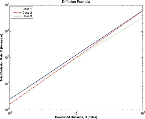
The comparison of various diffusion formulas is given in Figure 1. If we set E = time Q, where time is equal to 1 hr, then these diffusion formulas also can be used as the exemption formulas for 1-hr air emissions when the atmospheric stability F is used for the worst-case scenario or a certain value of air concentration is specified.

The annual emission exemption amount for air pollutants is described in the next section.

Exemption Formulas for Annual Emissions

BOEM’s exemption formula, eq 1, is a relationship between the annual total allowable amount of air emissions and the distance to shore, it is expressed as

(41)

where E is the annual total amount of emissions, the emission rate in tons/yr; and D is distance to shore from the pollutant source in statute miles.

The BOEM air quality review is conducted in accordance with 30 CFR 550.303 regulations, which also regulate air pollutants. The formula in eq 1 or eq 41 is used to screen the annual exemption amount of air emissions to determine if the annual exemption amount of air emissions released from the OCS water is in compliance with the regulations. If the total annual amount of air missions is not exempt from under the air quality review, the next step is to determine whether the air emissions released from the OCS sources is in compliance with Significant Impact Level and the National Ambient Air Quality Standards (NAAQS). Equation 4 is for the calculation of the hourly air pollutant concentration at a receptor location, and it is expressed as

(42)

Using eq 42, the annual air pollution concentration at a receptor location can be written as

(43)

or

(44)

where is the annual mean air concentration, f(θ) is the frequency of the wind blowing into the sector associated with the receptor (only a fraction of wind blowing into this sector that includes the receptor, that is, to take into account of wind directions in eq 43), and Q₀ is a constant emission rate.

Let us set the wind blowing in the direction of the receptor at 10% of the total time, that is, we have f(θ) = 0.1. Then, we have

(45)

Similarly using eqs 28 through 40, we have

(46)

for case 1 (traditional Gaussian diffusion model);

(47)

for case 2 (non-Gaussian diffusion model); and

(48)

for case 3 (Gaussian diffusion model with over-water tracer data).

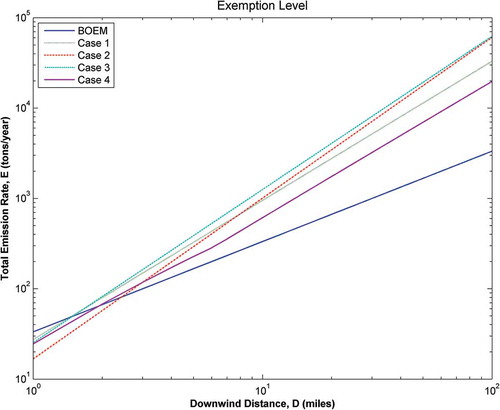
The total allowable air emissions for these cases are plotted in Figure 2. The results obtained from the OCD model (case 4) are also plotted in Figure 2.

Figure 2. Comparison of five different exemption formulas. Set c = 1 μg/m³ and u = 5 m/sec. (1) BOEM’s exemption formula. (2) Case 1. Diffusion formula and exemption formula derived using the Gaussian model (Gifford, 1960) and the Smith diffusion formula for the horizontal standard deviation, σ_y (Smith, 1968), and the Smith diffusion formula for the vertical standard deviation, σ_z (Smith, 1972). (3) Case 2. Diffusion formula and exemption formula derived using the non-Gaussian diffusion model (Huang, 1979) and the Smith diffusion formula of horizontal standard deviation, σ_y (Smith, 1968). (4) Case 3. Diffusion formula and exemption formula derived using Gaussian diffusion model (Gifford, 1960) and the Smith diffusion formula for the vertical standard deviation, σ_z (Smith, 1972), and the horizontal standard deviation, σ_y, over water (Dabberdt et al., 1982). (5) Case 4: The OCD model (DiCristofaro and Hanna, 1989) is used when total amount of air emissions exceeds the exemption level. The OCD model is a BOEM-approved diffusion model. The model adopts the Draxler horizontal standard deviation, σ_y (Draxler, 1976), and the Briggs vertical standard deviation, σ_z (Briggs, 1973).

Conclusion

In this study, we provide the theoretical basis and framework for the derivation of simple dispersion models and the exemption formulas. BOEM’s exemption formula is a screening formula, which has been used for the regulatory applications; it is used to regulate the air emissions emitted from oil and gas facilities in the Gulf of Mexico. According to BOEM’s regulations, if the total amount of air emissions from an oil and gas facility exceeds the exemption level, the lessee needs to use a BOEM-approved air quality model, such as the OCD model, to demonstrate that the results obtained from the air quality model are in compliance with BOEM’s air quality regulations and National Ambient Air Quality Standards (NAAQS).

Several simple diffusion models and exemption formulas have been derived in this paper. BOEM’s exemption formula (E = 33.3 D) is examined in light of the traditional Gaussian, non-Gaussian dispersion, and OCD models; the parameters in the non-Gaussian dispersion model are obtained from the atmospheric boundary layer theory.

In this paper, we set the stability class D and use the diffusion parameters of the lateral standard deviations (Smith, 1968; Draxler, 1976), the vertical standard deviations (Smith, 1973; Briggs, 1973) for the open rural areas, and the available over-water data. Based on these conditions, we have derived several exemption formulas for air quality review. And if a facility is not exempt after completing the air quality review, the next step is to conduct air quality modeling to determine if the total annual amount of air emissions is in compliance with the annual air quality standards for nitrogen dioxide, sulfur dioxide, total particulates, and volatile organic compounds. In the Gulf of Mexico, the atmospheric conditions overall are slightly unstable. In general, the annual total exemption amount of air emissions is a power function of distance rather than only the distance. Thus, the diffusion models derived in this study are the generalization of BOEM’s exemption formula. The comparison of BOEM’s exemption formula with several newly derived diffusion formulas shows that the annual total amount of air emissions calculated from BOEM’s exemption formula is conservative. Furthermore, the non-Gaussian diffusion model is more robust than and superior to the traditional Gaussian dispersion model, because the Gaussian diffusion model is a special case of the non-Gaussian diffusion model. The theoretical derived formulas in this paper are more robust and hence preferable.

Funding

The author also appreciates the support of the U.S. Department of the Interior, Bureau of Ocean Energy Management, Gulf of Mexico OCS Region, during the preparation of the manuscript. The opinions expressed by the author are his own and do not necessary reflect the opinion of the U.S. Government.

Acknowledgment

The author thanks and appreciates the anonymous reviewers for their comments and suggestions on the manuscript, which resulted in substantial improvement of the paper.

Additional information

Notes on contributors

C.H. Huang

C.H. Huang is a certified consulting meterorologist in the Physical/Chemical Sciences Section at the Bureau of Ocean Energy Management, Gulf of Mexico OCS Region, the Department of the Interior, New Orleans, LA.

References

- Arya, P.S. 1999. Air Pollution Meteorology and Dispersion. New York: Oxford University Press.
- Briggs, G.A. 1973. Diffusion Estimations for Small Emissions. Atmospheric Turbulence and Diffusion Laboratory Contribution 79. Oak Ridge, TN: Atmospheric Turbulence and Diffusion Laboratory.
- Dabberdt, W.F., R. Brodzinsky, B. Cantrell, and R.E. Ruff. 1982. Atmospheric Dispersion over Water and in the Shoreline Transition Zone. Final Report 3450. Meno Park, CA: SRI International.
- DiCristofaro, D.C., and S.R. Hanna. 1989. The Offshore and Coastal Dispersion Model. Volume I, User’s Guide. Contract No. 14-12-001-30396. Washington, DC: Mineral Management Service, U.S. Department of the Interior.
- Draxler, R.R. 1976. Determination of atmospheric diffusion parameters. Atmos. Environ. 10:99–105. doi:10.1016/0004-6981(76)90226-2
- Dyer, A.J. 1974. A review of flux-profile relationships. Boundary Layer Meteorol. 7:168–178. doi:10.1007/BF00240838
- Gifford, F.A. 1960. Atmospheric dispersion calculations using the generalized Gaussian plume model. Nucl. Saf. 2: 56–59, 67–68.
- Huang, C.H. 1979. A theory of dispersion in turbulent shear flow. Atmos. Environ. 13:453–463. doi:10.1016/0004-6981(79)90139-2
- Monin, A.A., and A.M. Obukhov. 1954. Basic regularity in turbulence mixing in the surface layer of the atmosphere. Trud. Geofiz. Inst. Akad. Nak. SSSR 24:163–187.
- Seinfeld, J.H., and S.N. Pandis. 1998. Atmospheric Chemistry and Physics: From Air Pollution to Climate Change. New York: John Wiley & Sons.
- Smith, F.B. 1972. A scheme for estimating the vertical dispersion of a plume from a source near ground level. In Proceedings of the Third Meeting of the Expert Panel on Air Quality Modeling, Paris, France, October 2–3, Chapter 17. NATO-CCMS-14. Brussels: NATO.
- Smith, M.E. 1968. Recommended Guide for the Prediction of the Dispersion of Airborne Effluents, 1st ed. New York: American Society of Mechanical Engineers.
- Taylor, G.I. 1921. Diffusion by continuous movement. Proc. London Math. Soc. 2:196–211.
- Webb, E.K. 1970. Profile relationship: The log-linear range and extension to strong stability. Q. J. R. Meteol. Soc. 96:67–90. doi:10.1002/qj.49709640708