Accuracy of vertical radial plume mapping technique in measuring lagoon gas emissions

Abstract

Recently, the U.S. Environmental Protection Agency (EPA) posted a ground-based optical remote sensing method on its Web site called Other Test Method (OTM) 10 for measuring fugitive gas emission flux from area sources such as closed landfills. The OTM 10 utilizes the vertical radial plume mapping (VRPM) technique to calculate fugitive gas emission mass rates based on measured wind speed profiles and path-integrated gas concentrations (PICs). This study evaluates the accuracy of the VRPM technique in measuring gas emission from animal waste treatment lagoons. A field trial was designed to evaluate the accuracy of the VRPM technique. Control releases of methane (CH₄) were made from a 45 m × 45 m floating perforated pipe network located on an irrigation pond that resembled typical treatment lagoon environments. The accuracy of the VRPM technique was expressed by the ratio of the calculated emission rates (Q_VRPM) to actual emission rates (Q). Under an ideal condition of having mean wind directions mostly normal to a downwind vertical plane, the average VRPM accuracy was 0.77 ± 0.32. However, when mean wind direction was mostly not normal to the downwind vertical plane, the emission plume was not adequately captured resulting in lower accuracies. The accuracies of these nonideal wind conditions could be significantly improved if we relaxed the VRPM wind direction criteria and combined the emission rates determined from two adjacent downwind vertical planes surrounding the lagoon. With this modification, the VRPM accuracy improved to 0.97 ± 0.44, whereas the number of valid data sets also increased from 113 to 186.

Implications: The need for developing accurate and feasible measuring techniques for fugitive gas emission from animal waste lagoons is vital for livestock gas inventories and implementation of mitigation strategies. This field lagoon gas emission study demonstrated that the EPA’s vertical radial plume mapping (VRPM) technique can be used to accurately measure lagoon gas emission with two downwind vertical concentration planes surrounding the lagoon.

Introduction

Anaerobic treatment lagoons and storage ponds from concentrated animal feeding operations (CAFOs) pose environmental concerns (Aneja et al., 2000; Harper et al., 2000). Emissions of ammonia (NH₃) and greenhouse gases (i.e., methane [CH₄], carbon dioxide [CO₂], and nitrous oxide [N₂O]) from anaerobic treatment lagoons were reported in the literature (Blanes-Vidal et al., 2012; Sharpe et al., 2002). Ammonia derives mainly from the decomposition of urea nitrogen presented in slurry during animal confinement, slurry storage, and land spreading (Beline et al., 1998; van der Peet-Schwering et al., 1999). Methane and N₂O are greenhouse gases with a global warming potential of 34 and 298 times higher than CO₂, respectively, over the next 100 years (Intergovernmental Panel on Climate Change [IPCC], 2013). Methane loss from manure is generated during the anaerobic decomposition of organic matter, especially when manure is stored in liquid form (Martinez et al., 2003). Synthetic fertilizer, animal manure, and crop residue are the main agricultural N₂O emission sources. Nitrous oxide emissions were reported to be low from manure storage, particularly under no aeration (Park et al., 2006).

The complexity of processes and environmental variables affecting trace gas emissions impedes accurate and reliable quantification of gas fluxes (Hu et al., 2014). Among measurement techniques, the use of flux chambers represents the smallest scale (<1 m²) and the most popular technique (Denmead, 2008). Their operating principle is simple, they are highly sensitive, and the costs are low, with simple field instrumentation requirements. However, they do not adequately represent spatial and temporal variabilities in gas emissions (Denmead, 2008). Prohibitory large numbers of point flux measurements are required to be representative. On the other hand, micrometeorological techniques have been demonstrated to be functional and reliable in measuring gas emissions from distributed sources (Sommer et al., 2005). They do not alter the ambient surface conditions, such as temperature and wind speed, and generally have a much larger measurement footprint (i.e., surface sampling area contributing gas emission measurement) (Gao et al., 2009).

Recently, a backward Lagrangian stochastic (bLS) method, an emerging micrometeorological technique, has shown its high accuracy in measuring gas emissions from point and distributed emission sources (Ro et al., 2011, 2013, 2014). In the bLS model, the emission rate is calculated from the rise in gas concentration downwind of the emission source. The advantages of this method are its relatively high accuracy, simplicity, and flexibility in terms of field measurements (Flesch et al., 2004; Ro et al., 2013, 2014). One of the concerns for the use of the bLS technique in measuring lagoon gas emission is its underlying assumption of idealized wind flow over flat and homogenous terrain. Many anaerobic treatment lagoons are typically surrounded by trees and natural barriers, complicating the wind flow environment around the lagoons in addition to the land-to-water surface transition. Despite these nonidealities, the bLS technique was able to calculate lagoon gas emissions with less than 25% errors when both wind and concentration sensors were placed along the downwind berm of the lagoon (Ro et al., 2013b).

Another micrometeorological method, integrated horizontal flux (IHF) method (Denmead et al., 1977), is a mass-balance–based method that is sensitive to changes in the environmental conditions and can measure an average gas emission rate of a large area (Wilson et al., 1983; Sanz-Cobeña et al., 2008; McGinn, 2013;). Recently, the U.S. Environmental Protection Agency (EPA) codified the vertical radial plume mapping (VRPM) technique, a modified IHF method, as Other Test Method 10 (OTM 10) in measuring fugitive gas emission rates from closed landfills. The VRPM technique estimates the horizontal flux of gas passing downwind of the emission source based on measured wind speed profiles and integrated gas concentrations (PICs) (Ro et al., 2009, 2011). It requires the knowledge of gas concentration and wind fields in a vertical plane downwind of the source.

The VRPM technique used a bivariate Gaussian smooth basis function minimization (SBFM) approach to reconstruct a crosswind-smoothed mass equivalent concentration map in a vertical plane from the downwind PIC data. It first uses the ground-level PIC data to estimate the values of σ_y and m_y of eq 1 by fitting the data into a univariate Gaussian function via minimization of the sum of squared errors (SSE).

(1)

where B is the area under the one-dimensional Gaussian distribution (integrated concentration); r_i is the path length of the ith beam (m); m_y is the peak location in y direction, i.e., right angle to the wind direction (m); PIC_i is the measured PIC value of the ith beam (ppm·m); and σ_y is the standard deviation in the horizontal direction (m).

Subsequently, the values of A and σ_z of eq 2 are estimated by fitting above-ground PIC data into a bivariate Gaussian function.

(2)

where A is the normalizing coefficient adjusting for the peak value of the bivariate surface; θ_i is the vertical angle of beam i from the ground; and σ_z is the standard deviation in the vertical direction (m).

Using the bivariate Gaussian function with all parameters determined, the VRPM calculates the mass-equivalent concentration values for every square elementary unit (4 × 4 m) in a vertical plane. Finally, the VRPM computes and integrates each elementary unit gas emission rate over the entire vertical plane, with wind speed approximated by the wind speed and direction measured by two heights.

This VRPM technique promises a simplified mass-balance measurement approach and a useful tool for examining emissions from area sources. Grant et al. (2013) compared lagoon gas emission rates measured by both bLS and VRPM techniques and reported that VRPM emission rates were generally higher than bLS emission rates. Although their study compared the two techniques, it still did not provide the direct accuracy of the VRPM technique in measuring lagoon gas emission.

To date, direct accuracy of the VRPM technique in measuring lagoon gas emission has not been reported in the literature. The objective of this study was to directly evaluate the accuracy of the VRPM technique using a synthetic lagoon with a known emission rate.

Materials and Methods

Study site

This study was conducted on a rectangular irrigation pond (59.0 m × 68.5 m) at the United States Department of Agriculture Agricultural Research Service (USDA-ARS) Coastal Plains Soil, Water and Plant Research Center in Florence, South Carolina (34°14.741′N, 79°48.605′W), on 3, 10, 11 and 18 April 2013 and 28 and 29 May 2013. The pond was bordered by pine trees on two sides and by open cropland on the remaining two sides (Figure 1). A small pump house was located along one side. The irrigation pond was filled with groundwater from an adjacent well. The berm height was approximately 0.4 m above the water surface. This site was selected because its surroundings (e.g., tree lines, buildings, and cropland) were similar to typical animal wastewater treatment lagoons in the southeastern United States. The cornfield was clear, with little crop growth during the tests. Fifty bales of pine straw (0.25 m × 0.4 m × 0.7 m) were secured midway up the side slopes along the upwind and downwind berms for the experiments conducted on 28 and 29 May 2013. These bales created an artificial “rough” side slope to simulate an animal manure storage lagoon berm frequently found with heavy vegetation growth in warm climate regions.

Figure 1. Irrigation pond layout (rectangle), floating emission source (white lines), sensor locations (TDL, open-path tunable diode laser absorption spectrometer; R, retroreflectors; stars, 3D sonic anemometers), and towers (T1, T2) on (a) 3 April 2013 and (b) 10, 11, and 18 April 2013 and 28 and 29 May 2013.

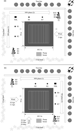
A floating perforated pipe network was used as a synthetic distributed lagoon emission source. The floating emission source was constructed of perforated, 1.3 cm schedule 40 polyvinyl chloride pipe assembled into a 45 m × 45 m grid. The grid was set up with an “I”-shaped manifold connected to a cylinder of compressed CH₄ gas. Laterals were connected at 3-m intervals along the manifold (16 laterals in total) and each lateral had 44 holes (1.6 mm diameter) drilled at 1-m intervals along the entire length. Circular foam floats were threaded onto each section of the laterals and manifold to float the entire grid on the water surface. The floating grid was secured in the center of the pond so that the laterals were in the northwest (NW)-southeast (SE) plane.

The perforated pipe network was designed to provide a uniform discharge flow from all orifices over the entire network. Pure CH₄ gas (99% CP grade CH₄; Airgas, Inc., Florence, SC) was used as a test gas, and its true emission rate was calculated from weight loss during experiments. The weight loss of the CH₄ gas cylinder was measured with a 100-kg digital platform scale (Ohaus Champ Platform scale with CW11-2EO indicator; Pine Brook, NJ). A video camera was used to record the gas flow rate, gas cylinder weight, and time. Change in mass over time and the gas purity were used to calculate the actual emission rate. The CH₄ emission rates for all experiments ranged from 0.3 to 0.4 mg m⁻² sec⁻¹, similar to the CH₄ emission rates from swine anaerobic lagoons (Sharpe and Harper, 1999).

Instrumentation

An open-path tunable diode laser (TDL) absorption spectrometer (GasFinder2.0 for CH₄; Boreal Laser, Inc., Spruce Grove, Alberta, Canada) mounted on an automatic positioning device (APD; model 20 Servo; Sagebrush Technology, Inc., Albuquerque, NM) and 10 retroreflectors (Rs) were used to measure PICs along the downwind berm (Figure 2). The TDL was located at the corner of the pond at the intersection of the two sides. Five Rs were placed in a line along each of the two sides of the pond. Three of the five Rs were positioned 1 m above ground level and the remaining two Rs were mounted at 5 and 9 m heights on a 10-m tower (Figure 2). Two 10-m towers were positioned at the end of the measurement line, which extended beyond the width of the pond (T1 and T2, Figure 1). The path lengths of the PICs, together with the heights of the Rs, are shown in Table 1. The automatic positioning device sequentially directed the infrared beam of the TDL to each R and created a two-dimensional vertical measurement planes parallel to each of the two downwind sides of the pond (Figure 2). At each R, the TDL collected about 12–15 downwind PIC data sets over a period of approximately 30 sec before being moved to next R. Once measurements were taken from each of the 10 Rs, thereby completing the cycle, the APD realigned the TDL with the first R starting the next measurement cycle. Continuous measurement cycles were completed throughout the test period. The TDL (1.2 m height) was set up for a sampling rate of about 1 Hz and had continuous calibration updates every 40 samples using an internal reference cell. In addition, the TDL was calibrated using an external calibration tube (5 cm inner diameter [i.d.] × 6.25 m length) with a standard 30 ppm CH₄ gas prior to the field tests (Ro et al., 2009). A more detailed description of the pond and instrumentation can be found in Ro et al. (2009) and Ro et al. (2013b).

Table 1. Path lengths of the PICs and heights of the retroreflectors

	Path Length (m)
Retroreflector	3 April 2013	Other Days	Height (m)
R1	32	27	1
R2	63	52	1
R3	97	79	1
R4	94	79	5
R5	94	79	9
R6	29	32	1
R7	55	64	1
R8	75	96	1
R9	72	96	5
R10	72	96	9

Figure 2. Setup of the VRPM technique for (a) 3 April 2013 and (b) 10, 11, and 18 April 2013 and 28 and 29 May 2013. Sensor locations (TDL, open-path tunable diode laser absorption spectrometer; R, retroreflectors; star, 3D sonic anemometer) and towers (T1, T2) in SW, NW, and NE planes.

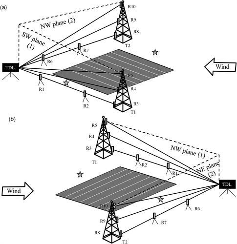
Two three-dimensional (3D) sonic anemometers (CSAT3; Campbell Scientific, Inc., Logan, UT) were used to measure wind speeds at 20 Hz. The 3D sonic anemometers provided the wind information needed for calculations of friction velocity (u*), Obukhov stability length (L), surface roughness length (z₀), and wind direction (Flesch et al., 2004). The anemometers were installed near the center of the southwest (SW) and northeast (NE) sides beside the pond and mounted on a tripod at a height of 2 m above the ground (Figures 1 and 2). The anemometers were installed facing west. The tests used the wind data obtained from one of the two anemometers simultaneously located on the upwind and the downwind berms of the pond. Additionally, two wind sensors were mounted on each of the two instrument towers at heights of 2 and 10 m, respectively. Two propeller anemometers (model 05305; R. M. Young, Traverse City, MI) were located on T1. One mechanical wind sensor (model 03001 wind sentry; Campbell Scientific) was used on T2 at a height of 2 m and a two-dimensional sonic anemometer (Windsonic; Campbell Scientific) was used on T2 at a height of 10 m.

VRPM for emission rate measurements

The coordinates of the Rs were entered into the VRPM software (Arcadis G&M, Inc., Denver, CO). The PIC data for each R were saved for reconstructing plane-integrated concentration maps for each measurement cycle and each vertical measurement plane independently. The emission rates were calculated by the software based on 15-min-averaged PICs and wind speed and direction data at 2 and 10 m heights from T1 for each measurement cycle. The VRPM data were filtered with the following criteria: (i) concordance correlation factor (CCF) >0.8 and (ii) correction factor (i.e., CCF/the Pearson correlation coefficient) >0.9. The CCF was used to represent the level of fit in reconstructing the mass-equivalent plume map based on the measured PIC data (EPA, 2006). When one optical plane was used for the VRPM calculation, only those emission rates during the cycles with wind direction (WD) between −10° and 25° from perpendicular to the plane (0°) were used as recommended by the EPA (2006).

Forward Lagrangian stochastic plume simulation

The WindTrax 2.0. software (http://www.thunderbeachscientific.com/) was also used for running the forward Lagrangian stochastic (fLS) technique to simulate downwind plume concentrations. This model releases particles from the sources and follows them forward in time as they are carried downwind. As they pass through a concentration sensor’s volume, they contribute to the concentration measured there. In the current study, the Windtrax software modeled the downwind trajectory of 5000 gas particles releasing from 30 source points (1.4 g CH₄ min⁻¹), representing a uniform CH₄ emission from the pond. The fLS technique produced CH₄ concentration plumes for each 15-min period in the planes located in each side of the pond.

Accuracy, uncertainty, and sensitive analyses

The VRPM accuracy was defined as the ratio of the emission rate determined by the VRPM technique to the actual emission rate, which was determined by dividing the decrease in the methane gas tank weight over time.

(3)

where Q is the actual emission rate (g sec⁻¹) and Q_VRPM is the calculated emission rate from the VRPM technique (g sec⁻¹).

The uncertainty in the concentration and meteorological measurements propagate in the VRPM model output. There are two types of uncertainty: type A uncertainty is determined from a series of repeated observations, whereas type B uncertainty information can be obtained from manufacturer’s specifications, understanding of instrument behavior, and uncertainties assigned to reference data taken from handbooks (Joint Committee for Guides in Metrology [JCGM], 2008). The uncertainties used in this analysis were all obtained from manufacturers’ specifications (i.e., type B uncertainties). In order to calculate the propagation of uncertainties of the VRPM model to wind speed, wind direction, path length, and the path-integrated downwind concentration, a Monte Carlo simulation method was performed with 10,000 iterations. This is a brute-force method of directly estimating a probability density function of the VRPM model outputs. It is based on performing more than 10,000 of VRPM model evaluations with randomly selected model inputs each within its uncertainty range, assuming uniform probability densities. The uncertainty ranges of input parameters were determined from typical input values encountered in actual experiments plus and minus the uncertainties specified by manufactures. The sensitivity of the VRPM model to these input parameters was estimated by evaluating 20% more and less than the input values typically encountered in the actual experiments. The percent changes of output values according to the change in each of input values were determined to assess which parameters affected the output the most or the least.

Statistical analysis was performed using the R package stats (version 3.1.0; R Core Team, 2013) for analysis of variance (ANOVA) procedure to estimate differences in accuracy data.

Results and Discussion

Accuracy of the VRPM technique

The average 10-m wind speeds during the validation studies ranged from 1.6 to 6.3 m sec⁻¹. The atmospheric stability conditions were very unstable (in 90% of data) to unstable (in 10% of data) according to Seinfeld (1986), who categorized the atmosphere as “very unstable (VU),” “unstable (U),” “neutral (N),” “stable (S),” or “very stable (VS)” based on the Monin-Obukhov length values of “−100 m < L < 0,” “−10⁵ m ≤ L ≤ −100 m,” “|L| > 10⁵ m,” “10 m ≤ L ≤ 10⁵ m,” and “0 < L < 10 m,” respectively.

The accuracies of the VRPM technique ranged from 0.13 to 1.77 in the experiments conducted in April and May 2013. The daily-average VRPM accuracies varied from 0.65 to 0.97 with an overall average accuracy of 0.77 ± 0.32 (Table 2). These accuracies were related to the vertical measurement plane 1 or 2 (i.e., NE, NW, or SW) and are comparable with that of tracers released from flat surface terrain reported by Thoma et al.(2010), 0.83 ± 0.33. In a similar flat uniform surface setting, Ro et al. (2009) also reported the VRPM errors ranging from −13% to 22% when calculating the emission rate from a single area source.

Table 2. Number of data sets and daily-average VRPM accuracy from one vertical plane (plane 1 or 2; Q_{VRPM 1 or 2}/Q) or the combination of the two vertical planes (Q_{VRPM 1+2}/Q) according to the EPA’s criteria

	One Vertical Plane		Combination of Two Vertical Planes
Date	Number of Data Sets	QVRPM 1 or 2/Q	Number of Data Sets	QVRPM 1+2/Q
3 April 2013	21	0.66 ± 0.25 (1, SW)^a	16	0.67 ± 0.29
10 April 2013	20	0.97 ± 0.45 (2, NE)	56	1.26 ± 0.54
11 April 2013	15	0.66 ± 0.28 (2, NE)	31	0.85 ± 0.36
18 April 2013	31	0.86 ± 0.29 (1, NW)	39	0.93 ± 0.29
28 May 2013	17	0.65 ± 0.18 (1, NW)	20	0.85 ± 0.30
29 May 2013	9	0.73 ± 0.21 (1, NW)	24	0.81 ± 0.35
Overall	78 (plane 1)	0.77 ± 0.32	186	0.97 ± 0.44
	35 (plane 2)

Notes: Data are mean ± standard deviation. ^aCorresponding vertical plane (plane number, orientation).

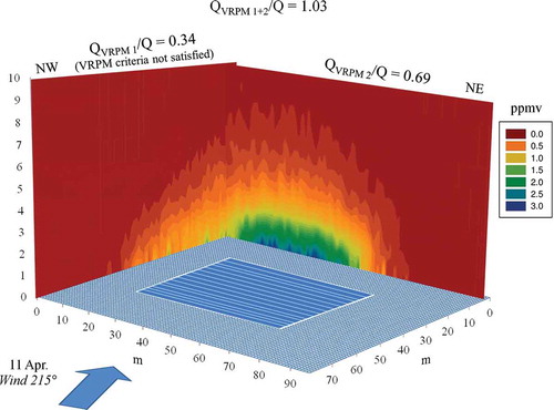
Many data sets were lost when the WD was outside of the recommended ranges, i.e., WD between −10° and 25° from perpendicular to the plane. Figure 3 shows the ideal plume captures simulated by the fLS technique in the two downwind vertical planes surrounding the lagoon (3 and 11 April 2013) where the wind was nearly perpendicular to the SW and NE, respectively. The VRPM accuracies in both cases were close to unity, which represented good measures (Ro et al., 2011). However, when wind was not perpendicular to one of the planes, the fLS model showed that the emission plume was split between the two planes (Figure 4). Consequently, low accuracies were yielded if only one vertical plane was used to calculate the emission rates (NW plane 1, Q_VRPM1/Q = 0.34 and NE plane 2, Q_{VRPM 2}/Q = 0.69 in Figure 4). If the VRPM wind direction criterion was relaxed and the two emission rates from the two optical planes were combined, the VRPM accuracy significantly improved to 1.03. In addition, the number of valid data sets also increased from 78 (plane 1 only) and 35 (plane 2 only) to 186 in the whole study. The increase in the number of data sets and the improvement of VRPM accuracies are shown in Table 2. The overall VRPM accuracy improved from 0.77 ± 0.32 with single plane to 0.97 ± 0.44 with double planes. We suggest ignoring the wind direction criteria and adding the emission rates calculated from the two downwind vertical planes surrounding the lagoon.

Figure 3. Methane emission plumes in ideal cases for VRPM technique on (a) 3 April 2013 and (b) 11 April 2013 and corresponding VRPM accuracies calculated for only plane 1 (Q_{VRPM 1}/Q) and plane 2 (Q_{VRPM 2}/Q) and the combination of both planes (Q_{VRPM 1+2}/Q). The VRPM emission data from plane 2 (Q_{VRPM 2}) did not satisfy the EPA’s filtering criteria.

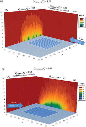
Figure 4. Methane emission plume in a nonideal case for VRPM technique in 11 April 2013 and corresponding VRPM accuracies calculated for only plane 1 (Q_{VRPM 1}/Q) and plane 2 (Q_{VRPM 2}/Q) and the combination of both planes (Q_{VRPM 1+2}/Q). The VRPM emission data from plane 1 (Q_{VRPM 1}) did not satisfy the EPA’s filtering criteria.

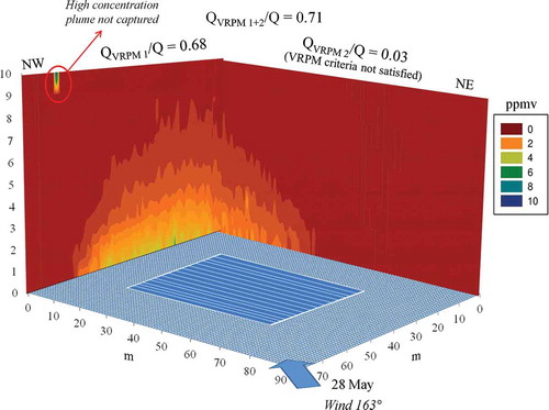
When the two 10-m towers could not capture the entire plume, the VRPM accuracy deteriorated regardless of whether the emissions from the two wind-facing planes were combined. On 28 May 2013, the entire emission was not captured by the 10-m tower. The plume picture generated by the fLS model shows a small pocket of high concentration plume at 10 m of the NW plane (Figure 5). The VRPM accuracy of this plane was unacceptably low (Q_{VRPM 1}/Q < 0.7), and the combination of both planes did not increase significantly the overall accuracy (Q_{VRPM 1+2}/Q = 0.71). The tower was not high enough to capture the whole plume of the NW plane. This coincided with McBain and Desjardins (2005), who reported that the applicability of mass-balance methods in on-farm studies is often limited by the maximum practical measurement height that can be achieved.

Figure 5. Methane emission plume in a case with the whole emission not being captured by the VRPM technique in 28 May 2013 and corresponding VRPM accuracies calculated for only plane 1 (Q_{VRPM 1}/Q) and plane 2 (Q_{VRPM 2}/Q) and the combination of both planes (Q_{VRPM 1+2}/Q). The VRPM emission data from plane 2 (Q_{VRPM 2}) did not satisfy the EPA’s filtering criteria.

Uncertainty and sensitivity of the VRPM technique

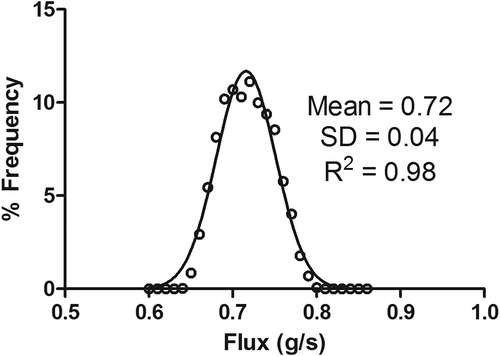
Table 3 shows the range of input parameters used for the Monte Carlo uncertainty analysis. Assuming a uniform probability distribution, the values of the parameters were randomly selected to run the VRPM model 10,000 times. Figure 6 shows that the VRPM emission rates from the Monte Carlo analysis closely resembled a normal distribution, with a mean of 0.72 g sec⁻¹ and a standard deviation of 0.04 g sec⁻¹ (i.e., coefficient of variation = 5.6%). This coefficient of variation (CV) in VRPM outputs due to the uncertainty in analytical and meteorological instruments was significantly smaller than that of VRPM accuracy ranging from 28% to 46% in Table 2 (P < 0.0001). In other words, there were factors (e.g., not capturing whole plume) other than instrumentation uncertainties that contributed to the deviation of the VRPM output emission rates from the actual emission rates.

Table 3. Range of VRPM input parameters used for the Monte Carlo analysis

Input Parameters	Typical Value	Uncertainty
Path length 1	27.0 m	±0.5 m
Path length 2	52.0 m	±0.5 m
Path length 3	79.2 m	±0.5 m
Path length 4	79.2 m	±0.5 m
Path length 5	79.2 m	±0.5 m
Wind speed at 2 m	3.1 m sec^−1	±0.1 m sec^−1
Wind speed at 10 m	3.9 m sec^−1	±0.1 m sec^−1
Wind direction at 2 m	143°	±3°
Wind direction at 10 m	143°	±3°
Concentration 1	1.95 ppm	±5%
Concentration 2	2.94 ppm	±5%
Concentration 3	1.42 ppm	±5%
Concentration 4	0.52 ppm	±5%
Concentration 5	0.21 ppm	±5%

Figure 6. VRPM emission rates from the Monte Carlo uncertainty analysis (M = 10,000).

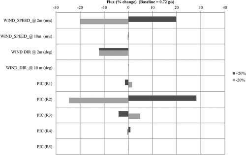
The VRPM emission rates were sensitive to the wind speed and direction at 2 m height, but not sensitive to those at 10 m height (Figure 7). This sensitivity at the lower height was probably due to the fact that the plume concentration at the higher height was too low to influence the emission rate. Among five PICs, the PIC from R2 had the highest sensitivity, probably due to its location at the center of the plume. The results of the sensitivity analysis showed that the concentration, wind speed, and wind direction near the ground were the critical parameters influencing the VRPM emission rates.

Figure 7. Sensitivity analysis of the VRPM model toward various input parameters.

Conclusion

This study evaluated the accuracy of the VRPM technique in measuring lagoon gas emission using a synthetic lagoon with a known emission rate. The VRPM yielded an average accuracy of 0.77 ± 0.32 when only one vertical plane perpendicular to the wind direction was considered. Monte Carlo uncertainty analysis showed that the VRPM emission rates varied with a CV of 5.6% due to the concentration and meteorological sensor uncertainties. This CV was significantly smaller than that of VRPM accuracy, indicating factors other than sensor uncertainties contributed to the VRPM inaccuracy such as not capturing the whole plume. The sensitivity analysis showed that the concentration near the center of plume, wind speed, and direction near the ground were the most critical parameters influencing the VRPM outputs. When both planes facing the wind were considered, ignoring the normal wind direction requirement, the accuracy of VRPM significantly improved to 0.97 ± 0.44, with substantially more valid data sets. Therefore, when using the VRPM technique for measuring lagoon gas emission, we suggest adding the emissions from the two wind-facing planes around the lagoon. These results demonstrated that the VRPM technique could be used to measure lagoon emissions with reasonable accuracy using both downwind planes facing the wind.

Acknowledgment

The authors would like to acknowledge the technical support provided by Ray Winans, Joe Millen, William Brigman, and Jerry H. Martin II of the USDA-ARS Coastal Plains Soil, Water and Plant Research Center, Florence, South Carolina. Mention of trade names or commercial products is solely for the purpose of providing specific information and does not imply recommendation or endorsement by the U.S. Department of Agriculture.

Funding

This research is part of the USDA-ARS National Programs 211 Water Availability and Watershed Management and 214 Agricultural and Industrial Byproduct Utilization. Maialen Viguria holds a grant from the Ph.D. student research program of the Department of Education, Universities and Research of the Basque Government.

Additional information

Funding

This research is part of the USDA-ARS National Programs 211 Water Availability and Watershed Management and 214 Agricultural and Industrial Byproduct Utilization. Maialen Viguria holds a grant from the Ph.D. student research program of the Department of Education, Universities and Research of the Basque Government.

Notes on contributors

Maialen Viguria

Maialen Viguria is Ph.D. in Environmental Engineering NEIKER-Tecnalia, Basque Institute for Agricultural Research and Development, in Derio, Spain.

Kyoung S. Ro

Kyoung S. Ro and Kenneth C. Stone are research engineers and Melvin H. Johnson is an agricultural engineer at the USDA-ARS Coastal Plains Soil, Water and Plant Research Center, in Florence, South Carolina, USA.

References

- Aneja, V.P., J.P. Chauhan, and J.T. Walker. 2000. Characterization of atmospheric ammonia emissions from swine waste storage and treatment lagoons. J. Geophys. Res. 105:11535–11545. doi:10.1029/2000JD900066
- Beline, F., J. Martinez, C. Marol, and G. Guiraud. 1998. Nitrogen transformations during anaerobically stored N-15-labelled pig slurry. Bioresour. Technol. 64:83–88. doi:10.1016/S0960-8524(97)84352-0
- Blanes-Vidal, V., M. Guardia, X.R. Dai, and E.S. Nadimi. 2012. Emissions of NH3, CO2 and H2S during swine wastewater management: Characterization of transient emissions after air-liquid interface disturbances. Atmos. Environ. 54:408–418. doi:10.1016/j.atmosenv.2012.02.046
- Denmead, O.T. 2008. Approaches to measuring fluxes of methane and nitrous oxide between landscapes and the atmosphere. Plant Soil 309:5–24. doi:10.1007/s11104-008-9599-z
- Denmead, O.T., J.R. Simpson, and J.R. Freney. 1977. Direct field measurement of ammonia emission after injection of anhydrous ammonia. Soil Sci. Soc. Am. J. 41:1001–1004. doi:10.2136/sssaj1977.03615995004100050039x
- Flesch, T.K., J.D. Wilson, L.A. Harper, B.P. Crenna, and R.R. Sharpe. 2004. Deducing ground-to-air emissions from observed trace gas concentrations: A field trial. J. Appl. Meteorol. 43:487–502. doi:10.1175/1520-0450(2004)043<0487:DGEFOT>2.0.CO;2
- Gao, Z., R.L. Desjardins, and T.K. Flesch. 2009. Comparison of a simplified micrometeorological mass difference technique and an inverse dispersion technique for estimating methane emissions from small area sources. Agric. Forest Meteorol. 149:891–898. doi:10.1016/j.agrformet.2008.11.005
- Grant, R.H., M.T. Boehm, and A.F. Lawrence. 2013. Comparison of a backward-Lagrangian stochastic and vertical radial plume mapping methods for estimating animal waste lagoon emissions. Agric. Forest Meteorol. 180:236–248. doi:10.1016/j.agrformet.2013.06.013
- Harper, L.A., R.R. Sharpe, and T.B. Parkin. 2000. Gaseous nitrogen emissions from anaerobic swine lagoons: Ammonia, nitrous oxide, and dinitrogen gas. J. Environ. Qual. 29(4):1356–65. doi:10.2134/jeq2000.00472425002900040045x
- Hu, E., E.L. Babcock, S.E. Bialkowsky, S.B. Jones, and M. Tuller. 2014. Methods and techniques for measuring gas emissions from agricultural and animal feeding operations. Crit. Rev. Anal. Chem. 44:200–219. doi:10.1080/10408347.2013.843055
- Intergovernmental Panel on Climate Change. 2013. Climate Change 2013: The Physical Science Basis. Contribution of Working Group I to the Fifth Assessment Report of the Intergovernmental Panel on Climate Change. https://www.ipcc.ch/report/ar5/wg1/ (accessed April 20, 2014).
- Joint Committee for Guides in Metrology. 2008. Evaluation of Measurement Data Guide to the Expression of Uncertainty in Measurement, 1st ed. Sevres, Frances: Bureau International des Poids et Mesures. http://www.bipm.org/en/publications/guides/gum.html (accessed September 8, 2014).
- Martinez, J., F. Guiziou, P. Peu, and V. Gueutier. 2003. Influence of treatment techniques for pig slurry on methane emissions during subsequent storage. Biosyst. Eng. 85:347–354. doi:10.1016/S1537-5110(03)00067-9
- McBain, M.C., and R.L. Desjardins. 2005. The evaluation of a backward Lagrangian stochastic (bLS) model to estimate greenhouse gas emissions from agricultural sources using a synthetic tracer source. Agric. Forest Meteorol. 135:61–72. doi:10.1016/S1537-5110(03)00067-9
- McGinn, S.M. 2013. Developments in micrometeorological methods for methane measurements. Animal 7(Suppl. 2):386–393. doi:10.1017/S1751731113000657
- Park, K.H., A.G. Thompson, M. Marinier, K. Clark, and C. Wagner-Riddle. 2006. Greenhouse gas emissions from stored liquid swine manure in a cold climate. Atmos. Environ. 40(4):618–27. doi:10.1016/j.atmosenv.2005.09.075
- R Core Team. 2013. R: A Language and Environment for Statistical Computing. Vienna, Austria: R Foundation for Statistical Computing. http://www.R-project.org (accessed May 31, 2014).
- Ro, K.S., M.H. Johnson, P.G. Hunt, and T.K. Flesch. 2011. Measuring trace gas emission from multi-distributed sources using vertical radial plume mapping (VRPM) and backward Lagrangian stochastic (bLS) techniques. Atmosphere 2:553–566. doi:10.3390/atmos2030553
- Ro, K.S., M.H. Johnson, K.C. Stone, P.G. Hunt, T. Flesch, and R.W. Todd. 2013. Measuring gas emissions from animal waste lagoons with an inverse-dispersion technique. Atmos. Environ. 66:101–106. doi:10.1016/j.atmosenv.2012.02.059
- Ro, K.S., M.H. Johnson, R.M. Varma, R.A. Hashmonay, and P. Hunt. 2009. Measurement of greenhouse gas emissions from agricultural sites using open-path optical remote sensing method. J. Environ. Sci. Health A 44:1011–1018. doi:10.1080/10934520902996963
- Ro, K.S., K.C. Stone, M.H. Johnson, P.G. Hunt, T.K. Flesch, and R.W. Todd. 2014. Optimal sensor locations for the backward Lagrangian stochastic technique in measuring lagoon gas emission. J. Environ. Qual. 43:1111–1118
- Sanz-Cobena, A., T.H. Misselbrook, A. Arce, J.I. Mingot, J.A. Diez, and A. Vallejo. 2008. An inhibitor of urease activity effectively reduces ammonia emissions from soil treated with urea under mediterranean conditions. Agric. Ecosyst. Environ. 126:243–249. doi:10.1016/j.agee.2008.02.001
- Seinfeld, J.H. 1986. ES books: Atmospheric chemistry and physics of air pollution. Environ. Sci. Technol. 20:863–863. doi:10.1021/es00151a602
- Sharpe, R.R., and L.A. Harper. 1999. Methane emissions from an anaerobic swine lagoon. Atmos. Environ. 33:3627–3633. doi:10.1016/S1352-2310(99)00104-1
- Sharpe, R.R., L.A. Harper, and F.M. Byers. 2002. Methane emissions from swine lagoons in southeastern US. Agric. Ecosyst. Environ. 90:17–24. doi:10.1016/S0167-8809(01)00305-X
- Sommer, S.G., S.M. McGinn, and T.K. Flesch. 2005. Simple use of the backwards Lagrangian stochastic dispersion technique for measuring ammonia emission from small field-plots. Eur. J. Agron. 23:1–7. doi:10.1016/j.eja.2004.09.001
- Thoma, E.D., R.B. Green, G.R. Hater, C.D. Goldsmith, N.D. Swan, M.J. Chase, and R.A. Hashmonay. 2010. Development of EPA OTM 10 for landfill applications. J. Environ. Eng. 136:769–776. doi:10.1061/(ASCE)EE.1943-7870.0000157
- U.S. Environmental Protection Agency. 2006. Other Test Method 10 (OTM 10)—Optical Remote Sensing for Emission Characterization from Non-point Sources. Washington, DC: U.S. Environmental Protection Agency.
- van der Peet-Schwering, C.M.C., A.J.A. Aarnink, H.B. Rom, and J.Y. Dourmad. 1999. Ammonia emissions from pig houses in the Netherlands, Denmark and France. Livest. Prod. Sci. 58:265–269. doi:10.1016/S0301-6226(99)00017-2
- Wilson, J.D., V.R. Catchpoole, O.T. Denmead, and G.W. Thurtell. 1983. Verification of a simple micrometeorological method for estimating the rate of gaseous mass-transfer from the ground to the atmosphere. Agric. Meteorol. 29:183–189. doi:10.1016/0002-1571(83)90065-1