Air Quality and Climate Connections

Abstract

Multiple linkages connect air quality and climate change. Many air pollutant sources also emit carbon dioxide (CO₂), the dominant anthropogenic greenhouse gas (GHG). The two main contributors to non-attainment of U.S. ambient air quality standards, ozone (O₃) and particulate matter (PM), interact with radiation, forcing climate change. PM warms by absorbing sunlight (e.g., black carbon) or cools by scattering sunlight (e.g., sulfates) and interacts with clouds; these radiative and microphysical interactions can induce changes in precipitation and regional circulation patterns. Climate change is expected to degrade air quality in many polluted regions by changing air pollution meteorology (ventilation and dilution), precipitation and other removal processes, and by triggering some amplifying responses in atmospheric chemistry and in anthropogenic and natural sources. Together, these processes shape distributions and extreme episodes of O₃ and PM. Global modeling indicates that as air pollution programs reduce SO₂ to meet health and other air quality goals, near-term warming accelerates due to “unmasking” of warming induced by rising CO₂. Air pollutant controls on CH₄, a potent GHG and precursor to global O₃ levels, and on sources with high black carbon (BC) to organic carbon (OC) ratios could offset near-term warming induced by SO₂ emission reductions, while reducing global background O₃ and regionally high levels of PM. Lowering peak warming requires decreasing atmospheric CO₂, which for some source categories would also reduce co-emitted air pollutants or their precursors. Model projections for alternative climate and air quality scenarios indicate a wide range for U.S. surface O₃ and fine PM, although regional projections may be confounded by interannual to decadal natural climate variability. Continued implementation of U.S. NO_x emission controls guards against rising pollution levels triggered either by climate change or by global emission growth. Improved accuracy and trends in emission inventories are critical for accountability analyses of historical and projected air pollution and climate mitigation policies.

Implications: The expansion of U.S. air pollution policy to protect climate provides an opportunity for joint mitigation, with CH₄ a prime target. BC reductions in developing nations would lower the global health burden, and for BC-rich sources (e.g., diesel) may lessen warming. Controls on these emissions could offset near-term warming induced by health-motivated reductions of sulfate (cooling). Wildfires, dust, and other natural PM and O₃ sources may increase with climate warming, posing challenges to implementing and attaining air quality standards. Accountability analyses for recent and projected air pollution and climate control strategies should underpin estimated benefits and trade-offs of future policies.

View correction statement:

Corrigendum

Introduction

Climate and air quality are inextricably connected. Many sources of “conventional” air pollutants are also sources of CO₂, other GHGs (see Table 1 for list of acronyms), and/or particles that affect climate (see Key Terms). These air pollutants interact with solar and terrestrial radiation and perturb the planetary energy balance, leading to changes in climate (Intergovernmental Panel on Climate Change [IPCC], 2013a). Climate change influences air pollution by altering the frequency, severity, and duration of heat waves, air stagnation events, precipitation, and other meteorology conducive to pollutant accumulation (e.g., Jacob and Winner, 2009; Weaver et al., 2009; Ordóñez et al., 2005; Tressol et al., 2008; Vieno et al., 2010). We focus on PM and O₃ and their major components and precursors; these two air pollutants are responsible for the most widespread violations of the U.S. National Ambient Air Quality Standards (NAAQS) (Environmental Protection Agency [EPA], 2013), and contribute to climate change (Table 2).

Arlene M. Fiore

Table 1. Acronyms.

AAOD	aerosol absorption optical depth
ACCMIP	Atmospheric Chemistry and Climate Model Intercomparison Project
AeroCom	Aerosol Comparisons between Observations and Models
AOD	aerosol optical depth
AR5	Fifth Assessment Report of the IPCC
BC	black carbon
BrC	brown carbon
CASTNet	Clean Air Status and Trends Network
CCM	chemistry–climate model
CCN	cloud condensation nuclei
CCSP	Climate Change Science Program
CLE	current legislation
CMIP	Coupled Model Intercomparison Project
CTM	chemistry-transport model
DU	Dobson unit
ENSO	El Niño Southern Oscillation
EPA	Environmental Protection Agency
ERF	effective radiative forcing
ERFaci	ERF due to aerosol–cloud interaction
ERFari	ERF due to aerosol–radiation interaction
GCM	general circulation model
GHG	greenhouse gas
GMST	global mean surface temperature
GWP	global warming potential
HCFC	hydrochlorofluorocarbons
HFC	hydrofluorocarbons
IAM	integrated assessment model
IN	ice nuclei
IPCC	Intergovernmental Panel on Climate Change
ITCZ	InterTropical Convergence Zone
MDA8	daily maximum 8-hourly average ozone concentration
MFR	maximum feasible reduction
NAAQS	National Ambient Air Quality Standards
NARCCAP	North American Regional Climate Change Assessment Program
NMVOC	nonmethane volatile organic compounds
NRC	National Research Council of the U.S. National Academy of Sciences
NTCF	near-term climate forcer
OC	organic carbon
PAN	peroxyacetylnitrate
PM	particulate matter
RCP	representative concentration pathway
RCTM	regional chemistry-transport model
RF	radiative forcing
RFari	RF due to aerosol-radiation interaction
RCM	regional climate model
RTM	radiative transfer model
SLCF	short-lived climate forcer
SLCP	short-lived climate pollutant
SOA	secondary organic aerosol
SRES	Special Report on Emission Scenarios
TF HTAP	Task Force on Hemispheric Transport of Air Pollution
WG1	Working Group 1 of the IPCC

Table 2. Near-term climate forcing air pollutants (and precursors) with CO₂ shown for comparison; although emissions for SLCPs are much smaller than CO₂, they have much larger GWPs^a over 100 years.

Pollutant	Lifetime	Major sources	Anthropogenic emissions^b	GWP^c100
Methane (CH4)	~10 years	Agriculture (livestock, rice production), oil and gas systems, coal mining, waste management	350 Tg CH4	29
Tropospheric ozone (O3)	Days (near-surface, summer) to months (free troposphere, winter)	Multiple sources of precursors (see Figure 2)
		CH4 (above)
		Carbon monoxide (CO)	1040 (Tg yr ^−1)	1.9
		Nitrogen oxides (NOx)	39 (Tg N yr^−1)	–11^d
		Nonmethane volatile organic compounds (NMVOC)	210 (Tg yr^−1)	4.5^h
Black carbon (BC)	Days to weeks	Open biomass burning, residential cooking and heating with biomass and coal, industrial coal, diesel engines	8.2 (Tg yr^−1)	660
				900^e
Organic carbon (OC)	Days to weeks	Same as BC for directly emitted OC; secondary organics from some biogenic and anthropogenic precursor gases	36 (Tg yr^−1)	–66^f
Sulfur oxides (SOx)	Days	Energy-related fossil fuel combustion, industrial processes such as metal smelting, marine shipping	54 (Tg S yr^−1)	–38
CO2	100 to ≫1000 years	Fossil fuel combustion, cement production, land-use change^g	10 (Pg C yr^−1)	1

Notes: ^aGlobal Warming Potential (GWP; see Key Terms) is an imperfect measure used to compare the relative warming produced by different pollutants relative to CO₂ over a period of time (here, 100 years). A ton of CH₄ emissions is 28.5 times more potent than a ton of CO₂ over 100 years. The short lifetimes of the non-CH₄ O₃ precursors and PM components result in higher values for nearer time periods (e.g., GWP₁₀). GWPs for precursors reflect forcing from secondary products including sulfate and nitrate aerosols, O₃, and indirect effects on reactive GHGs (e.g., CH₄). See also Figure 1.

^bPresent-day estimates (~2010) from IPCC AR5 WGI (Ciais et al., 2013; Myhre et al., 2013a; IPCC, 2013b).

^cFrom Table 8.SM.17 of Myhre et al. (2013a).

^dThe net negative represents competition between NO_x-induced increases in O₃ (warming) versus decreases in CH₄ (cooling), which cause the GWP for nearer time periods (GWP₁₀ or GWP₂₀) to be positive.

^eFrom Bond et al. (2013). Range of 120 to 1800 including all forcing mechanisms.

^fEven more uncertain than estimates for the other highly uncertain short-lived species because this estimate assumes OC is scattering (cooling) but there is some evidence for a stronger contribution from absorbing (warming) organic particles (see main text).

^gIncludes conversion of forests to agriculture and other human-induced transitions to land cover; biofuel and open burning are included to the extent that these activities are a net source of atmospheric CO₂.

^hFrom Table 8.A.5 of Myhre et al. (2013).

A measure of the perturbation to the climate system due to changes in various atmospheric constituents between the preindustrial and present day atmosphere is radiative forcing (RF; Figure 1). Positive RF induces a warming, whereas negative RF induces a cooling of the earth’s surface and troposphere. The increase in the atmospheric burdens of GHGs, including CO₂, and that of tropospheric O₃ and its precursor methane (CH₄) over the past few centuries have exerted a warming influence. In contrast, the net effect of PM (termed “aerosols” in Figure 1, as conventional in climate science) is to cool the planet, although the magnitude is much more uncertain than for the GHGs. This net cooling effect of PM reflects offsetting influences from warming BC and “brown” organic carbon (BrC) particles versus cooling sulfate, nitrate, and other OC particles. All individual PM components can interact with clouds, disrupting natural precipitation and circulation patterns (e.g., Boucher et al., 2013; Bond et al., 2013).

Figure 1. Globally averaged radiative forcing (RF; see Key Terms) of climate from preindustrial (1750) to present (2011) of air pollutants and their precursor emissions, as compared to carbon dioxide (CO₂) emissions. PM components (also referred to as aerosols) include sulfate, nitrate, black carbon (BC), organic carbon (OC) and dust. The RF from aerosol–radiation interactions is shown for aerosol components except for “aerosol–cloud,” which is the effective radiative forcing (ERF; see Key Terms) from aerosol–cloud interactions. Values are the IPCC (2013a) best estimates assessed by Myhre et al. (2013a; their Table 8.SM.6; colored bars), with uncertainty ranges (their Table 8.SM.7; black vertical bars). Through atmospheric chemistry, many emitted species (methane [CH₄], carbon monoxide [CO], nonmethane volatile organic compounds [NMVOC], nitrogen oxides [NO_x], ammonia [NH₃], and sulfur dioxide [SO₂]) influence multiple atmospheric constituents (“Radiative Forcing Components”). Also shown are BC and OC RFs from biofuel and fossil fuel combustion (BF + FF), from biomass burning (BB) and from BC deposited on snow (Snow Alb.). Rapid adjustments to all aerosol-radiation interactions reduce the ERF by –0.1 W m² (Table 8.6; Myhre et al., 2013a). The total global average anthropogenic RF for all components (including additional GHGs such as halocarbons and nitrous oxide, and land-use change) is +2.3 W m⁻² (90% confidence range of +1.1 to +3.3 W m⁻²; Myhre et al., 2013a).

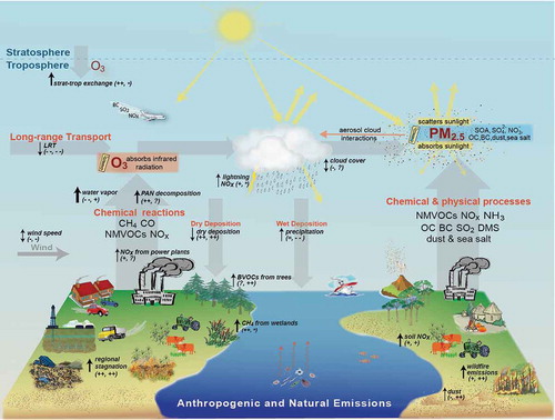
Interactions between air quality and climate occur on multiple space and time scales, through various mechanisms (Figure 2). Tropospheric O₃ forms from photochemical reactions involving nitrogen oxides (NO_x), nonmethane volatile organic compounds (NMVOCs), CH₄, or carbon monoxide (CO). Fine PM with diameter smaller than 2.5 µm (PM_2.5) is both directly emitted from surface sources (primary PM) and formed in the atmosphere through gas- and aqueous-phase chemical reactions among precursor species (secondary PM). Direct emissions are the main sources of sea salt, mineral dust, and BC and OC from combustion. Secondary components include sulfate (via oxidation of precursor gases SO₂ and dimethyl sulfide [DMS]), ammonium nitrate (via reactions of NO_x and NH₃ gases), and secondary organic aerosols (SOA; via oxidation of some NMVOCs). The abundance of all secondary aerosols also depends on anthropogenic influences that affect aerosol formation from emitted precursors (Unger et al., 2006; Carlton et al., 2010; Shindell et al., 2009; Leibensperger et al., 2011).

Figure 2. Air quality and climate connections, following Figure 2 of Isaksen et al. (2009), Table 1 of Jacob and Winner (2009), and Table 1 of Fiore et al. (2012). Anthropogenic and natural emitted species include CH₄, CO, NMVOC, NO_x, SO_2, NH₃, OC, BC, dimethyl sulfide (DMS; from oceanic biota), mineral dust, and sea salt. Orange text describes atmospheric processing (formation, removal, and transport) of air pollutants. Black text with black arrows indicates the sensitivity of these processes to climate warming; thinner arrows denote lower confidence or regional variability in the sign of the change (increase is up; decrease is down; double-headed arrow implies no clarity on the sign of change) in response to a warming climate. Dual black symbols in the parentheses indicate how (O₃, PM) respond to the change indicated for each process (for double-headed arrows, the (O₃, PM) response denoted is for an increase in the process): ++ consistently positive, + generally positive, = weak or variable; - generally negative, – consistently negative, ? uncertainty in the sign of the response, and * the response depends on changing oxidant levels. Not shown are primary biological aerosol particles (PBAP; e.g., pollen, fungi, bacteria, algae, and viruses), which may affect climate (Després et al., 2012).

The production, distribution, and combustion of fossil fuels (e.g., in power plants, residential heating and cooling, on-road and off-road vehicles, ships, and aircraft) are major sources of PM and O₃ precursors, and CO₂ to the atmosphere. Anthropogenic CH₄ is emitted from agricultural activities (e.g., raising livestock), and from landfills and wastewater treatment facilities. The inadvertent release during production of natural gas, particularly through hydraulic fracturing operations, is receiving attention (e.g., Brandt et al., 2014). Many air pollutants and GHGs have natural sources: Wildfires produce all of the species shown in Figure 2; the terrestrial biosphere emits NMVOCs and NO_x; the oceanic biosphere is a source of sulfur dioxide (SO₂, via oxidation of DMS) and possibly OC (e.g., Quinn and Bates, 2011). Sea salt aerosol is considered natural, while the source of mineral dust can be influenced by human activities (Ginoux et al., 2012). Lightning is a source of NO_x, and volcanoes release SO₂. The largest single source of CH₄ is from wetlands. Many of these species are removed from the atmosphere by chemical reactions, photolysis, or deposition to the surface. PM is removed by both wet and dry deposition, with higher rates of wet deposition for the soluble species and mixtures that dominate the fine fraction.

Key Terms

Classes of climate forcing atmospheric constituents

Greenhouse gases (GHGs) are gaseous atmospheric constituents that absorb and emit specific wavelengths of terrestrial radiation such that radiation that would otherwise escape to space is trapped, leading to surface and tropospheric warming (IPCC, 2013d). Major greenhouse gases include natural and anthropogenic constituents such as water vapor, CO₂, nitrous oxide, CH₄, and O₃, along with gases such as sulfur hexafluoride (SF6), chlorofluorocarbons (CFCs), hydrofluorocarbons (HFCs), and perfluorocarbons (PFCs) that are entirely human-made. Aside from water vapor, O₃, and some HFCs, these gases are sufficiently long-lived as to be fairly well mixed in the troposphere such that a few measurements at remote locations on the earth’s surface can reliably be used to estimate the tropospheric burden; this subset of GHGs is often referred to as well-mixed greenhouse gases (WMGHGs; see Box 8.2 of Myhre et al., 2013a).

Near-term climate forcers (NTCFs) and short-lived climate forcers (SLCFs) are defined as radiatively active atmospheric constituents, and their precursors, whose impact on climate occurs primarily in the first one to three decades (near term) after their emission, such as O₃, aerosols, and CH₄ (Myhre et al., 2013a). While SLCF has been widely used in the published literature, IPCC (2013a) adopts the NTCF terminology since it clearly includes CH₄ (also a WMGHG), avoiding the ambiguity as to whether CH₄ is “short-lived” (it is relative to CO₂, but not compared to most air pollutants such as BC or tropospheric O₃ for example).

Short-lived climate pollutants (SLCPs) are the subset of NTCFs that have a warming influence on the climate system. The Clean Air and Climate Coalition (CCAC) names CH₄, tropospheric O₃, HFCs, and BC as the major SLCPs (CCAC, 2014).

Metrics for comparing climate impacts

Radiative forcing (RF) is defined as the perturbation in the net radiative flux (W m⁻²) at the tropopause or top of the atmosphere, typically after allowing stratospheric temperatures to adjust but holding all surface and tropospheric conditions fixed, that occurs due to a change in the atmospheric abundance or distribution of a radiatively active atmospheric constituent (IPCC, 2013d). It is common practice to report RF as that induced by differences between present-day and preindustrial atmospheric burdens of a particular atmospheric constituent, in order to quantify the anthropogenic contribution. IPCC (2013a) uses 1750 as the beginning of the industrial era. The RF modifies the energy balance of the earth system, inducing changes in the earth’s surface temperature in order to reestablish equilibrium (a balanced energy budget).

Effective radiative forcing (ERF) is the change in the net top-of-the-atmosphere downward radiative flux induced by a change in GHGs or aerosols, after allowing for physical quantities such as atmospheric temperatures, water vapor, and clouds, but not the ocean or sea ice, to adjust (IPCC, 2013d). For PM, ERF thus includes both aerosol–radiation interactions and aerosol–cloud interactions. Including these rapid adjustments in the ERF is thought to provide a better estimate of the eventual temperature response to atmospheric perturbations to these constituents than RF (Boucher et al., 2013; Myhre et al., 2013a). For many non-aerosol constituents, rapid adjustments are not well characterized (e.g., tropospheric O₃), so the RF metric is used.

Global warming potential (GWP) is a metric commonly used to compare climate impacts of an atmospheric constituent relative to CO₂. Specifically, GWP measures the integrated RF following a pulse unit mass emission of an atmospheric constituent relative to that of a unit mass of CO₂ over a selected time period, combining the effects of atmospheric lifetimes and potency (i.e., efficacy of trapping terrestrial radiation) relative to CO₂ (IPCC, 2013d). The most common choice for time period is 100 years (GWP₁₀₀ shown in Table 2), but some favor 20 years for SLCPs. The choice of time scale implicitly includes value judgments (Myhre et al., 2013a). The strengths and limitations of this metric are discussed in Myhre et al. (2013a); a notable weakness is that GWP cannot convey information regarding regional climate responses unless they scale directly with global RF.

Climate penalty is either the increase in surface O₃ resulting from regional climate warming in the absence of precursor emission changes or the additional precursor emission reductions needed to achieve a targeted level of air quality in a warmer climate (Wu et al., 2008a). Bloomer et al. (2009) defined the “climate penalty factor” as the slope of the local-to-regional observed O₃-temperature relationship. This observed “climate penalty factor” may not be a good indicator of the “climate penalty” if the observed relationship is not stationary (i.e., reflects a common dependence of temperature and O₃ on another driver).

Return level describes the probability of exceeding a specified value of some quantity of interest within a specified time window using statistical methods from extreme value theory. These methods are commonly used to quantify hydrological extremes, for example, the level of the “50-year” flood. In an analogous manner, Figure 11 shows return levels for the 1-year summertime O₃ event, corresponding to the probability of observing an O₃ event of that level or higher on one out of 92 summer days.

The climate variables depicted in Figure 2 represent local thermodynamic responses as well as broader changes in atmospheric circulation, which may undergo climatological shifts in response to changes in the energy budget induced by perturbing the abundances of GHGs and PM. These changes in climate affect the sources and sinks of air pollutants (Figure 2). They also alter the chemical and transport processes modulating the formation and accumulation of pollution from the near-surface atmosphere where they are hazardous to human health, vegetation, and the built environment. For example, numerous studies highlight the potential for more frequent drought in the southwestern U.S. as the climate warms; the resulting impacts on wildfires and dust could worsen PM pollution (Seager et al., 2007; Cook et al., 2009; Spracklen et al., 2009; Flannigan et al., 2009). The potential for climate warming to exacerbate O₃ pollution in populated (polluted) regions (Jacob and Winner, 2009; Weaver et al., 2009; Fiore et al., 2012; Kirtman et al., 2013) has led to widespread use of the term climate penalty (Wu et al., 2008a; see Key Terms) to convey the adverse impact of climate change on air pollution. These strong connections between air pollution and climate underlie calls for a more coordinated approach to addressing climate change and air quality goals (e.g., Ravishankara et al., 2012).

Air quality management faces multiple challenges. Health-based evidence supports tighter air quality standards. A lower O₃ NAAQS level may be set in 2015, and the PM_2.5 annual mean NAAQS was lowered in 2012. Lower NAAQS levels raise the relative importance of background levels, which do not respond directly to regulated U.S. emission sources, but include components such as global CH₄ or transported foreign pollution that might be addressed through international negotiations (e.g., Task Force on Hemispheric Transport of Air Pollution [TF HTAP], 2010a, 2010b, 2010c). CH₄ is not presently regulated as an O₃ precursor in the U.S., as its lifetime of about a decade precludes it from contributing to local or regional O₃ pollution episodes, though it does increase background O₃ levels in surface air (Fiore et al., 2002). The recent addition of climate goals to U.S. air pollution policy raises the profile of CH₄ emission reductions for attaining air quality and climate goals simultaneously (EPA, 2009). This expansion of scope to include climate goals further implies a need to quantify climate warming induced by health-motivated reductions of cooling PM_2.5 components such as sulfate (Raes and Seinfeld, 2009) so that actions can be taken to offset this climate disbenefit. Finally, the vehicles and electricity-generating units initially targeted for CO₂ reductions have already been regulated for decades under the Clean Air Act, to improve health and reduce acid rain and visibility impairment, though those controls did not slow CO₂ emission growth (Bachmann, 2007; Watson, 2002).

In the following, we (1) describe the historical and future emissions frequently used to address both the impacts of air pollutants and their precursors on climate and the influence of climate change—and variability—on U.S. air pollution; (2) review major interactions between air quality and climate, including impacts on extreme O₃ and PM pollution events in the context of changing air pollutant emissions; (3) highlight emerging challenges to U.S. air quality management; and (4) recommend research directions aimed at supporting a more holistic approach to U.S. air pollution management and at advancing our understanding of air quality–climate connections. Throughout this critical review, we summarize findings from IPCC (2013a) and extend or revise those findings in light of newer work where possible.

Emissions of Air Pollutant NTCFs

Quantifying climate impacts from a particular species, region, or sector requires accurate global emissions. High-quality inventories are needed to underpin international agreements aimed at limiting long-range transport of air pollution (e.g., TF HTAP, 2010a) or to attain global air quality or climate goals. In some cases, emissions are directly measured (e.g., continuous emission monitors on U.S. power plant smokestacks) or modeled (e.g., from mobile and biogenic sources). At the global scale, bottom-up emissions from human activities are typically calculated as the product of activity data (e.g., energy consumption, agricultural activities, industrial production) and an emission factor for a particular chemical species per activity, and are allocated onto a geographical grid (Lamarque et al., 2010, and references therein). Several gridded regional and global emission inventories exist for air pollutants (see http://www.geiacenter.org).

Emission inventory quality varies widely because of diversity in methodology, input data, and assumptions (Granier et al., 2011). The U.S. and Europe have implemented strong air pollution control programs, spurring efforts to quantify emissions from specific sources and track their changes over time, leading to multiple estimates that are in better agreement and show consistent declines in key pollutants since the 1980s (see Figure S1; Supplemental Text S1; Granier et al., 2011). Emission inventory development and validation is supported in these regions by continuous emissions monitors, ambient monitoring networks, and air quality modeling. In sharp contrast, large uncertainties exist in emission inventories for developing countries because of a lack of emissions monitoring, lack of validation against in situ measurements, and incomplete and conflicting activity data (e.g., Bond et al., 2013; Sadavarte and Venkataraman, 2014), resulting in low-quality emission inventories (see Figure 5 of Granier et al., 2011; Amann et al., 2013; Bond et al., 2013; Smith et al., 2011; TF HTAP, 2010a).

Global air pollutant emissions have increased since 1850 and have undergone spatial and sectoral redistribution (Lamarque et al., 2010; Smith et al., 2011). Modeled preindustrial O₃ and PM distributions based on historical emission inventories generally simulate levels higher than the limited and uncertain observations (e.g., Bauer et al., 2013; Lee et al., 2013; Myhre et al., 2013a, Stevenson et al., 2013), indicating uncertainty in model-based preindustrial to present-day RF (or the effective RF) estimates discussed in the next section. New measurements from ice cores in Greenland offer the possibility of improved constraints on the temporal evolution of near-term climate forcer (NTCF) emissions since the preindustrial (Geng et al., 2015).

Due to targeted air pollution controls, anthropogenic air pollutant emissions decoupled from CO₂ in the U.S. (Bachmann, 2007; www.epa.gov/airtrends/aqtrends.html) and other developed nations (Amann et al., 2013) after peaking in the 1970s. Decreases in U.S. emissions of SO₂ and NO_x, driven by Clean Air Act requirements through federal rules and state plans since the 1970s and 1990s, respectively, are confirmed by in situ and satellite observations (de Gouw et al., 2014; Reuter et al., 2014, Russell et al., 2012; Duncan et al., 2013; Lamsal et al., 2015; Tong et al., 2015) and incorporated into more recent emission inventories (Xing et al., 2013; Klimont et al., 2013). In China, emission controls and improved energy efficiency led to SO₂ and CO emission decreases, while NO_x and VOC emissions continued to grow during 2005–2010 (Zhao Y. et al., 2013; Kurokawa et al., 2013), indicating that the latter remain tightly coupled to CO₂ and therefore to energy consumption. In contrast, air pollutant emissions from India increased rapidly after 2000, driven by growth in energy demand and absence of regulation (Kurokawa et al., 2013; Sadavarte and Venkataraman, 2014). Emissions from developing nations are more uncertain, but rapid advances in space-based estimation of emissions are anticipated when tropospheric composition is observed continuously from geostationary platforms (e.g., Hoff and Christopher, 2009; Streets et al., 2013, 2014; Chance et al., 2013). While the northern mid-latitudes will likely be well covered, maintaining global coverage as achieved with current polar-orbiting satellites or through additional geostationary platforms will be crucial for observing emission changes in the tropics and southern hemisphere.

Future air pollutant emissions scenarios have been developed systematically for use in climate modeling (see Supplemental Text S1). Air pollutant emission projections based on the IPCC Special Report on Emission Scenarios (SRES) (Nakicenovic et al., 2000) were not suitable for air quality projections, as they did not consider the emerging emissions controls in developing countries after 1990 (Amann et al., 2013), projecting continued growth in emissions (e.g., global NO_x emissions in 2100 relative to 2000 change by –12 to +175%) and model-simulated O₃ concentrations (e.g., Prather et al., 2003). To address this flaw, near-term pollutant emission scenarios were developed (Dentener et al., 2005; Cofala et al., 2007) that implement either current air quality legislation (CLE) or all technologically feasible control strategies globally regardless of cost (maximum feasible reduction, MFR) to 2030 (Dentener et al., 2005, 2006; Stevenson et al., 2006; Kloster et al., 2008). The new Representative Concentration Pathways (RCPs) (Moss et al., 2010; van Vuuren et al., 2011a) climate forcing scenarios include both air pollutants and GHGs (including stratospheric ozone depleting substances). The fundamental difference between the SRES and RCP scenarios is that the SRES versions are tied to specified socioeconomic changes while the RCPs are not, and thus multiple socioeconomic and environmental pathways can yield the same RCP RFs (Nakicenovic et al., 2014; O’Neill et al., 2014).

The four RCP scenarios span a range of RF in 2100 relative to preindustrial atmospheric composition, from 2.6 W m⁻² (assuming implementation of stringent climate policies) to 8.5 W m⁻² (no climate policy), with each RCP produced by a different integrated assessment model (IAM; Masui et al., 2011; Riahi et al., 2011; Thomson et al., 2011; van Vuuren et al. 2011b). For continuity with historical emissions (Lamarque et al., 2010; see Supplemental Text S1), the IAM emissions, projected over the 2005–2100 time period, were harmonized (set equal) to the emissions in year 2000 in the historical data set (van Vuuren et al., 2011a) to provide a temporally smoothed trajectory for global GHG abundances and gridded anthropogenic and biomass burning emissions of air pollutants and their precursors from 1850 to 2100 (Lamarque et al., 2010; Meinshausen et al., 2011; van Vuuren et al., 2011a). The models branch at 2006 into the four RCP pathways. This data set formed the basis of chemistry–climate model (CCM) simulations for the Atmospheric Chemistry and Climate Modeling Intercomparison Project (ACCMIP) (Lamarque et al., 2013) and the Coupled Model Intercomparison Project (CMIP5) (Taylor et al., 2012) studies assessed in the Fifth Assessment Report of the IPCC (IPCC AR5) (e.g., Bindoff et al., 2013; Collins M. et al., 2013; Flato et al., 2013; Kirtman et al., 2013; Myhre et al., 2013a).

Over the 21st century, all RCPs project a declining trend for O₃ and PM precursor emissions except NH₃, which rises with population and food demand in all scenarios, and CH₄ in the RCP8.5 scenario, where a high fossil-intensive energy sector combines with increasing population and associated high food demand (Riahi et al., 2011) (Figure S2). The trends in sectoral emissions differ by world regions (e.g., U.S. vs. East Asia in Figure S2). Despite growth in fossil-intensive emissions from the energy and industry sectors (particularly high in East Asia) in RCP8.5, air pollutants emissions decrease (earlier in the U.S., later in East Asia). A key feature of the RCP2.6 scenario is that it assumes bioenergy and carbon capture and storage technologies to achieve negative CO₂ emissions by the end of the 21^st century.

Two assumptions common across the RCPs drive the decline in air pollution emissions: (a) air pollution controls become stringent with time as income levels rise, and (b) climate policies aimed at controlling GHG emissions decrease air pollutant emissions from common sources (van Vuuren et al., 2011a). These assumptions lead to a small spread across the RCP global short-lived pollutant emissions. For example, the RCP aerosol and O₃ precursor emissions are factors of 1.2 to 3 smaller than SRES by 2030 (Kirtman et al., 2013). Similarly, the spread across RCP air pollutant emissions by 2030 is much smaller than the range between the CLE and MFR scenarios: ±12% versus ±31% for NO_x; ±17% versus ±60% for SO₂; ±5% versus ±11% for CO (Kirtman et al., 2013). Most of this narrow range of projected pollutant emissions in the mid to long term across the RCPs is driven by uncertainties in projecting emissions from developing nations and is not fully representative of other possible scenarios with little or no pollution controls (e.g., SRES) (Chuwah et al., 2013; Amann et al., 2013; Kirtman et al., 2013; Rogelj et al., 2014a). The small range for air pollutant emissions across the RCPs, aside from CH₄, limits their utility in gauging the range of possible future changes in air quality and in climate responses to NTCFs.

Influence of Air Pollutants on Climate

We review here recent estimates of RF and effective radiative forcing (ERF) (see Key Terms) from various air pollution-related gases and particles (Table 2), as well as estimates of changes in global and regional climate resulting from perturbations to their abundances in the atmosphere. Methods used to estimate impacts on the climate system are summarized in Table S1. A quantitative understanding of the climate effects of air pollutants is critical in the mitigation of future climate change for two principal reasons.

First, the net cooling impact of anthropogenic PM on 20th-century climate change (Figure 1) obfuscates, or “masks,” the effect of CO₂. The lack of a precise quantification of this cooling influence lessens confidence in future climate projections. If anthropogenic PM were a significant contributor to 20th-century climate, then it must have coincided with a large warming from increasing levels of CO₂ and other GHGs to produce the observed increase in global mean surface temperature (GMST; linear trend of +0.85°C from 1880 to 2012; see Supplemental Text S2; Table S2). The converse is also true: If anthropogenic PM has a small impact on climate, then the influence of the increase in CO₂ on the climate system (“climate sensitivity”; typically defined as the equilibrium GMST change from a doubling of atmospheric CO₂) is not required to be as strong to reproduce observed changes. Models with a strong response to anthropogenic PM tend to simulate a larger climate sensitivity, implying that models with strong aerosol forcing will project more warming from GHGs as the PM burden decreases (Kiehl, 2007; Knutti, 2008).

Second, an improved understanding of air pollutant impacts on climate is necessary to assess the unintended climate impacts of recent and future air quality regulations (Leibensperger et al., 2012a; Makkonen et al., 2012; Levy et al., 2013; Rotstayn et al., 2013) and the potential to mitigate near-term warming by selective emission reductions of short-lived climate pollutants (SLCPs) (e.g., Ramanathan and Xu, 2010; Schmale et al., 2014), the warming subset of NTCFs (see Table 2 and Key Terms). Uncertainties in the location and strength of PM emission sources, atmospheric chemistry, transport and removal processes, and interactions with clouds and radiation compound into large uncertainties in assessing the ultimate regional and global climate changes induced by PM and its precursors (e.g., Climate Change Science Program [CCSP], 2008; Boucher et al., 2013; Myhre et al., 2013a).

Longer lived substances are generally well quantified from a few measurements around the globe. In the case of CH₄ and even longer lived CO₂ (Table 2), ice cores record preindustrial concentrations, so the differences in CH₄ and CO₂ abundances from the preindustrial to present atmosphere (monitored by global networks), and resulting RFs, are well known. By contrast, the short lifetimes of O₃ and PM lead to high spatial variability, confounding precise knowledge of the present-day atmospheric burden, with few available measurements documenting preindustrial to present-day changes. Estimates of RF from O₃ and PM, or its individual components, thus rely on models. Models simulate different atmospheric distributions even when driven with the same emission inventories (e.g., Shindell et al., 2013; Stevenson et al., 2013; Young et al., 2013), leading to different RFs (and ERFs) for the same emission perturbation in different models. Observations, both in source regions (e.g., Ryerson et al., 2013) and in remote regions of the atmosphere (e.g., Wofsy et al., 2011), are needed to differentiate among the wide range of geographic and altitudinal distributions of NTCFs in current models.

In contrast to the spatially varying abundances and associated RFs of air pollutants and their precursors, only one-third to one-half of an emitted CO₂ pulse is taken up by the land and ocean within several decades, with 15–40% remaining in the atmosphere for 1,000 years (Ciais et al., 2013). Higher cumulative CO₂ emissions produce higher CO₂ atmospheric fractions that remain for millennia (Ciais et al., 2013; see their Box 6.1). As such, the climate forcing and the responses triggered by changes in air pollutant emissions occur over a much shorter period than for CO₂ emissions, a direct consequence of the short time scale between ceasing emissions and lowering RF. The climate system has a delayed time scale in reaching equilibrium temperature changes in response to RF, whether induced by short- or long-lived atmospheric constituents, due to oceanic heat storage (Held et al., 2010). Because of its long atmospheric lifetime, the climate impacts from CO₂ (and other long-lived GHGs) integrate over time with a dependence on their cumulative emissions, whereas the climate effects of O₃, PM, and their precursors reflect their emission rates (see, e.g., Pierrehumbert, 2014).

Regional climate responses, including temperature, precipitation, and atmospheric circulation patterns, are of most relevance for societal impacts. These regional climate responses are unlikely to scale simply to global mean RF (or GMST), and thus three-dimensional numerical general circulation models (GCMs; Table S1), are our best tools for exploring regional climate responses. Developed over the last decade by merging GCMs with chemistry–transport models (CTMs), models of atmospheric chemistry and climate (CCMs) represent a new tool for studying air pollutant–climate interactions by directly coupling the climate system with atmospheric composition (Table S1). In GCMs, CCMs, and CTMs, CH₄ is typically set to observed abundances, by fixing a concentration or lower boundary condition, as either a global average or latitude-dependent abundance (e.g., Lamarque et al., 2013). For O₃ and PM, precursors are emitted in CTMs and CCMs and undergo chemical and physical processing prior to eventual removal in the models (Figure 2), whereas they are prescribed (i.e., specified and noninteractive) in GCMs. The ACCMIP (Lamarque et al., 2013) and AeroCom (Aerosol Comparisons between Observations and Models), Phase II (Schulz et al., 2009), have recently evaluated the current generation of CCMs and CTMs with available observations (see summary in Supplemental Text S3).

CTM-RTM (radiative transfer model) and CCM studies find that short-lived species induce spatially heterogeneous RF, roughly following the geographic patterns of emissions (e.g., Fuglestvedt et al., 1999; Naik et al., 2005; Berntsen et al., 2005). The forcing location (geographic and vertical) may affect regional surface temperature, precipitation, and circulation patterns (e.g., Shindell and Faluvegi, 2009; Shindell et al., 2010; O’Gorman et al., 2011; Menon et al., 2002; Leibensperger et al., 2012a; Levy et al., 2013), although the climate responses do not necessarily mirror the spatial patterns of the RF (e.g., Levy et al., 2008, 2013; see PM as discussed later). In the following, we review the contributions from O₃, PM, and their precursors to anthropogenic RF, ERF, and climate responses based on the recent IPCC AR5 Working Group I (WGI) report (Boucher et al., 2013; Myhre et al., 2013a) and update with newer work.

Methane and ozone

Summing the RF from emissions of CH₄ and other tropospheric O₃ precursors (NO_x, NMVOC, and CO) in Figure 1 yields two-thirds of the ERF from CO₂ alone. Changes in the atmospheric CH₄ and tropospheric O₃ abundances together contribute roughly half of the CO₂ ERF from the preindustrial (1750) to the present day (2011). This comparison, however, does not convey the time scales involved in altering the atmospheric abundances of CH₄ and O₃ relative to CO₂ (e.g., Table 2).

Methane

CH₄ is a potent GHG; the change in its atmospheric abundance from 1750 to 2011 contributes an RF of +0.48 ± 0.5 W m⁻², second only to CO₂ among the GHGs. Cast in terms of the change in CH₄ emissions, the estimated RF nearly doubles to +0.97 W m⁻² (90% confidence intervals of +0.74 to +1.20; Figure 1; IPCC, 2013c). This doubling reflects the additional RF contributed by the tropospheric O₃, stratospheric water vapor, and CO₂ produced during CH₄ oxidation. The CH₄ RF estimated from the abundance change is grounded in direct measurements and more robust than estimates based on more uncertain emission changes.

Changes in emissions of NO_x, NMVOC, and CO alter the lifetime of CH₄ through atmospheric chemistry (Prather, 1996, 2007). Specifically, the preindustrial to present-day growth in CO and NMVOC emissions lengthens the atmospheric lifetime of CH₄, raising its abundance (Figure 1), because these short-lived gases compete for the hydroxyl radical (OH), the major CH₄ sink. The contemporary rise in NO_x emissions, however, shortens the CH₄ lifetime (by increasing OH), more than offsetting the impact from the concomitant rise in CO and NMVOC emissions (Figure 1; John et al., 2012; Naik et al., 2013). Through this competition for OH, increases in CH₄ emissions prolong the lifetime of CH₄; the estimated time scale for oxidation of a pulse of CH₄ emitted today is ~12 years (Ehhalt et al., 2001; Holmes et al., 2013; Fiore et al., 2009), as compared to the estimated atmospheric lifetime (burden divided by emission rate) of 9.1 ± 0.09 years (Prather et al., 2012). Rising CH₄ emissions have also been implicated in lengthening the lifetimes of other NTCFs (e.g., hydrofluorocarbons [HFCs] and hydrochlorofluorocarbons [HCFCs]) and in decreasing the (cooling) sulfate burden (Shindell et al., 2009), though other models show a weaker response of sulfate to changes in CH₄ emissions (Fry et al., 2012). Most estimates of CH₄ impacts on the climate system have neglected changes in the stratospheric O₃ burden, which Holmes et al. (2013) suggest enhance the RF from CH₄ emissions by producing a net increase in stratospheric O₃.

Tropospheric O₃ and its precursors

The preindustrial to present-day rise in tropospheric O₃ contributes an estimated RF of +0.40 W m⁻² (+0.20 to +0.60), the third highest RF among GHGs (Myhre et al., 2013a). This O₃ RF is induced by increasing emissions of its precursor gases (Figure 1), attributed by a set of CCM-RTMs (Table S1) to CH₄ (44 ± 12%), NO_x (31 ± 9%), CO (15 ± 3%), and NMVOC (9 ± 2%) (Figure 1; Stevenson et al., 2013). The impact of changes in NO_x, CO, and NMVOC on the tropospheric O₃ burden occurs on short time scales (days to months), whereas the portion of the tropospheric O₃ burden produced via CH₄ oxidation responds on the decadal timescale of atmospheric CH₄ perturbations (see Methane subsection and Supplemental Text S3 for evaluation of models used to estimate O₃ RF).

The combined forcings from NO_x, CO, and NMVOC as mediated through CO₂, O₃, CH₄ lifetime, and nitrates (Figure 1), have been estimated using CTM-RTMs (Table S1). A complementary approach combines tropospheric O₃ retrieved from the Tropospheric Emission Spectrometer (TES) satellite instrument with an adjoint CTM (Table S1) to characterize the variability in the RF from O₃ precursor emissions in different regions (Bowman and Henze, 2012). These studies find a larger impact on RF from NO_x and NMVOC emitted in tropical regions due to their stronger leverage on atmospheric OH (highest in the tropical lower troposphere where radiation and water vapor are abundant; OH increases with NO_x, but decreases with NMVOC) and thereby the CH₄ lifetime, and due to active convection that can loft O₃ to the cold tropical upper troposphere where it is most efficient at trapping terrestrial radiation (e.g., Fuglestvedt et al., 1999; Naik et al., 2005; Fry et al., 2012, 2014; Stevenson et al., 2013). The O₃ produced from CH₄ is not strongly sensitive to emission location but does depend on the atmospheric NO_x distribution (Fiore et al., 2008).

Anthropogenic emissions of CO and NMVOC exert a net positive RF by increasing tropospheric O₃ and CH₄, with a larger net impact from CO (e.g., Fry et al., 2012, 2013, 2014), which partially reflects its dominant role as a sink for tropospheric OH (e.g., Spivakovsky et al., 2000). The longer CO lifetime as compared to NMVOC translates into less dependence of RF on emission location than for NMVOC (Fry et al., 2013, 2014). Reducing NO_x emissions lowers the atmospheric abundances of O₃ and nitrate, but increases CH₄ long-term; higher CH₄ raises tropospheric O₃ and stratospheric water vapor (e.g., Fuglestvedt, et al., 1999; Wild et al., 2001; Shindell et al., 2009).

The damage O₃ causes to plants leads to an additional, highly uncertain, influence on the carbon cycle and thus atmospheric CO₂ (e.g., Sitch et al., 2007; Fry et al., 2012; W. J. Collins et al., 2013); interactions may also occur through nutrient (e.g., nitrogen, phosphorus) or acid deposition (Quinn Thomas et al., 2010; Mahowald, 2011). Changes in oxidant availability may also affect PM abundances (e.g., less OH, less sulfate; Unger et al., 2006; Rae et al., 2007), though models disagree on the magnitude of the sulfate response to these oxidant changes (e.g., Fry et al., 2012). While the net effect of NO_x on the climate system is likely cooling, the magnitude is uncertain, and overlaps zero (Figure 1). This uncertainty reflects large, opposing effects that occur on different time scales: NO_x reductions lead to short-term cooling from O_3, versus short-term warming from nitrates and long-term warming from CH₄. The RF from NO_x emission perturbations varies spatially with the latitude and altitude of emissions (e.g., Holmes et al., 2011). Surface emissions are much less efficient at perturbing upper tropical tropospheric O₃ burdens (where RF is greatest) than stratosphere-to-troposphere transport or lightning NO_x. All of these complexities are challenging to encapsulate in a simple metric of climate impacts (e.g., Table 8.A.3 from Myhre et al., 2013a).

PM and components

All PM components (aerosols) scatter sunlight (Watson, 2002), a fraction of which is directed back to space and cools the surface. A portion of aerosol components (BC, mineral dust, brown carbon) additionally absorbs solar radiation, warming the atmosphere but also cooling the surface below as less radiation reaches the surface (e.g., Ramanathan and Feng, 2009). These aerosol-radiation interactions are referred to as the “direct effect,” but updated nomenclature from IPCC AR5 (Boucher et al., 2013) replaces this term with “radiative forcing due to aerosol–radiation interactions” (RFari; Figure 3). Absorbing aerosols can trigger rapid cloud adjustments by modifying the vertical temperature profile, sometimes causing clouds to “burn off,” called the “semi-direct effect” and incorporated into the effective radiative forcing due to aerosol–radiation interactions (ERFari; Figure 3). By altering the vertical temperature profile (warming aloft and cooling at the surface), absorbing aerosols enhance atmospheric stability and the potential for pollutant accumulation (Ackerman et al., 2000; Ramanathan et al., 2005).

Figure 3. Interactions between aerosols and solar radiation and clouds. The top panel shows aerosol–radiation interactions, which include the direct influence of scattering and absorbing aerosol particles and albedo reduction of surface snow/ice cover by BC, and the rapid feedback due to atmospheric warming by BC, the semidirect effect. The lower panel depicts aerosol–cloud interactions and aerosol-induced changes in cloud properties, including higher albedo (left) and longer lifetime (right). The cloud albedo effect is often termed the first aerosol indirect effect (Twomey, 1977) and the cloud lifetime effect is often termed the second aerosol indirect effect (Albrecht, 1989). The aerosol–radiation interactions and aerosol–cloud interactions nomenclature is a recasting of the aerosol direct effect and aerosol indirect effects, respectively (Boucher et al., 2013). Radiative and effective radiative forcing estimates include 5th–95th percentile confidence intervals (Myhre et al., 2013a).

Other aerosol-cloud interactions trigger rapid adjustments that are incorporated into the effective radiative forcing due to microphysical cloud interactions (ERFaci; Figure 3). Aerosols alter the climate by modifying cloud microphysical properties, processes referred to as “aerosol indirect effects.” Both natural and anthropogenic aerosols serve as cloud condensation nuclei (CCN) and ice nuclei (IN), aiding in the formation of liquid droplets and ice crystals, respectively. A liquid cloud with more anthropogenic aerosols contains more CCN, producing more cloud droplets. Each drop will be smaller than its “clean cloud” counterpart since the cloud liquid water is distributed across a greater number of droplets. More numerous and smaller droplets modify cloud optical properties, making clouds brighter and more reflective (cloud-albedo effect). Smaller cloud drops also slow droplet growth rates, prolonging the lifetime of a cloud before precipitation (cloud lifetime effect). Both of these effects indirectly increase the amount of solar radiation scattered to space by clouds, and also change precipitation patterns (Figure 3).

Many estimates of aerosol RF or ERF depend on GCMs driven by prescribed aerosol abundances, CTMs, or fully coupled CCMs that simulate aerosol abundances from emissions (Table S1). The AeroCom II and ACCMIP CCMs and CTMs form much of the basis for multimodel aerosol forcing estimates presented in the following (see Supplemental Text S3). Reliable observations of aerosols extend, at best, to the 1960s, with most long-term site records beginning in the late 1980s or early 1990s. Long-term (1980–2000) trends retrieved over water from the AVHRR satellite instrument are subject to uncertainties in the retrieval method, but are qualitatively reproduced by models. Preindustrial aerosol abundances can only be inferred from ice (McConnell et al., 2007a,b; Ruppel et al., 2014; Zdanowicz et al., 2015) or sediment cores (Husain et al., 2008), which are collected in remote regions not necessarily representative of conditions close to source regions. Background levels can be estimated using present-day abundances of natural aerosols, that is, the nonanthropogenic component, but pristine conditions are difficult to find (Hamilton et al., 2014). Sea salt is a natural PM component in the marine environment and important in determining background marine CCN distributions, but its abundance remains uncertain (Jaeglé et al., 2011; Grythe et al., 2014). Mineral dust levels are uncertain, often large, and mostly natural (Huneeus et al., 2011), with recent estimates suggesting an anthropogenic contribution of at least 25% (Ginoux et al., 2012; Stanelle et al., 2014). Organic aerosols from natural sources can act as CCN and scatter solar radiation, and the BrC fraction absorbs sunlight, but segregating the anthropogenic contribution from natural remains challenging, due in part to anthropogenic influences on aerosol formation from biogenic precursor gases (Carlton et al., 2010; Ford and Heald, 2013). Anthropogenic aerosols alter the local physical climate and nutrient (or pollutant) supply to ecosystems, thereby inducing changes in biogeochemical cycles that might otherwise be considered natural. One study estimates that aerosol-induced changes in the carbon cycle have lowered atmospheric CO₂ and associated RF by 0.5 ± 0.4 W m⁻² (Mahowald, 2011).

IPCC AR5 estimates the net global mean RFari for all aerosols to be –0.35 [5–95% uncertainty range of –0.85 to +0.15] W m⁻² and ERFari to be –0.45 [–0.95 to +0.05] W m⁻² (Boucher et al., 2013). The total ERF encapsulating both aerosol-radiation and aerosol-cloud interactions is estimated to be –0.9 [–1.9 to –0.1] W m⁻² (Boucher et al., 2013). These estimates are based upon model calculations, primarily drawing from the AeroCom II (Myhre et al., 2013b) and ACCMIP (Shindell et al., 2013) multimodel studies, and observation-based analyses (Myhre et al., 2009; Bellouin et al., 2013; Bond et al., 2013). Large uncertainty in the overall aerosol ERF arises from insufficient knowledge of the preindustrial aerosol abundance (Carslaw et al., 2013), present-day aerosol abundance (Koch et al., 2009a), model representation of clouds and their changes (Boucher et al., 2013; Flato et al., 2013), aerosol–cloud interactions, and the semidirect component of ERF (Bond et al., 2013; Golaz et al., 2013).

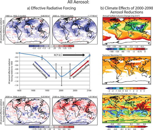
The spatially inhomogeneous distributions of aerosols and their RF, as compared to CO₂ and other well-mixed GHGs, can elicit different climate responses for the same global mean RF (e.g., Hansen et al., 2005; Shindell, 2014). Figure 4a illustrates spatial patterns of anthropogenic ERF for 1980 and 2000 relative to 1850, as well as for projections to 2030 and 2100 relative to 2000 (Shindell et al., 2013). The global anthropogenic aerosol abundance and ERF are projected to climax around present day. Continued reductions are projected for the 21st century (Figure 4a) under the RCP scenarios (see Emissions section above). These reductions are estimated to benefit human health (Silva et al., 2013), improve visibility, and lessen acid deposition. They would also lessen the net cooling influence that has slowed the increase in GMST induced by rising GHGs, and would reduce aerosol-induced perturbations of precipitation patterns. Figure 4b shows an example from one CCM in which anthropogenic aerosols are reduced, inducing surface warming (most locations in the Northern Hemisphere warm in summer by an additional 1°C, with some regions over 2°C) and changes in precipitation (particularly strong over Asia) by the end of the 21st century. The decrease in the sulfate burden in Figure 4b corresponds to the spatial pattern of ERF determined from the ACCMIP multimodel ensemble in Figure 4a, emphasizing the dominant role of anthropogenic sulfate in pre-industrial to present-day climate forcing, and its decline along the RCP scenarios.

Figure 4. Estimated climate forcing from aerosols at selected historical and future time periods, and an example of changes in climate by the 2090s due to aerosol reductions. (a) Global mean ERF (see Key Terms) relative to 1850 estimated from multimodel (ACCMIP CCMs) time slice simulations at 1930, 1980, 2000, 2030, and 2100. Also shown are the spatial patterns of all aerosol ERF at 1980 and 2000 relative to 1850, and at 2030 and 2100 under RCP8.5 relative to 2000. (b) Estimated impact on climate from 21st-century reductions in atmospheric aerosol abundances as projected by one CCM (GFDL CM3) for RCP4.5; SO₂ trends are similar to RCP8.5. Top panel: decrease in annual sulfate burden at the end of the 21st century. Middle and bottom panels: changes and temperature and precipitation, respectively, induced by the aerosol reductions. The changes in (b) are obtained by differencing a set of scenarios: One follows the RCP4.5 scenario for both GHGs and PM, and another holds PM and its precursors at 2005 levels but follows RCP4.5 for GHGs. White areas in the top two panels are where the difference between the two simulations is less than twice the standard deviation of annual variability in a control simulation (perpetual 1860 conditions). Adapted with permission from (a) Figure 18 of Shindell et al. (2013) in accordance with the license and copyright agreement of European Geosciences Union, and (b) Figure 6 of Levy et al. (2013) according to the license and copyright agreement of American Geophysical Union.

The climate impacts resulting from spatially inhomogeneous aerosol forcings can span local to global scales (Jacobson et al., 2007; Shindell and Faluvegi, 2009; Shindell et al., 2010; Ming et al., 2011; Leibensperger et al., 2012a; Levy et al., 2013). The spatial correlation between the change in sulfate column burden and the ultimate changes in surface air temperatures or precipitation is fairly weak (Figure 4b). Kloster et al. (2009) noted an amplified response of the hydrological cycle to changes in aerosols relative to GHGs. The climate effects of changes in domestic PM emissions may extend well beyond the jurisdiction of a given source region. Ganguly et al. (2012) and Bollasina et al. (2014) found that both local and remote aerosol sources have influenced the South Asian Monsoon, particularly precipitation in India, with the local aerosol source dominating the effect. Shindell and Faluvegi (2009) and Shindell et al. (2010) found that mid-latitude aerosol RF influences climate on a global scale, with a particularly large effect on the Arctic.

In the following, we summarize the RF, ERF, and climate impacts of the major anthropogenic aerosol components. Aerosol formation, removal, and natural sources are expected to respond to climate (Figure 2), and we discuss specific processes in Supplemental Text S4.

Sulfate

Sulfate aerosols form through SO₂ oxidation in both gaseous and aqueous phases. Sulfate contributes most to the cooling component of anthropogenic aerosol RF, with an IPCC AR5 RFari of –0.4 [5–95% uncertainty range is –0.6 to –0.2] W m⁻² (Myhre et al., 2013a; Figure 1), consistent with more recent estimates (e.g., Li et al., 2014; Heald et al., 2014; Zelinka et al., 2014). Sulfate also plays a dominant role in anthropogenic aerosol–cloud interactions (Takemura et al., 2012; Shindell et al., 2013). Zelinka et al. (2014) estimate a total ERF (ERFari + ERFaci) for sulfate of –0.98 W m⁻², which is 84% of their estimate for net forcing from all aerosols.

Anthropogenic sulfate is most concentrated in the mid-latitudes of the Northern Hemisphere where anthropogenic SO₂ sources are largest. This nonuniform forcing distribution creates a hemispheric disparity in cooling that can alter the large-scale atmospheric circulation. Sulfate cooling of the Northern Hemisphere has been hypothesized to shift the Intertropical Convergence Zone (ITCZ) southward (Hwang et al., 2013). The ITCZ is the principal tropical band of precipitation, and a southward shift may have contributed to the Sahel drought (Biasutti and Giannini, 2006; Giannini et al., 2008; Ackerley et al., 2011) and influenced the frequency of hurricanes (Merlis et al., 2013). Within the Northern Hemisphere, sulfate cooling is largest in the mid-latitudes (~40° N) and may induce a southward shift of the jet stream (Rotstayn et al., 2014). Shifts in the jet stream have large ramifications, including for air pollution, given their association with the trajectory and intensity of mid-latitude storm systems that ventilate the polluted boundary layer. Sulfate cooling has also been found to influence precipitation within mid-latitude storms (Igel et al., 2013; Thompson and Eidhammer, 2014), the intensity of the Pacific storm track (Wang, Yuan et al., 2014), the southward shift of precipitation in eastern China (Wang et al., 2013), spatial shifts in large-scale and convective precipitation in northeastern North America (Mashayekhi and Sloan, 2014), and precipitation and lightning within supercell thunderstorms (Morrison, 2012; Mansell and Ziegler, 2013; Kalina et al., 2014).

The cloud-albedo effect, which is dominated by sulfate in current models, depends on assumed preindustrial abundances (Carslaw et al., 2013) due to the logarithmic relationship between aerosol number concentration (number of particles per volume) and cloud droplet number concentration (number of cloud droplets per volume). This nonlinear dependence leads to a plateau in the concentration of cloud droplets as aerosol abundances increase. Stevens (2013) suggested that the cloud-albedo effect is now irrelevant since its magnitude may have leveled off in the 1980s despite continued increases in the global aerosol burden (Carslaw et al., 2013). This view, however, ignores the continuing effect of fine PM reductions in North America and Europe since the 1980s (see previous section). While trends vary by region, global emissions of SO₂ declined by 2010 to a level not seen since the 1960s (Klimont et al., 2013; Smith et al., 2011). Moreover, the RCP scenarios project SO₂ emissions nearing preindustrial levels by the end of the 21st century (Figure S2). Such large changes could lead to CCN also reverting to near preindustrial levels, unleashing additional unmasking of GHG warming. Observed decreases in aerosols (Murphy et al., 2011; Leibensperger et al., 2012b; Keene et al., 2014) have apparently already produced near-term climate impacts. Leibensperger et al. (2012a) attributed a portion of the rapid warming in the U.S. during the 1980s to reductions in the cooling influence of sulfate aerosols.

Nitrate. Nitrate aerosol forms via oxidation of NO_x, but it is closely coupled to sulfate because of their shared interaction with ammonia and interdependence through aerosol thermodynamics, which favors formation of ammonium sulfate over ammonium nitrate. Nitrate aerosol formation requires the presence of ammonia to neutralize gaseous nitric acid and form ammonium nitrate particles (Seinfeld and Pandis, 2006; Pinder et al., 2007; Pinder et al., 2008). The lifetime of nitrate is usually shorter than sulfate due to its high volatility (high temperatures favor the gas phase). The RFari of nitrate is estimated at –0.11 [–0.3 to –0.03] W m⁻² (Boucher et al., 2013; Figure 1), but may become increasingly important as decreasing SO₂ emissions lower the sulfate demand on ammonia, enabling increased (ammonium) nitrate formation (Bauer et al., 2007; Bellouin et al., 2011; Hauglustaine et al., 2014). The magnitude of nitrate changes, however, varies by region (Blanchard et al., 2007) and with PM composition (Ansari and Pandis, 1998), which could result in minimal nitrate compensation of sulfate decreases. Differing seasonal cycles of sulfate (greatest in summer) and nitrate (greatest in winter) also complicate nitrate compensation. Nitrate RF was not included in most of the ACCMIP models, but two project an increase, while one indicates little change (Shindell et al., 2013).

Black carbon (BC)

The primary source of BC is inefficient combustion of carbon-containing fuels (Table 2). BC absorbs sunlight, exerting a positive RF, which warms the atmosphere. Current knowledge of emissions, RF, and climate impacts was summarized by Bond et al. (2013) and EPA (2012). IPCC AR5 estimates a BC RFari for anthropogenic fossil fuel and biofuel use of +0.4 [+0.05 to +0.8] W m⁻² (Boucher et al., 2013; Figure 1), which is a compromise between a lower value from the AEROCOM II model intercomparison (+0.23 W m⁻²) (Myhre et al., 2013b) and the higher value from Bond et al. (2013) (+0.51 W m⁻²). IPCC AR5 estimates additional contributions of +0.2 W m⁻² from biomass burning sources and +0.04 W m⁻² from BC deposited on bright snow and ice surfaces (Myhre et al., 2013a), yielding a total of +0.64 W m⁻² (Figure 1). Rapid adjustments are particularly important for BC, which extend the fossil fuel, biofuel, and biomass burning BC RFari (+0.71 W m⁻²) of Bond et al. (2013) to an ERFari + ERFaci of +1.1 [+0.17 to +2.1] W m⁻², largely through cloud modifications (+0.23 [–0.47 to +1.0] W m⁻²) and changes in surface albedo (+0.10 [+0.014 to +0.30] W m⁻²). We discuss below the uncertainties in estimating BC ERFari and ERFaci.

The RFari from BC is sensitive to its vertical profile (Samset et al., 2013) and the assumed mixing state of aerosol particles (Jacobson, 2000). Chemically inactive, BC can acquire coatings of hydrophilic gases and aerosol species that generally scatter sunlight, including sulfate and some organic aerosol, as it ages. The absorption cross section of BC particles increases with this coating and the surface scattering components focus sunlight into the BC core, enhancing absorption (“lensing effect”). Estimates of BC RFari can differ by up to 0.5 W m⁻² depending on BC mixing-state assumptions (Klingmüller et al., 2014). Observations indicate that accurate representation of hydrophilic coatings of BC, and of the time scale for their accrual, is critical in determining the atmospheric lifetime of BC against wet deposition, the dominant BC sink (Jacobson, 2012; Wang X. et al., 2014, and Wang Q. et al., 2014). Models including these processes better match remote aircraft observations, and suggest revising downward the RFari from BC by as much as 25% (Samset et al., 2014; Wang, X. et al., 2014; Wang, Q. et al., 2014).

BC and BrC (see OC section) have an additional indirect forcing pathway following their removal from the atmosphere: deposition onto bright snow and ice surfaces, which decreases surface albedo and increases absorption of incoming sunlight (Figure 3). If the presence of BC induces melting that reveals underlying dark ground or ocean surfaces, there is an additional forcing adjustment that constitutes a positive feedback. Myhre et al. (2013a) and Bond et al. (2013) estimate this pathway to contribute a global mean ERFari (which includes the rapid adjustments from cryospheric or land-surface feedbacks triggered by the deposited BC) of +0.10 [0.014 to 0.30] W m⁻².

By serving as IN, or CCN if sufficiently coated in hydrophilic material, BC modifies ice, mixed-phase, and liquid clouds, but the magnitude and sign of these effects are uncertain. BC induced atmospheric warming can evaporate cloud droplets, “burning off” the cloud (semidirect effect; Figure 3). This alters precipitation and reduces cooling from clouds. For example, Panicker et al. (2014) observed less cloud liquid water and increased absorption of solar radiation in BC-polluted cloud layers in northeast India than in cleaner cloud layers. BC absorption is enhanced when it serves as a CCN, due both to a lensing effect and to scattering cloud particles that focus sunlight on a BC particle within a cloud. Cloud absorption effects are potentially a large positive RF (Jacobson, 2012, 2014). Bond et al. (2013) estimate radiative effects of BC (including the semidirect effect) on liquid clouds to be –0.1 [–0.3 to +0.1] W m⁻², on mixed-phase clouds to be +0.18 [0.0 to +0.36] W m⁻², and on ice clouds to be 0.0 [–0.4 to +0.4] W m⁻², based upon two, three, and two modeling studies, respectively.

The eventual, net climate effect of BC is surface warming (Wang, 2004; Hansen et al., 2005; Chung and Seinfeld, 2005; Jones et al., 2007; Koch et al., 2009b; Jacobson, 2010), even though the local surface directly beneath BC cools initially. BC is generally found to decrease precipitation (Figure 3), reflecting the net sum of two opposing influences: atmospheric heating aloft versus BC-induced surface warming, which would tend to increase precipitation (Andrews et al., 2010; Ming et al., 2010; O’Gorman et al., 2012). BC has been tied to a stronger temperature response at northern mid-latitudes (Shindell and Faluvegi, 2009), regional northward shifts of the ITCZ (Wang, 2007), and expansion of the tropical zone (Allen et al., 2012). Large sources of BC in India and China likely influence the Asian monsoon (Menon et al., 2002; Meehl et al., 2008; Randles and Ramaswamy, 2008; Wang et al., 2009; Bollasina et al., 2011; Ganguly et al., 2012; Bollasina et al., 2014).

Organic carbon (OC)

The IPCC AR5 estimate for organic aerosol (primary and secondary) RF is –0.12 [–0.4 to +0.1] W m⁻² (Boucher et al., 2013; Figure 1). OC includes aerosols from both primary combustion sources, which are largely the same as for BC, and secondary organic aerosols (SOA) formed from natural and anthropogenic organic precursor emissions (Lambe et al., 2013). Both primary and secondary sources can include partially absorbing components, collectively termed brown carbon (BrC; see also Supplemental Text S4).

New techniques are improving measurements of speciated OC and total carbon (Turpin et al., 2000; Chow et al., 2005; Goldstein and Galbally, 2007; Chow et al., 2011; Chen et al., 2014), crucial for source apportionment and identifying the chemical mechanisms leading to SOA formation (Carlton et al., 2009; Aumont et al., 2012; Zhang and Seinfeld, 2013). Models typically underestimate organic aerosols (Heald et al., 2005), but consideration of aqueous cloud processing (of isoprene oxidation products; e.g., Lim et al., 2005; Carlton et al., 2007; Ervens et al., 2008) improves model–observation comparisons (Carlton et al., 2008; Fu et al., 2008), and these processes are beginning to be incorporated into the models in Table S1 (He C. et al., 2013). Additional SOA formation pathways occur on aqueous aerosols (e.g., McNeill et al., 2012; McNeill, 2015) and may depend on anthropogenic sulfate via aerosol liquid water (Carlton and Turpin, 2013), but many of these processes are not yet included in the models used to estimate climate forcings.

The AeroCom models attribute –0.03 [–0.04 to –0.01] W m⁻² of the OC RF to biofuel and fossil fuel sources and another –0.06 [–0.15 to +0.03] W m⁻² from biomass burning (Myhre et al., 2013b). The IPCC AR5 estimates SOA RF to be –0.03 W m⁻², with a wide 90% confidence interval (–0.27 to +0.20 W m⁻²); SOA increases since the preindustrial era reflect enhanced partitioning of biogenic precursor gases to anthropogenic particles and oxidation changes associated with anthropogenic activities (Myhre et al., 2013a; see their Table 8.4). The large, but uncertain, biogenic fraction of OC complicates RF estimates, especially for aerosol–cloud interactions due to the sensitivity to background levels of cloud droplet number concentration (Scott et al., 2014).

The absorbing component of OC, BrC, is neglected in many models. Observations over California indicate that BrC absorption is 20–40% that of measured elemental carbon (Bahadur et al., 2012; Chung et al., 2012), which peaks in summer with SOA production and forest fire frequency (Bahadur et al., 2012). Smog chamber experiments indicate that BrC from biomass burning depends mainly on burn conditions, and can be parameterized as a function of BC to organic aerosol ratios (Saleh et al., 2014). Woo et al. (2013) suggest that secondary BrC forms through aqueous chemistry in aerosol and cloud droplets. X. Wang et al. (2014) used AERONET AAOD (aerosol absorption optical depth) and in situ observations to conclude that BrC absorption has been incorrectly attributed to BC, and that BrC contributes an RF of +0.11 W m⁻². Aircraft observations over the U.S. reveal BrC throughout the troposphere, increasing relative to BC with altitude, consistent with a free tropospheric, secondary BrC source (G. Lin et al., 2014). A large absorbing BrC component could cancel the scattering portion of OC, leaving the net forcing of BC plus OC aerosols roughly equal to the forcing of BC (Chung et al., 2012).

Attributing climate impacts to specific sectors

Thus far, we have focused on climate impacts resulting from perturbations to individual air pollutants (Figure 1), yet most sources emit more than one air pollutant. A single emitting source thus alters multiple atmospheric constituents, and each perturbation sets in motion a suite of climate responses. While some air pollution controls can remove a single pollutant from some sources (e.g., PM, NO_x, or SO_x from power plants), the current lack of widely applicable technology to prevent CO₂ release to the atmosphere means that controlling CO₂ emissions necessarily involves changes in co-emitted species by improving combustion, switching to less carbon intensive fuels, or switching to renewable energy sources. Consideration of the full suite of air pollution and climate implications when developing climate or air pollution strategies may help to maximize public health, climate, and other benefits, while guarding against unintended adverse consequences.

In a conceptual exercise, Unger et al. (2010) attributed climate forcing to specific economic sectors (Figure 5), illustrating the complexity introduced by considering co-emitted pollutants, a viewpoint absent from Figure 1. Adjoint methods (Table S1) offer an efficient approach to estimating RF for sectors or regions of interest (Henze et al., 2012), and complement the forward-model source perturbation approach of Unger et al. (2010). Figure 5 contrasts the temporal differences in RF from NTCFs versus CO₂. Sectors that warm near-term climate (2020; Figure 5a) the most include high-CH₄ emitters (animal husbandry and waste/landfill sectors) or BC-rich emitters (on-road vehicles and household biofuel and household fossil use). For long-term climate warming (2100; Figure 5b), the energy sector becomes the major player with its high CO₂ emissions, followed by road vehicles. Industry switches from inducing a strong net cooling in 2020 to a strong net warming by 2100 as the negative RF due to short-lived sulfates (and associated aerosol–cloud interactions) is overwhelmed by CO₂ RF in the long term (Figure 5a vs. Figure 5b). For BC, lowering emissions from “BC-rich” sectors including diesel engines and household biofuel and fossil-fuel use appears more likely to offer climate benefits than reducing biomass burning (Bond et al., 2013; Unger et al., 2010; Figure 5). Thus, continued BC emissions reductions from diesel PM regulations, widely adopted in the developed world are likely to produce a near-term climate benefit (EPA, 2012; Ramanathan et al., 2013).

Figure 5. Illustrative approach comparing RF contributions by species from 13 major anthropogenic emission sectors with perpetual year 2000 emissions by (a) 2020 and (b) 2100, adapted with permission from Figure 1 of Unger et al. (2010). The RFs from O₃ and PM and their precursors are estimated using a CCM, while the RFs from CH₄, nitrous oxide (N₂O), and CO₂ are estimated with a reduced complexity climate model (Table S1). The net RF is shown next to each sector. Reductions in emissions from sectors with positive RFs will produce a climate cooling, and vice versa. The RF from individual atmospheric constituents is shown in color, for example, of BC-rich sectors as household biofuel, and on-road transportation (largely from diesels). AIE denotes aerosol–cloud interactions formerly referred to as the aerosol indirect effect (Figure 3). Sector rankings (from strongest warmers to strongest coolers) change from near-term (a) to long-term (b) due to different atmospheric lifetimes of species. Uncertainties in these estimates reflect poorly bounded emission magnitudes including for cooling versus warming agents and naturally arising climate variability, and are largest for household fossil fuel and biofuel, off-road (land) transportation, shipping, biomass burning, and agricultural waste burning.

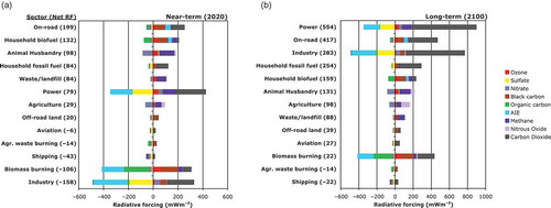
Figure 5 reveals opposite-signed RF from aerosol-cloud interactions, with warming attributed to BC-rich sources but cooling attributed to sulfate-rich sources. This result stems from different cloud responses to BC versus sulfate, all of which are highly uncertain (for more detail see Jacobson, 2012; Bond et al., 2013; Boucher et al., 2013). Jacobson (2014) suggests that the net negative forcing for biomass burning in Figure 5a may be incorrect, in part due to BC cloud absorption effects, and to other factors such as BrC neglected in prior estimates, which combined might lead to a net warming on a 20-year time scale.

Several studies examine the impact of the aviation sector on atmospheric composition and climate (Holmes et al., 2011; Unger, 2011; Köhler et al., 2013; Olsen et al., 2013). Aviation NO_x exerts a stronger impact on climate than equivalent NO_x emissions from surface sources (e.g., Wild et al., 2001; Unger, 2011), and even these vary as a function of latitude, with larger impacts at lower versus higher latitudes (Köhler et al., 2013). Figure 5 suggests aviation switches sign from near- to long-term as warming from CO₂ outweighs the near-term cooling from sulfate and the decrease in CH₄ associated with NO_x emissions, though the net RF is small relative to other sectors (Figure 5; Holmes et al., 2011).

Emissions from the agricultural and animal husbandry sectors are projected to increase over the 21st century as population grows. Decreasing CH₄ emissions from these sectors (Figure S2) could lessen near-term warming, while reducing the associated N₂O would lessen long-term warming (Figure 5), as well as helping meet stratospheric O₃ objectives (Ravishankara et al., 2009). Several studies project an increase in global nitrate aerosol over the 21st century as SO₂ emissions decline while NH₃ emissions from agricultural sources rise (Liao and Seinfeld, 2005; Bauer et al., 2007; Pye et al., 2009, Bellouin et al., 2011; Hauglustaine et al., 2014). Preventing growth in NH₃ could thus help maintain some of the air quality benefits attained from controlling SO_x (e.g., Lehmann et al., 2007; Leibensperger et al., 2012b), along with the climate disbenefits. Emissions of NH₃ and CH₄ from the agriculture, animal husbandry, and waste/landfill sectors, however, are poorly quantified (e.g., Pinder et al., 2006; Dlugokencky et al., 2011; Kirschke et al., 2013; Matthews, 2012). Measurements from field campaigns targeting regions heavily influenced by agriculture (Ryerson et al., 2013) and from satellite-based instruments that can provide a global picture of NH₃ (e.g., Shephard et al., 2011; van Damme et al., 2014) and CH₄ (e.g., Frankenberg et al., 2008; Bloom et al., 2010; Wecht et al., 2012; Turner et al., 2015) offer the potential to advance our understanding of emissions from these sectors. Wecht et al. (2014a) demonstrate the potential for space-based instruments to provide spatially detailed information within a region (California). The long-term remote network measuring CH₄ is invaluable for tracking global CH₄ changes and bounding the total emissions (e.g., Dlugokencky et al., 2003; 2009) but needs extension to bound regional or sectoral emissions (Dlugokencky et al., 2011). Isotope measurements offer promise for distinguishing among CH₄ sources (e.g., Mikaloff Fletcher, 2004a, 2004b; Monteil et al., 2011).

The broad definitions of the economic sectors in Figures S2 and 5 do not provide information as to the impacts from specific practices within a sector that may change the mix of emitted species. For example, a switch from entirely coal-based power generation to entirely natural gas within the energy sector would reduce CO₂ and sulfates, but net CH₄ emissions might rise if there is substantial leakage in the production and distribution of natural gas that outweighs the decline in CH₄ release from reduced coal mining (Wigley, 2011). While the reduction of sulfate is beneficial to health and welfare, it accelerates near-term warming (e.g., Wigley et al., 2009), as would any additional CH₄ released to the atmosphere. To assess the climate impacts from fuel transitions, Alvarez et al. (2012) propose a new “technology warming potential” that extends the global warming potential (GWP; see Key Terms and Table 2), considering only CO₂ and CH₄, to include the impacts from changes in the dominant fuel used for energy production or transportation. A more complete metric would include NTCFs such as SO_x and BC (Table 2). The utility of metrics to gauge the impacts of changing technological (or agricultural) practices is, however, limited by the credibility of emission estimates.

Accordingly, determining whether U.S. oil and gas operations, including expanded hydraulic fracturing, are in fact releasing much larger amounts of CH₄ to the atmosphere than expected based on older inventories has commanded attention (Brandt et al., 2014). Observational analyses find that emission inventories underestimate U.S. CH₄ emissions, particularly those from fossil fuel extraction and refining (Pétron et al., 2012, 2014; Peischl et al., 2013; Karion et al., 2013; Miller et al., 2013; Kort et al., 2014). An aircraft campaign over southwestern Pennsylvania suggested that shale gas wells in the drilling phase were leaking CH₄ emissions at 2–3 orders of magnitude greater than that estimated by EPA (Caulton et al., 2014). Space-based remote sensing supports these conclusions, indicating leakage rates of ~10% over the Bakken and Eagle Ford shale plays, rates sufficiently high as to call into question the climate benefits of switching from coal to gas (Schneising et al., 2014). Collectively, these observations suggest an upward revision of current estimates of CH₄ release from oil and gas production is needed. Wecht et al. (2014b) find that satellite-inferred CH₄ emissions suggest little need to revise the overall U.S. oil and gas emission budget, but that the livestock source requires upward revision, also noted by Miller et al. (2013). Measurements are crucial to validate the emission inventories used in life-cycle assessments of changes in GHG emissions resulting from fuel switching within the energy sector (e.g., Burnham et al., 2011).

Concerns have been raised as to the air pollution impacts from oil and gas operations (e.g., Litovitz et al., 2013). High wintertime O₃ episodes over snow-covered western U.S. oil and gas fields have been observed (e.g., Pinto, 2009; Schnell et al., 2009). Analysis of measurements during wintertime field campaigns indicates that snow-covered ground enhances photolysis rates to drive rapid O₃ production from the extremely high NMVOC present alongside NO_x in oil and gas fields (Edwards et al., 2014). Under strong wintertime temperature inversions, O₃ produced photochemically in this manner can accumulate to high concentrations (Edwards et al., 2014).

Climate Influences on Ground-level O₃ and PM_2.5

Local to regional weather determines pollutant transport into, within, and out of a given region, while also influencing atmospheric chemistry and emissions. We examine here the responses of ground-level O₃ and PM_2.5 to regional climate. These responses include changes in natural emissions, which not only influence local air quality but may also change global atmospheric composition, and thus climate forcing (Figure 2), serving as a feedback to the climate system (Supplemental Text S4). While mercury, persistent organic pollutants, and other air toxics are expected to respond to changes in regional climate (see Jacob and Winner, 2009; TF HTAP, 2010b, 2010c), we retain our focus on O₃ and PM_2.5 because of their two-way interaction with the climate system described earlier.

The influence of meteorology on air pollution poses two challenges to air quality management. First, variations in weather on weekly to annual scales introduce an uncontrollable random component that can mask the true efficacy of air quality improvement strategies in the short-term (Gégo et al., 2007). Second, climate change can alter regional meteorology conducive to pollutant buildup, imposing a “climate penalty” (see Key Terms) or, for example, can enhance ventilation of the polluted boundary layer, yielding a “climate benefit” (e.g., Trail et al., 2013). A quantitative understanding of how air pollution meteorology responds to climate change and natural variability is needed to inform air quality planning and regulation accountability for the coming decades (Ravishankara et al., 2012; Dawson et al., 2013).

Studies documenting strong correlations between individual meteorological variables and ozone or PM_2.5 were reviewed by Jacob and Winner (2009), and updated by Fiore et al. (2012) and Kirtman et al. (2013). Collectively, these studies constitute a strong line of evidence documenting the potential for changes in regional air pollution meteorology to alter air pollution levels. Historically observed relationships between relevant meteorological variables and O₃ (e.g., Bloomer et al., 2009; Lin et al., 2001) and PM_2.5 (e.g., Tai et al., 2010; Dawson et al., 2013) provide tests for model responses to regional climate variability and change (Rasmussen et al., 2012; Brown-Steiner et al., 2015). CCMs used to project the response of air pollution to changes in climate should accurately represent these present-day relationships (Supplemental Text S5). Applying local observed relationships for statistical downscaling of future air pollution responses to climate change could lead to inaccurate projections when individual meteorological–chemical relationships reflect a common underlying driver such as synoptic meteorology (e.g., the nonstationary temperature–O₃ relationship in Figure 6 and Supplemental Text S6).

Figure 6. Covariance between O₃ and temperature as measured at the Pennsylvania State Clean Air Status and Trends Network (CASTNet) site in Pennsylvania (41º N, 78º E, 378 m). (a) July mean maximum daily 8-hr average (MDA8) O₃ (black line and circles; left axis) and July mean daily maximum temperature (red line and triangles; right axis) from 1988 to 2014. (b) Scatterplot of the time series in (a) for 1988–2001 (black) and 2002–2014 (red); ordinary least squares slopes and correlation coefficients are shown, illustrating the shift after 2002 induced by regional NO_x emission controls (Bloomer et al., 2009). A color version of this figure is available online.

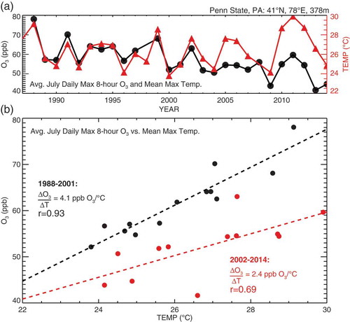
An important component of air pollution meteorology is the ventilation and dilution of a pollutant from its source, which often correlates with temperature and humidity in synoptic weather systems. The rate of ventilation is governed by wind speed, direction, and mixing height (vertical extent of surface air mixing): faster winds in a deeper mixed layer rapidly disperse and dilute pollutants. Shallow mixed layer depths and low wind speeds restrict vertical motion, trapping air close to the surface and raising near-surface pollutant concentrations. The covariance of a pollutant with mixing depth, however, depends on its vertical profile. For example, free tropospheric O₃ concentrations generally increase with altitude, implying that a deeper mixed layer will mix O₃-rich air to the surface, as is suggested to occur at high-altitude western U.S. regions (Zhang et al., 2014).

PM_2.5 is affected by precipitation as well as ventilation and mixing, as most components are soluble and undergo wet deposition (in contrast to O₃ and some of its precursors). Regional changes in precipitation influence the spatiotemporal patterns of both fine and coarse particles (Jacob and Winner, 2009, and references therein), and levels of most PM_2.5 components correlate negatively with precipitation (Tai et al., 2010). Forecasting the effects of anthropogenic climate change on regional precipitation is subject to major uncertainties (Deser et al., 2012; Deser et al., 2013; Melillo et al., 2014), reflecting notoriously noisy (i.e., subject to large internal variability) and model-dependent projections (Supplemental Text S2). Multiple GCM projections indicate that 21st-century warming will increase winter and spring precipitation over the northern U.S. (Supplemental Text S2). In some regions, changes in precipitation frequency may be most relevant for projecting changes in PM_2.5 (Jacob and Winner, 2009; Fang et al., 2011).

Individual meteorological parameters with physical and quantifiable relationships to air quality include temperature (Bloomer et al., 2009; Day and Pandis, 2011), humidity, cloud cover, wind speed and direction (Dawson et al., 2007a, 2007b; Kleeman, 2008), boundary-layer depth, and precipitation (Dawson et al., 2013). Changes in these parameters, which tend to vary together on synoptic time scales (days to 1–2 weeks; Tai et al., 2010), alter the propensity for pollutant accumulation within the planetary boundary layer, as well as for secondary formation and removal. Eastern U.S. air pollution episodes commonly develop under the warm, cloud-free, and stagnant conditions of summertime high-pressure systems (Logan, 1989; Vukovich, 1995; Hegarty et al., 2007) and terminate with a passing convective storm or cold front (Cooper et al., 2001; Leibensperger et al., 2008). Daily to weekly variation in air pollution meteorology is thus driven by the fluctuation between low- and high-pressure systems. The relationship between air pollution and individual meteorological variables is inflated through covariation on synoptic time scales.

The worst air pollution episodes in the eastern U.S. occur under stagnation events in which stalled high-pressure systems create prolonged periods of light winds, clear skies, and high temperatures. Stagnation events over the eastern U.S. commonly occur under westward excursions of the Bermuda High (Eder et al., 1993; Zhu and Liang, 2012) and North Atlantic atmospheric blocking events (Box 14.2 of Christensen et al., 2013). Figure 7 shows the progression of a June 2012 stagnation event over the eastern U.S., during which air pools and degrades air quality until a cold front arrives. Cold fronts lift warm surface air away from the surface and replace it with cool, clean air. The frequency of stagnation events and its inverse, the number of cold-front passages, are thus strong predictors of air pollution episodes. In lieu of cold fronts, the number of mid-latitude cyclones is commonly used (Leibensperger et al., 2008; Turner et al., 2013), because low-pressure systems are easier to identify and track in both observations and model data: A minimum of sea-level pressure is identified and followed throughout the life cycle of the cyclone. Mid-latitude cyclones migrate under the jet stream, suggesting that jet location may affect air quality, as has been found for decadal time scales (Barnes and Fiore, 2013). A few studies emphasize the role of synoptic meteorology in driving observed daily variations in PM_2.5, developing predictors that encapsulate changes in numerous meteorological variables (Appelhans et al., 2012; Tai et al., 2012a, 2012b). These statistical predictors are based upon the most frequent meteorological patterns, which resemble the stagnation–cold front progression just described (Tai et al., 2012a). As climate warms during the 21st century, the frequency of migratory cyclones over the northeastern U.S. declines in one CCM (Turner et al., 2013), broadly consistent with a multimodel analysis of 15 GCMs (Tai et al., 2012b).

Figure 7. Accumulation and ventilation of eastern U.S. pollution modulated by synoptic weather events. Maximum daily 8-hr average (MDA8) O₃ (top row), daily 24-hr average PM_2.5 (middle row) measured by the EPA Air Quality System, and sea-level pressure (SLP, bottom row) during a late June 2012 heat wave event, following Figure 1 of Leibensperger et al. (2008). On June 26, O₃ and PM_2.5 remain low as a high-pressure system begins to build in the Midwest behind a passing mid-latitude cyclone (low-pressure system). As the high pressure slowly migrates southeastward June 27–28, pollutants accumulate to maxima exceeding 90 ppb for MDA8 O₃ and 25 μg m⁻³ for 24-hr PM_2.5, degrading air quality. Relief arrives through ventilation by the cold front of a mid-latitude cyclone on June 29–30. SLP data are from the National Center for Environmental Prediction-Department of Energy Reanalysis 2, and synoptic analysis is based upon the NOAA Daily Weather Maps archive (http://www.hpc.ncep.noaa.gov/dailywxmap). A color version of this figure is available online.

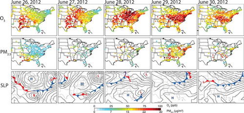
Climate change is expected to degrade air quality in polluted regions through unfavorable modifications to air pollution meteorology (Kirtman et al., 2013), particularly over the northeastern U.S. (Table S3), likely tied to a decline in the number of mid-latitude cyclones and the decrease in pollution ventilation by their associated cold fronts. Similarly, Horton et al. (2014) project increased stagnation affecting 55% of the global population with upward of an additional 40 days per year in the subtropics, and note a strong susceptibility to increased stagnation in the western U.S. A quantitative understanding of how air-pollution meteorology responds at the regional scale to both climate warming and variability could help to inform air quality planning for the coming decades.

U.S. Regional Air Quality Projections for the 21st Century

Anthropogenic and natural emission changes, as well as climate-induced changes in air pollution meteorology, will influence future air quality. In this section, we discuss projections for U.S. surface O₃ and PM_2.5 in response to climate change in the absence of emission changes, as well as in response to combined changes in climate and emissions, synthesized from various modeling studies. We show surface O₃ and PM_2.5 based on RCP projections from the ACCMIP and CMIP5 multimodel initiatives over seven U.S. regions with the regional boundaries used by Melillo et al. (2014). Finally, we address how natural climate variability confounds detection of regional climate change.

Impact of climate change on U.S. air quality

Numerous modeling studies offer initial insights into U.S. air pollution responses to changing climate or climate variability (Table S1), but there is little agreement across models, with regional changes often conflicting in sign (Figure 8). Changes in surface O₃ and PM_2.5 in the different U.S. regions attributed to climate change by various modeling approaches are compiled in Table S3 (column 5), for 2030, 2050, and 2100. Differences in modeling frameworks, including scenarios, simulation length, and the reported metrics, lead to a wide range in the estimated responses to climate change (Table S3). These studies show that at present-day emission levels, future climate change will degrade O₃ air quality over the U.S., especially over more polluted (high NO_x) areas, such as the U.S. Northeast, Southeast, Midwest, and southern California (Figures 8 and 9a; Gonzalez-Abraham et al., 2014, Hedegaard et al., 2013; Kelly et al., 2012; Trail et al., 2014; val Martin et al., 2015; Fann et al., 2015). An increase in pollution episodes in the eastern U.S. has been tied to decreasing numbers of summertime frontal passages (Mickley et al., 2004; Leibensperger et al., 2008; Tai et al., 2012a), which may in turn be associated with a northward migration of the mid-latitude jet stream (Barnes and Fiore, 2013).

Figure 8. Models indicate a climate penalty (see Key Terms) on surface O₃ over the northeastern U.S. but disagree over other regions. Simulated changes in summer mean MDA8 O₃ (ppb) in surface air in 2050 relative to 2000 under climate warming, holding O₃ precursor emissions constant at 2000 levels: (a) estimated with a GCM-CTM, the first to point out the climate penalty (reproduced with permission from Figure 2b of Wu et al. [2008a] in accordance with the license and copyright agreement of American Geophysical Union); and (b) regional spatial averages from seven models, each represented by an individual bar, with each group of bars representing one of (c) five U.S. regions. The Harvard model bars in (b) are derived from the simulation shown in (a). Panels (b) and (c) are reproduced from Figures 6 and 7a of Weaver et al. (2009). ©American Meteorological Society. Used with permission. A color version of this figure is available online.

Figure 9. Over the Northeastern U.S.A., NO_x emission reductions may guard against a climate penalty (see Key Terms) on MDA8 surface O₃ and may reverse the O₃ seasonal cycle; rising CH₄ induces a year-round O₃ increase, most pronounced in winter when the O₃ lifetime is longest. Simulated MDA8 surface O₃ (ppb) over the northeastern U.S. (36–46° N, 70–80° W; land only) averaged over 2006–2015 (black) and 2091–2100 (gray) in the GFDL CM3 CCM. (a) A regional warming of 5.5°C increases O₃ from May to September (gray vs. black triangles), diagnosed from a simulation in which well-mixed GHGs follow RCP8.5 but air pollutants are held fixed at 2005 levels (RCP8.5_WMGG; CH₄ follows RCP8.5 for climate forcing but is held at 2005 levels for chemistry). (b) Under the RCP8.5 scenario, CH₄ roughly doubles by the end of the century but NO_x emissions decline, decreasing O₃ during the warm season but increasing it during the cold season (black vs. gray circles). The NO_x emission reductions yield summertime O₃ decreases but wintertime increases, diagnosed with a sensitivity simulation in which CH₄ is held at 2005 levels but all other air pollutants and GHGs follow RCP8.5 (RCP8.5_2005CH₄; black vs. gray triangles). Doubling of global CH₄ partially offsets the warm season decrease and amplifies the winter–spring increase (gray circles vs. gray triangles). Symbols show decadal averages from individual ensemble members where available; lines show ensemble means. Adapted with permission from Figure S3 of Clifton et al. (2014) according to the license and copyright agreement of American Geophysical Union.

Of the three RCP scenarios considered in Table S3, the air pollution response is greatest for RCP8.5, the no-climate policy (highest RF) scenario. CCM, regional climate model (RCM)–regional chemistry–transport model (RCTM), and GCM–CTM studies suggest that the impact of climate change on U.S. surface O₃ predominantly occurs in summer, with increases of up to 9 ppb over the eastern U.S. (Figures 8 and 9a; Gonzalez-Abraham et al., 2014; Kelly et al., 2012; Trail et al., 2014; val Martin et al., 2015). Many of these studies, however, analyzed a single scenario of short simulation length such that some of this range may reflect climate variability rather than the anthropogenic climate change signal (see Supplemental Text S2 and below). Trail et al. (2014) find that MDA8 increases in spring in all but one of nine contiguous U.S. regions, and in autumn over the Pacific and Eastern regions, suggesting that climate warming lengthens the O₃ pollution season, consistent with Nolte et al. (2008) and Racherla and Adams (2008), and Figure 9a.

The response of PM_2.5 to climate change varies across modeling studies (Table S3), depending strongly on the simulated meteorology. Opposing influences of changes in temperature, precipitation, relative humidity, and stagnation on the individual PM_2.5 components and their chemistry confound a clean deciphering of PM_2.5 changes. Many studies neglect potentially important climate-induced changes in emissions from natural sources, such as increasing wildfires in the western U.S. Simulated climate warming leads to small increases in annual mean PM_2.5 in the northeastern U.S. through increased sulfate from SO₂ oxidation (Avise et al., 2009; Dawson et al., 2007b; Gonzalez-Abraham et al., 2014; Kelly et al., 2012; Trail et al., 2014) but there is no agreement on the magnitude. Trail et al. (2014) find that higher temperatures lower OC and ammonium nitrate particles by favoring gas-phase partitioning. Finally, couplings between anthropogenic and biogenic emissions occur; for example, initial estimates suggest that more than half of SOA derived from BVOC emissions may be controllable (e.g., Carlton and Turpin, 2013; Xu et al., 2015).

Impact of combined changes in climate and emissions on U.S. air quality

Projected changes in regional U.S. surface O₃ and PM_2.5 from combined changes in climate and emissions in 2030, 2050, and 2100 are summarized in Table S3 (column 6). The anthropogenic precursor emissions assumed in these studies usually follow either the SRES scenarios (e.g., Penrod et al., 2014) in which air pollutants and precursors span a wide future range, including increases (Prather et al., 2003), or RCP scenarios (e.g., Clifton et al., 2014) in which air pollutants and precursors decrease, with the exception of CH₄ in RCP8.5 (Figure S2; Table S4). Alternative lower air pollutant emission projections are also considered (Gonzalez-Abraham et al., 2014; Trail et al., 2014). A few studies estimate future climate-driven emission increases in U.S. PM or O₃ from biogenic sources, wildfires, or anthropogenic land use (e.g., Gonzalez-Abraham et al., 2014; Penrod et al., 2014; val Martin et al., 2015).

Stringent precursor emission reductions projected in the RCP scenarios (Figure S2) lead to summertime surface O₃ decreases over the U.S. throughout the 21st century (Table S3; Figures 9b and 10a; Clifton et al., 2014; Gao et al., 2013; Gonzalez-Abraham et al., 2014; Kelly et al., 2012; Pfister et al., 2014; Rieder et al., 2015; val Martin et al., 2015; Trail et al., 2014). These reductions in O₃ precursor emissions more than offset any climate penalty incurred from rising GHGs. Summertime O₃ air quality improves most over the eastern U.S., although the inter-model range is large (shaded region and vertical lines in Figure 10a). Across the majority of U.S. regions, O₃ decreases most under RCP2.6 and least under RCP8.5 as CH₄ increases, with the O₃ projections under the RCP2.6, RCP4.5, and RCP6.0 scenarios dominated by the projected regional NO_x (and other O₃ precursor) reductions (Figure S2). Trail et al. (2014) find little change in the sensitivity to NO_x in summer over the 21st century, consistent with the approximately linear dependence of various O₃ metrics on eastern U.S. NO_x emission changes found in one CCM (Rieder et al., 2015).

Figure 10. O₃ and PM air quality improves under the RCP scenarios, except that O₃ increases under RCP8.5 (reflecting the doubling of global CH₄), with little variation across the RCP scenarios despite a wider published range. Decreases are generally largest over the eastern U.S., where present-day anthropogenic emissions are largest. The figure follows those by Fiore et al. (2012) and Kirtman et al. (2013), and shows projected changes in (a) summer (June–July–August), (b) winter (December–January–February) mean surface O₃ (ppb mole fraction), and (c) annual mean surface PM_2.5 (μg m^–3 air; calculated as the sum of individual aerosol components except nitrate) from 1950 to 2100 following the historical (1950–2000) and RCP scenarios (to 2100) over seven contiguous U.S. regions defined in Melillo et al. (2014). The discontinuity at 2006 occurs because the precursor emission projections used by the CMIP5/ACCMIP models were not yet harmonized to base year 2000 levels. Results shown are averaged over each of the shaded regions. Continuous colored lines denote the average of 4 or fewer CMIP5 CCMs. Colored dots denote the average of 3, 9, 2, and 11 (or fewer) ACCMIP models for 2010, 2030, 2050, and 2100 decadal time slice simulations, respectively. The shading about the lines and the vertical bars on the dots represent the full range across models. Changes are relative to the 1986–2005 reference period for the CMIP5 transient simulations, and to the average of the 1980 and 2000 decadal time slices for the ACCMIP models. The average value and model standard deviation for the reference period is shown in each panel (CMIP5 models at upper left and ACCMIP models at upper right). A color version of this figure is available online.

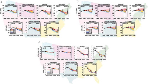
Both global and regional models project some regional wintertime O₃ increases, particularly in the northeastern U.S. and in metropolitan areas (e.g., Los Angeles, New York City), attributed in part to less O₃ titration by NO_x in winter (Gao et al., 2013; Clifton et al., 2014; Trail et al., 2014). Trail et al. (2014) note negative sensitivity of MDA8 to emissions of NO_x during fall, which indicates O₃ titration by NO_x over the northeastern U.S. in their regional model, consistent with the O₃ increases found in a CCM by Clifton et al. (2014) in nonsummer months (RCP4.5 and RCP8.5_2005CH₄ in Figure 9b). Under the RCP8.5 scenario, O₃ increases in winter (Figure 10b), spring, and fall, largely reflecting the high CH₄ levels that raise background tropospheric O₃ and the longer O₃ lifetime in the cold season (Figure 9b; Clifton et al., 2014; Gao et al., 2013; Pfister et al., 2014). Rising global CH₄ increases near-surface O₃ in nonsummer months and offsets some of the warm-season decreases attained with regional NO_x emission reductions, underscoring the combined air quality and climate benefits obtained via CH₄ emission reductions. Increasing foreign anthropogenic emissions of CH₄ and other O₃ precursors, which are challenging to project accurately, may also confound U.S. efforts to abate O₃ pollution (e.g., TF HTAP, 2010a), as would changes in U.S. biogenic sources or wildfires from either climate or land-use change (Gonzalez-Abraham et al., 2014; Pfister et al., 2014; val Martin et al., 2015).

The studies in Table S3 also project PM_2.5 decreases over most of the U.S. when climate warms but anthropogenic emissions of PM and precursors are reduced, with the strongest decreases over the eastern U.S., where SO₂ emissions were high in 1995–2004 but decline quickly during the 21st century (Figure S3; note the consistency with NO_x; Gonzalez-Abraham et al., 2014; Kelly et al., 2012; Penrod et al., 2014; Trail et al., 2014; val Martin et al., 2015). Global CCMs also project decreases in U.S. annual mean PM_2.5, largest in the eastern U.S., with little difference across the RCPs (Figure 10c). The PM_2.5 response to future climate and emission changes differs by U.S. region, reflecting variability in PM_2.5 composition. val Martin et al. (2015) and Spracklen et al. (2009) find that climate-driven increases in wildfire emissions enhance PM_2.5 concentrations over the western U.S. and Great Plains, a process absent from the projections in Figure 10c.

A few studies find that future eastern U.S. PM_2.5 will become more sensitive to changes in BVOC emissions, which influence SOA, induced by climate and land-use changes as NO_x and SO₂ are controlled (Gonzalez-Abraham et al., 2014; Trail et al., 2014). Several studies, however, emphasize the dependence of SOA formation on anthropogenic emissions, but mechanistic understanding is still developing (Hoyle et al., 2011; Carlton and Turpin, 2013; McNeill, 2015, and references therein). Reducing uncertainty in global modeling of SOA requires accurate emissions, reaction rates, and multiphase SOA formation mechanisms (Pye and Seinfeld, 2010; Spracklen et al., 2011). G. Lin et al. (2014) found that none of the multiphase SOA formation schemes implemented in a global model could represent all available observations, including over the U.S., China, and Europe. Therefore, it is not yet clear how SOA (and PM_2.5) will respond to concomitant anthropogenic emission controls, and climate and land-use driven changes in BVOC emissions.

In summary, models indicate that regional climate change and the processes it triggers (Figure 2) incur a climate penalty on surface O₃ over the northeastern U.S., but disagree over other regions. Continued efforts to reduce U.S. NO_x emissions should protect against this climate penalty. Scenario uncertainties (i.e., the projected trajectories for precursor emissions including CH₄) lead to a wide range of projected U.S. surface O₃ and PM_2.5 levels, and some regions are highly sensitive to changes in air pollutant emissions from the biosphere (e.g., wildfires in the western U.S., biogenic emissions in the eastern U.S.). Global CH₄ increases would raise U.S. background O₃, confounding efforts to reduce U.S. O₃ via regional precursor emission controls.

Influence of climate variability

Computational limitations have restricted the simulation length of many of the global and regional CTM and CCM studies in Table S1, with conclusions often based on 5 or fewer years of future versus present-day climate from a single realization from one climate model (Fiore et al., 2012, and references therein). Over these short simulation lengths, any meteorological changes may reflect internal variability that arises naturally in the chaotic climate system rather than a forced climate signal (Deser et al., 2012; Deser et al., 2013; Nolte et al., 2008; Supplemental Text S2). A major advance resulting from the growth in computational resources is the generation of “large ensembles” (i.e., differing only slightly in initial conditions) in a single climate model. Deser et al. (2012) used a 40-member ensemble with the NCAR climate model (CCSM3) to examine climate change and variability over North America under one climate change scenario (SRES A1B) and to illustrate the uncertainty inherent in any climate projection for the next several decades. Even on a 50-year time scale, trends in temperature and precipitation in many U.S. regions are subject to large uncertainties solely due to natural variability (Deser et al., 2012). By mid-century, model simulations with identical anthropogenic forcing generate U.S. temperature increases ranging from twice as large as the ensemble mean (4–5°C vs. 2–3°C) to <1°C over the Midwest; precipitation patterns conflict in sign over some regions between individual ensemble members and remain within natural variability over much of the central and mid-Atlantic U.S. (Deser et al., 2012).

The regional downscaling studies in Tables S1 and S3 thus depend crucially on their parent large-scale GCM, and often rely on a single ensemble member for a small number of years due to computational expense. While spatially refining the response of the GCM can be useful for decision making (Hall, 2014), the simulated regional climate change remains limited to a single realization out of a wide range of possibilities arising from natural variability. Detecting regional climate responses from changes in NTCFs is similarly confounded by internally generated climate variability, with more ensemble members or longer simulation periods needed to discern climate responses to smaller forcings.

An example of naturally arising climate variability is the El Niño Southern Oscillation (ENSO), whose frequency of occurrence is largely unpredictable and varies between decades and centuries (Wittenberg, 2009). Once an El Niño or La Niña event occurs in the tropical Pacific, however, well-established regional climate responses follow for precipitation, temperature, and circulation patterns associated with floods and droughts (the so-called “teleconnections”; Diaz et al., 2001; Goodrich et al., 2007). These atmospheric responses to climate variability induce changes in regional atmospheric composition (e.g., Langford et al., 1998; Koumoutsaris et al., 2008; Ziemke et al., 2010), including via dust events in the southwestern U.S. (Okin and Reheis, 2002) and wildfires in the northwestern U.S. (Hessl et al., 2004). Low-frequency variability (decadal time scales and longer) in natural climate fluctuations can confound the attribution of observed changes in chemical constituents to trends in emissions, as found for the 40-year tropospheric O₃ record at Mauna Loa, Hawaii (M. Lin et al., 2014).

Irrespective of whether the “forced” (anthropogenic) signal from climate change has been accurately quantified, the range of projections reported in Table S3 nevertheless provides a sampling of possible futures. Each individual projection reflects some combination of a forced regional climate signal, superimposed with internally generated climate variability. Barring a substantial change in the variance or shape of the distribution (as is expected from emission changes; see next section), observed year-to-year variability in air pollution (Leibensperger et al., 2008; Patz et al., 2014; Figure 6) provides a useful range for long-term planning. One study finds that rising background combined with a warming climate will increase the variance in future MDA8 U.S. surface O₃ (Pfister et al., 2014). Multiple studies find that, in the absence of U.S. emission changes, climate change will lead to a higher mean O₃ level, about which variations will occur, in at least some polluted U.S. regions (Figures 8 and 9a; Table S3). If the RCP-projected air pollutant emission reductions are realized, then mean U.S. pollutant levels will decrease (Figure 10), and the variance will shrink (e.g., Rieder et al., 2015; Pfister et al., 2014), as observed for O₃ in response to U.S. NO_x emission controls implemented in the 1990s and 2000s (Simon et al., 2014). Continued preparation for year-to-year fluctuations in regional air pollution associated with changes in weather should help to guard against the possibility of a climate penalty (EPA, 2014a).

Extreme O₃ and PM_2.5 Pollution

Any particular extreme event is influenced both by meteorological conditions and by the chemical and emission processes that respond to changes in meteorology (see earlier discussion and Supplemental Text 4). The most extreme O₃ events typically occur during heat waves, when abundant radiation facilitates photochemical production, including from temperature-sensitive biogenic and anthropogenic emissions, leading to accumulation in poorly ventilated near-surface air (National Research Council [NRC], 1991). The connection between extreme O₃ levels and extreme heat manifests as strong correlations in the number of days exceeding specific temperature and O₃ thresholds (e.g., Lin et al., 2001; Patz et al., 2014). Large events include the 2003 European heat wave (e.g., Ordóñez et al., 2005; Vautard et al., 2005; Tressol et al., 2008; Vieno et al., 2010) and the 1988 summertime eastern U.S. heat wave, a year with the largest number of O₃ episodes over this region (Lin et al., 2001). These individual events contribute to the observed year-to-year variability in monthly or seasonal averages (Fiore et al., 1998; Figure 6). Eastern U.S. NO_x emission control programs have alleviated some of the large-scale O₃ buildup during extreme heat wave events, as evidenced by the much smaller increase in July mean MDA8 O₃ in 2012 relative to 1988 as illustrated for one eastern U.S. site in Figure 6a (20 ppb lower despite hotter temperatures). While O₃ is still high in hot summers relative to cooler years, the enhancement of O₃ per degree of warming is lower as NO_x emissions decline (Figure 6b; Bloomer et al., 2009; Rasmussen et al., 2012).

Historically, the most extreme PM episodes have occurred during wintertime temperature inversions in which PM from inefficient coal combustion accumulated in a shallow boundary layer (e.g., the London fogs of the 1950s, and several U.S. cities in the 1940s–1960s; Bachmann, 2007). In China, recent wintertime inversions have led to PM_2.5 accumulation to levels of hundreds of micrograms per cubic meter (~25 times the U.S. daily standard; NASA, 2013). Accumulation of PM, albeit much lower than the historical U.S. events or current Chinese events, still occurs in the U.S. during wintertime inversions (Dawson et al., 2013). Residential wood burning in stoves and fireplaces contributes to peak daily PM_2.5 above the NAAQS level, particularly in the western U.S., New York, and New England. Dawson et al. (2013) find that air stagnation correlates with higher PM_2.5 levels year-round in Birmingham, AL,, and Tai et al. (2010) report a U.S.-wide average PM_2.5 increase of 2.6 μg m⁻³ on stagnant days.

In the absence of changes in other factors, warmer temperatures during stagnation episodes are expected to exacerbate peak pollution levels (IPCC, 2013c), through the mechanisms described in Supplemental Text S4. More heat waves are anticipated with climate warming, with the North American Regional Climate Change Assessment Program (NARCCAP) RCMs (Mearns et al., 2009, 2012) projecting increases of 25–50 days above 90°F (32.2°C) in much of the southern U.S. and of 10–25 days in much of the northern U.S. by 2041–2070 relative to 1971–2000 (Peterson et al., 2013). Increases in air stagnation events are projected as climate warms in many populated regions around the world, including within the U.S. during all seasons (Horton et al., 2012; Horton et al., 2014; Pfister et al., 2014), and imply a heightened susceptibility to pollutant accumulation.

Typical approaches to quantify extreme pollution events consider values at a specific high percentile (e.g., Wu et al., 2008a; Weaver et al., 2009) or the number of events above a fixed value that is considered extreme at present or relevant to attaining air quality standards such as the U.S. NAAQS (Lin et al., 2001; Lei et al., 2012; Rieder et al., 2015). Studies across a range of modeling platforms suggest larger increases of peak (typically 95th percentile) U.S. summertime MDA8 O₃ in response to regional climate warming, as compared to mean simulated increases (Jacob and Winner, 2009; Weaver et al., 2009; Fiore et al., 2012; Pfister et al., 2014; Trail et al., 2014), with one study specifically attributing increases in 95th percentile O₃ by the 2050s (up to a few ppb) to more intense heat waves (Gao et al., 2013). Large-scale extreme events occur under synoptic conditions (e.g., heat wave events) that are resolved even at the coarse scale of CCMs. Available studies provide strong evidence that the qualitative results from CCMs and CTMs are consistent with observations (Supplemental Text S5).

Wildfires and dust events can produce extreme PM levels that are typically classified as exceptional events (see next section). Yue et al. (2013) estimate that future increases in wildfires could enhance OC and BC levels above the 84th percentile by ~90% and ~50%, respectively, in Federal Class I areas within the Rocky Mountains, with associated decreases in visibility. Drought can also contribute to extreme dust events, particularly in regions with strong land-surface feedbacks; anomalously high dust loadings can in turn induce regional climate responses, exacerbating the drought, as may have occurred during the 1930s dust bowl (Cook et al., 2009). Variations of PM with drought conditions provide a means for improving process-level understanding of air pollution responses to climate variability, and the relative roles of various competing processes on the overall PM level. Wang Yuxuan et al. (2014) find a 26% increase in observed PM_2.5 over the southern U.S. from June 2010 to the June 2011 drought, mainly driven by higher OC from wildfires; they also find an 11% decrease over Texas due to less aqueous-phase sulfate formation as cloud cover decreased during the 2011 drought.

We highlight two new approaches to studying extreme pollution levels. The first systematically maps pollution episodes (MDA8 O₃) by considering the 10 most polluted days observed in each year from 2000 to 2009, corresponding to 97.3%, or the top 10% of events each summer (when most events occur) at each location on a 1° × 1° grid (Schnell et al., 2014). Schnell et al. (2014) find that O₃ episodes occur most frequently during June, with a peak in 2002, one of the warmest and most stagnant summers, with the fewest cyclone passages (Figure 9 of Leibensperger et al., 2008) over the northeastern U.S. for the 2000–2009 period considered. Schnell et al. (2014) also use their metric to evaluate the skill of global CCMs and GCM-CTMs in capturing the observed spatial extent (typically more than 1000 km) and duration of these O₃ extremes, including their regional migration over multiple days (e.g., Figure 7). This approach harnesses the strength of global CCMs and CTMs at capturing the synoptic, large-scale variability that drives the accumulation of pollutants (see Supplemental Text S5). This climatology describes the spatial extent and persistence of O₃ episodes, offering a benchmark against which to gauge changes, complementing the more common focus on their frequency and intensity (below).

The second approach characterizes the frequency and intensity of pollution episodes (MDA8 O₃) by applying extreme value theory statistical methods (Rieder et al. 2013). Figure 11 illustrates return levels (see Key Terms) for the “1-year” O₃ event over the eastern U.S. (probability of an event of that magnitude or higher occurring on 1 out of 92 summer days). The top two panels characterize air quality improvements in terms of declining 1-year return levels from the 1990s to the 2000s, estimated from decades-long observational records (Figure 11) and attributed to NO_x emission reductions (Rieder et al., 2013). The large NO_x emission reductions under RCP4.5 (Figure S2) yield lower 1-year return levels across the domain (Figure 11c), falling below 70 ppb by the 2030s and below 60 ppb by the 2060s (Figure 11e), levels that should attain compliance with proposed O₃ NAAQS levels, assuming high O₃ events occur in the summer season. In contrast, half of the domain is subjected to 1-year return levels above 75 ppb throughout the 21st century when the scenario is adjusted to hold regional O₃ precursor emissions constant (Figures 11d and 11f). The intensity of future O₃ pollution events thus depends on the anthropogenic emission scenario (see also Kirtman et al., 2013).

Figure 11. Extreme summer (JJA) MDA8 O₃ pollution levels in near-surface air over the eastern U.S. characterized in terms of 1-year return levels (see Key Terms) for 23 sites in the U.S. Clean Air Status and Trends Network (CASTNet) for (A) 1988–1998 and (B) 1999–2009. Also shown are 1-year return levels projected with a CCM (GFDL CM3; bias corrected as described by Rieder et al., 2015). Panels C and D show 1-year return levels at mid-century (2046–2055); panels E and F show 1-year return levels for each 21st-century decade, spatially averaged over the region in C and D. Following RCP4.5 (C and E), both air pollutant emissions and GHGs change, but under RCP4.5_WMGG (D and F), air pollutant emissions are held at 2005 levels while GHGs follow RCP4.5. Observed decreases in (B) relative to (A) are attributed to NO_x emission reductions (e.g., NO_x SIP Call) during this period; additional NO_x emission reductions projected under RCP4.5 (decreases of 60% by 2030, 75% by 2050, and 84% by 2100, relative to 2005 values over the eastern U.S.) produce even lower 1-year return levels in C and E. Increases in 1-year return levels induced by climate change are limited to a few ppb, with some regions experiencing decreases of up to a few ppb. (Rieder et al., 2015). Panels A and B are adapted from Figures 3a and 3c of Rieder et al. (2013) in accordance with the Creative Commons Attribution 3.0 Unported (CC-BY) license available at http://creativecommons.org/licenses/by/3.0; panels C, D, E, and F are adapted with permission from Figures 5c, 7b, 7b, and 8b, respectively, of Rieder et al. (2015), in accordance with the license and copyright agreement of American Geophysical Union. A color version of this figure is available online.

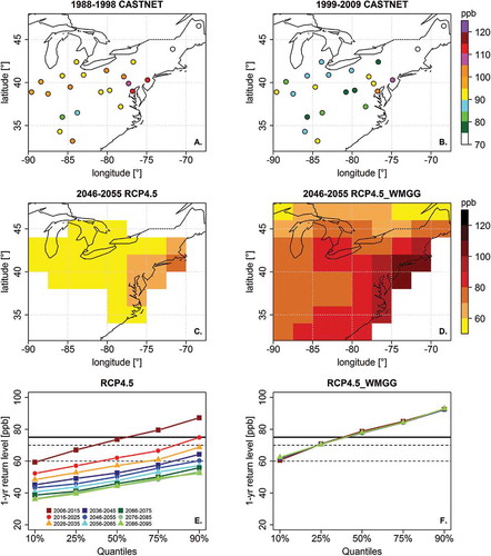
While the O₃ response to climate change shown in Figures 11d and 11f appears small in the context of the large projected emission changes under the RCP4.5 and other future scenarios (Prather et al., 2003; Fiore et al., 2012), it is not trivial. Increases and decreases of up to 4 ppb in 1-year return levels averaged across three available CCM ensemble members under the RCP4.5 scenarios occur by 2100 (Rieder et al., 2015). These changes are smaller than the upper end of the range reported in studies cited earlier, but this study more fully samples climate variability. Consideration of 30 years (10 years from each of three ensemble members), however, may yet be too small to quantify the anthropogenic climate signal (Deser et al., 2012).

Various factors can alter the frequency, intensity, and duration of O₃ and PM_2.5 extremes. When an extreme is defined relative to a standard concentration at present, for example, the 98th percentile in the daily PM_2.5 NAAQS, then its frequency of occurrence will change if there is a simple shift in the distribution to a higher mean state. A change in the width (variance) or shape (e.g., skewness) of the distribution will also alter the frequency of extremes. Understanding the factors shaping the overall pollutant distribution can thus help interpret changes in extreme concentrations. A mean shift could occur if baseline O₃ or PM_2.5 levels change. For example, changes in atmospheric CH₄ levels induce a mean shift in the U.S. near-surface summertime O₃ distribution in surface air (West and Fiore, 2005), a robust finding across models (Fiore et al., 2009). In contrast, NO_x emissions preferentially reduce the high tail of the summertime O₃ distribution in polluted regions (e.g., Fiore et al., 2002; West and Fiore, 2005; Rieder et al., 2015; Simon et al., 2014). Processes such as biogenic emissions, wildfires, deposition, and anthropogenic emissions associated with electricity generation are sensitive to daily weather fluctuations (Supplemental Text S4) and can amplify the high tail of the O₃ and PM_2.5 distributions.

Toward a Holistic Approach to Meeting Air Quality and Climate Goals

The multiple linkages between air pollution and climate (e.g., Figures 1 and 2 and Table 2) imply that their joint consideration would increase benefits to public health and the environment, while reducing unintended adverse impacts (e.g., Ramanathan and Xu, 2010). In light of the substantial estimates of adverse health impacts around the globe, emission controls on SO₂, BC, and O₃ precursors may continue to be imposed irrespective of climate policy (Smith et al., 2014; Anenberg et al., 2010; Silva et al., 2013). Changes in these NTCFs may alter near-term warming rates, as well as precipitation and regional circulations that affect the buildup of pollution. Avoiding disbenefits to air pollution from climate change requires additional controls on regional air pollutant and precursor emissions. While lessening any climate penalty, CO₂ reduction programs may also yield co-benefits to air quality by decreasing co-emitted air pollutants (e.g., West et al., 2013; Thompson et al., 2014). Not all climate mitigation strategies, however, improve air quality (e.g., Jacobson, 2007). Developing a more robust and quantitative scientific understanding about these connections—as well as about other environmental impacts—can help to reduce inadvertent undesirable consequences. In the following, we review recent research that aims to quantify the potential for SLCP reductions to lessen near-term warming, as well as the increase in near-term warming associated with anticipated reductions of cooling PM components. We also highlight growing challenges to U.S. air quality management from the rising relative importance of background levels for attaining U.S. air quality standards and provide some recommendations for research directions to support a more holistic approach to climate and air quality management.

Impacts of air pollution control strategies on climate

Reducing PM_2.5 or tropospheric O₃ requires a multipollutant approach (e.g., Hidy and Pennell, 2010), due to the various chemical classes that comprise fine particles, and the multiple O₃ precursors (Figure 2). The available evidence indicates that reducing atmospheric CH₄ is likely to benefit climate and improve O₃ air quality, while sulfate reductions reflect a trade-off between climate and air quality goals. Reducing BC and OC would yield global public health benefits (Anenberg et al., 2012), particularly from decreasing residential fuel use (Smith et al., 2014), and may reduce near-term RF, in contrast to decreases in major SO_x sources. The net climate impact from BC (and BrC) sources is more uncertain due to co-emitted OC, with reductions in BC-rich diesel engines and kerosene lamps, followed by residential fuel use, most likely to reduce near-term RF (Lam et al., 2012; Bond et al., 2013). A strong scientific understanding of the implications of these health-motivated emission changes for the climate system is needed to underpin a holistic approach to environmental management. The majority of studies investigating the potential role of SLCP reductions as a supplement to strategies for CO₂ and other long-lived GHG examine targets such as limiting peak warming and near-term warming rates of GMST. Climate goals, however, might also include reducing anthropogenic disruption of the hydrological cycle and the cryosphere.

Projected 21st-century changes in NTCFs and implications for GMST

Table S4 summarizes 21st-century RF projections for selected NTCFs under a stringent climate policy scenario (RCP2.6) versus a scenario with continued growth in GHGs (RCP8.5). Projected atmospheric CH₄ ranges from decreasing levels to a more than doubling in RCP8.5. The global tropospheric O₃ burden is most sensitive to changes in CH₄ and NO_x, rising and falling with changes in their emissions (Wang and Jacob, 1998; Fiore et al., 2002; Prather et al., 2003; Shindell et al., 2005; Stevenson et al., 2006; Fiore et al., 2009; Young et al., 2013). Global NO_x emissions decline across all RCPs by 2100 (Figure S2), and tropospheric O₃ decreases in three of the RCP scenarios (IPCC, 2013b), falling below half the present-day RF under RCP2.6 (Table S4). By contrast, the O₃ RF increases by 50% from 2000 to 2100 under RCP8.5, attributed mainly to rising CH₄ (Table S4).

As noted earlier, the coincident growth of the sulfate burden (negative RF) along with GHGs over the 20th century has been masking some portion of GHG-induced warming that would otherwise occur (Figure 1; Bindoff et al., 2013). All RCPs project decreasing SO₂ emissions (Figure S2), and thus declining sulfate burdens, which decrease total aerosol ERF by an order of magnitude from 2000 to 2100 (Table S4). This loss of cooling RF exposes the climate system to the full warming RF from GHGs and absorbing particles. Such “unmasking” occurs for widespread control or replacement of coal-fired power plants (Figure 5; Shindell and Faluvegi, 2010) as anticipated from climate-driven CO₂ emission reductions (Wigley et al., 2009). One model study highlights the impact of rapid sulfate reductions attributed to decreased coal burning on near-term warming rates, finding higher near-term (2010–2025) warming rates under RCP2.6 relative to RCP4.5, even though the GHG forcing is lower (Chalmers et al., 2012).

All RCPs assume continued decreases in the major PM components, sulfate, BC, and OC during the 21st century (Table S4; Figure S2). In GCM and CCM simulations that consider only changes in non-GHG forcing agents (dominated by aerosols) since the preindustrial era, GMST changes by –0.6 to 0.1°C from 1951 to 2010 (Bindoff et al., 2013). This range implies a maximum warming from complete removal of all fine particles due to human activities of up to +0.6 °C, but these simulations did not cleanly isolate the impacts from PM and depend on uncertain model representation of PM impacts on the climate system. One CCM study isolated the impact from aerosol emission reductions imposed in the RCP4.5 scenario and found that aerosol reductions induce GMST increases of about +0.2°C in the near term and +1°C by 2100 compared with sulfate and other PM components maintained at present-day levels (Levy et al., 2013). The lack of a coordinated, systematic exploration of sensitivities to individual PM components across multiple models—or of sufficient observational evidence—prevents a conclusive enumeration of the changes they induce in regional temperature, precipitation, or circulation.

Leverage on near-term versus peak warming: Combined SLCP and CO₂ reductions

Different time scales for realizing the climate impacts from NTCF and CO₂ emission reductions reflect their atmospheric lifetimes (persistence). The ultimate peak warming at Earth’s surface induced by rising atmospheric CO₂ depends on the cumulative CO₂ emissions, such that delaying CO₂ emission reductions locks in additional climate warming (IPCC, 2013a; M. Collins et al., 2013; Ciais et al., 2013). Shoemaker and Schrag (2013) estimate a GMST increase of 0.75°C for each 15-year delay in CO₂ emission controls (while CO₂ emissions follow a business-as-usual scenario). Even if emissions ceased in year 2000, the IPCC-class GCMs estimate a continued warming of 0.6°C relative to 1980–1999 by 2100 (Meehl et al., 2007). Mitigating long-term warming thus requires CO₂ emission reductions, capture and geological storage of emitted CO₂ (e.g., White et al., 2003), and/or the removal of CO₂ from the atmosphere (IPCC, 2014). CO₂ emission reductions today would reduce warming in future decades. Rogelj et al. (2014b) find warming rates from 2030 to 2050 of +0.15°C per decade for a CO₂ emission trajectory consistent with limiting peak warming to 2°C, and 2030–2050 warming rates of +0.35°C per decade on a trajectory for 4°C peak warming.

Decreasing CO₂ emissions, however, has little impact on near-term warming, which is already guaranteed by the current atmospheric CO₂ level and oceanic heat uptake from past forcing (M. Collins et al., 2013). In contrast, atmospheric abundances of air pollutants respond to changes in emissions within weeks to a few decades (Table 2), and their climate impacts thus largely scale with changes in the rate at which they are emitted, with similar impacts on peak warming regardless of when the reductions are phased in (e.g., Rogelj et al., 2014b; Pierrehumbert, 2014). Changes in NTCFs can offer some leverage on near-term (i.e., within a decade) warming rates (e.g., Rogelj et al., 2014b), relevant for adaptation of ecosystems as well as human systems (e.g., Raes and Seinfeld, 2009). Simultaneous mitigation of both near-term and long-term climate warming can thus proceed by decreasing warming NTCFs in parallel with—not at the expense of—CO₂ emissions.

Debate swirls, however, around the extent to which reducing emissions of warming NTCFs (SLCPs, which include CH₄, BC, and some HFCs; see Key Terms) would lessen the magnitude and rate of near-term climate warming (e.g., Shoemaker et al., 2013). Controversy appears rooted in value judgments regarding the chosen time horizon over which to estimate global warming, which are implicit in any attempt to develop a common framework for considering the climate impacts from SLCPs and CO₂ (and other long-lived GHGs) emissions (Myhre et al., 2013a). Another point of contention is the choice of reference scenario against which the warming avoided by reducing SLCPs is gauged.

Shindell et al. (2012), expanding on United Nations Environmental Programme (UNEP) and World Meteorological Organization (WMO) (2011), identified 14 emission control measures targeting CH₄ and BC (Figure 12a). These measures were applied in two global CCMs to generate atmospheric distributions and RFs that were then used in analytic equations (representing rapid and slow global climate system responses) to estimate changes in GMST. Relative to their reference scenario, Shindell et al. (2012) found that all CH₄ and BC control measures avoid a GMST warming of ~0.5°C by 2050 (Figure 12a; green vs. solid blue lines), with CH₄ controls (24% decrease in emissions phased in between 2010 and 2030) contributing over half of the estimated avoided GMST warming (+0.28 ± 0.10 °C in 2050; dotted vs. solid blue lines in Figure 12a). BC technological controls on incomplete combustion sources are estimated to reduce GMST warming by 0.12°C (range of +0.03 to +0.18) (Figure 12a; dotted versus dashed blue lines). BC regulatory measures such as banning agricultural waste burning, removing high-emitting vehicles from the fleet, and replacing home biofuel use with modern cooking and heating could avoid another +0.07°C (–0.02 to +0.11) in 2050 (Figure 12a; dashed versus solid blue lines). Uncertainties for BC controls are much larger than for CH₄, and include for some sources the possibility of little benefit due to co-emitted species and uncertain aerosol-cloud interactions. The 78% decrease in BC emissions applied from 2010 to 2030 is close to the maximum obtainable by applying current technologies globally regardless of cost (MFR in Table S5). For comparison, the percentage changes in anthropogenic BC emissions between 2010 and 2030 are –27%, –5%, –12%, –15% relative to 6.1, 5.6, 5.3, and 5.1 Tg C yr⁻¹ emitted in 2010 in RCP2.6, 4.5, 6.0, and 8.5, respectively.

Figure 12. Comparison of GMST response to CO₂ versus SLCPs. (a) Observed temperature evolution from 1970–2010 (black line) and future scenarios: reference (green line), control measures applied to anthropogenic emissions of CO₂ to stabilize at 450 ppm (purple), and control measures phased in between 2010 and 2030 for CH₄ (blue dotted line), CH₄ plus BC (with technological measures only; blue dashed line), CH₄ plus all BC (both technological and regulatory measures; solid blue line). Also indicated are 1ºC and 2°C temperature thresholds relative to 1890–1910. Adapted with permission from Shindell et al. (2012), in accordance with the license and copyright agreement of Science magazine. (b) Comparison of 21st-century GMST relative to preindustrial for “no CO₂ mitigation” (RCP8.5) versus “with CO₂ mitigation” (RCP2.6) pathways; color indicates contributions from specific NTCF control measures (see inset for larger view of their influence on GMST in 2100). Adapted with permission from Figure 1 of Rogelj et al. (2014b). (c) Extension of the scenarios in (a) to 2200 shows that SLCP reductions absent CO₂ controls can only delay the eventual CO₂-driven warming (purple vs. blue lines), and may lead to greater decadal warming rates once SLCP controls are fully implemented (compare slopes of the purple line in the early vs. late 21^st century). CO₂ mitigation eventually slows the decadal warming rate (blue vs. purple lines in the second half of the 21st century). Combined CO₂ and SLCP controls (pink line) lessen both near-term and long-term warming, and the rate of increase to peak warming. Adapted with permission from Figure 2 of Shoemaker and Schrag (2013) in accordance with the license and copyright agreement of Climatic Change.

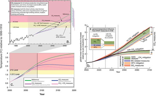
Any estimate of peak warming avoided by some future year depends critically on the assumed “reference” scenario. If one assumes that the world will adopt climate policies, then the NTCFs that are co-emitted with CO₂ will be reduced; neglecting these connections would overestimate the benefits of SLCP reductions in scenarios with explicit climate policies (Smith and Bond, 2014). For example, BC emission controls in any scenario with substantial climate-motivated CO₂ controls offer less benefit than in a no-climate policy scenario since some major BC emission sources would be phased out to reduce GHGs (Figure 12b; Rogelj et al., 2014b). Anthropogenic BC emissions in RCP8.5 are about twice as large as in RCP2.6 by 2100 (Figure S2). The magnitude of avoided warming by 2100 from CH₄ (and HFC) emission controls is lower than in a scenario without CO₂ mitigation, but smaller source overlap (Table 2) and correspondingly fewer co-benefits from CO₂ control, implies more opportunity for CH₄ (compared to BC) reductions to influence climate (Figure 12b).

Reducing SLCPs but not CO₂ can increase decadal warming rates once the SLCP emission reductions have been fully phased in (Figure 12c). Continual decreases in the rate of SLCP emissions would be needed to perpetually offset warming induced by rising CO₂, underscoring the urgency for reducing CO₂ emissions in parallel with any effort to reduce SLCPs. As for peak warming (see earlier discussion), the reference scenario choice affects the quantitative assessment of the potential for SLCPs to reduce near-term warming. Smith and Mizrahi (2013) estimate less avoided warming from SLCP reductions than Shindell et al. (2012), reflecting in part the climate-motivated CH₄ emission controls in their reference scenario. Smith and Bond (2014) find that the balance between emission controls on warming (e.g., BC) versus cooling (SO₂) NTCFs (see also Ramana et al., 2010) can either diminish or enhance, respectively, the near-term warming rates set by rising CO₂.

The GMST projections in Figure 12 rely on reduced complexity models or analytic equations that do not spatially resolve responses induced by horizontal gradients in the forcing, implicitly assuming equivalence in climate responses to any RF. Evidence exists, however, that the sensitivity of regional climate to a unit change in RF may vary by the region in which the RF occurs (Shindell and Faluvegi, 2009), and RF itself varies by region for a unit change in emissions (e.g., mid-latitudes vs. tropics; see Naik et al., 2005; W. Collins et al., 2013). In one model, different RF spatial patterns produce different regional climate responses (Shindell and Faluvegi, 2009). An analysis of four GCMs indicates that land surface temperature responses at northern mid-latitudes are sensitive to the latitude of the RF, with responses extending ~12,000 km in the zonal direction, but only ~3500 km in the meridional directions (Shindell et al., 2010). Shindell et al. (2012) apply one GCM to examine the spatial patterns of the equilibrium temperature and precipitation responses to the CH₄ versus CH₄ plus BC measures in Figure 12a, and find enhanced regional temperature responses and a shift in the Asian monsoon when BC measures are included alongside CH₄ measures. Shindell (2014) uses an ensemble of GCMs and CCMs to infer a stronger transient (i.e., near-term) response of GMST to RF from O₃ and PM due to their concentrated RF in northern mid-to-high latitudes where they can induce land responses and other amplifying feedbacks (the same mechanisms that cause GHG RF to produce amplified responses in the northern hemisphere relative to the global mean).

Rogelj et al. (2014b) compare the Shindell et al. (2012) SLCP reduction scenarios with the CLE and MFR scenarios, which explicitly consider the application of air pollution policies (Table S5). BC emissions decrease by 54% from 2010 to 2030 under CLE (implementation of planned air pollution legislation, but no explicit climate policy), as compared to the 78% reduction due to BC measures of Shindell et al. (2012), which are close to the MFR scenario (maximum pollution control but no climate policy). Under the SLCP reductions scenarios, SO₂ declines by only 2% from 2010 to 2030, yielding almost no climate disbenefit in that reference scenario. By contrast, sulfate would decrease by 45% under CLE (2010 to 2030), 72% under MFR, or 30% under climate policy (in the absence of air pollution control, to prevent atmospheric CO₂ abundances from exceeding 450 ppm). Rogelj et al. (2014b) found that stringent SO₂ emission controls lead to more near-term warming in their model than when all available BC control measures are applied. Any of these air pollution or climate policies incurs a near-term warming from SO₂ reductions, and provides grounds for an argument to reduce SLCPs to diminish the stress on human and natural systems that must adapt to this near-term warming. Near-term reductions of SCLPs might, therefore, serve as a supplement to overall climate strategies focused on CO₂ and other long-lived GHGs.

Influence of U.S. air pollutant emissions on U.S. climate

Observed ambient U.S. PM_2.5 decreased by more than 25% between 1990 and 2004 (Murphy et al., 2011), with even larger relative decreases before 1990 (Leibensperger et al., 2012b). The net RF of U.S.-sourced PM is negative, so that a reduction of PM leads to warming. Mickley et al. (2012) estimated +0.5°C warming in the eastern U.S. in a model with complete removal of U.S. anthropogenic PM. Leibensperger et al. (2012a) simulated the time course of PM cooling between 1950 and 2050, finding a maximum cooling of about 1°C in the central U.S. in concert with maximum PM in 1970–1990, following rapid declines with PM and SO₂ regulation. They attribute the observed lack of warming within the central U.S. during much of the 20th century (referred to as the “warming hole”) to U.S. PM emissions. Yu et al. (2014) also attribute the warming hole to U.S. anthropogenic PM, but invoke a different mechanism connecting PM and changes in temperature. Leibensperger et al. (2012a) also find that after SO₂ emissions peaked, U.S. warming commenced (during the 1980s and 1990s), consistent with CO₂–induced warming that is no longer masked by rising sulfate. U.S.-sourced PM likely affects climate throughout the hemisphere (Shindell and Faluvegi, 2009).

Additional changes in U.S. climate are likely as PM levels decrease (Jacobson et al., 2007; Zhang et al., 2010; Mashayekhi and Sloan, 2014). California diesel regulations have decreased ambient BC by 50% between 1998 and 2008 with an estimated lowering of local BC radiative forcing of 1.4 W m⁻² (Bahadur et al., 2012). Modeling this trend and a factor of 5 long-term BC decline in California since 1960, Ramanathan et al. (2013) find that BC reductions cooled the lower atmosphere (1–2 km) with a small warming of regional surface temperature (through the reduced absorption of solar radiation) but a net decrease in global warming.

Further decreases in PM are expected as SO₂, NO_x, and BC emissions are continuously reduced (Trail et al., 2014). The definition of “present day” must be considered when assessing the resulting climate change impacts. Many modeling studies use year 2000 as present day (e.g., Figure 4), which may not be particularly egregious on global scales as worldwide emission of SO₂, NO_x, OC, and BC may have somewhat plateaued since then. This plateau, however, reflects large U.S. and European decreases (Xing et al., 2013; Figure S1) and Asian increases (Figure S2). The U.S. contribution to global aerosol RF has fallen; a 20% decrease of year 2001 PM concentrations in North America would change global aerosol RF by +0.014 W m⁻², smaller than comparable 20% decreases in Europe and East Asia (Yu et al., 2013). Given the U.S. PM reductions realized through 2010, future reductions are unlikely to yield as large a climate change as that already observed (Leibensperger et al., 2012a). The large U.S. RF changes in Figure 4 reflect the use of 2000 as a base period. The definition of “present day” should thus be chosen with care when investigating regional climate impacts of PM (Murphy et al., 2011).

Additional challenges for air quality management

The proposed range for lowering the O₃ NAAQS level (EPA, 2014b), if adopted, might result in a relatively more important role for background O₃ in contributing to future exceedances (e.g., McDonald-Buller et al., 2011). U.S. background O₃ consists of contributions from wildfires (e.g., Emery et al., 2012; Zhang et al., 2014), stratospheric O₃ intrusions (e.g., Langford et al., 2009; 2012; M. Lin et al., 2012a), soil NO_x (e.g., Wu et al., 2008b; Hudman et al., 2010), lightning NO_x (e.g., Kaynak et al., 2008), biogenic NMVOC (e.g., Andersson and Engardt, 2010; Chen et al., 2009), and intercontinental transport (TF HTAP, 2010a), including from Asian emissions (e.g., M. Lin et al., 2012b) and global CH₄ (e.g., Clifton et al., 2014). Different model treatments of lightning NO_x, wildfires, and isoprene oxidation chemistry, as well as stratospheric intrusions contribute to discrepancies among background estimates in U.S. near-surface air, and the relative importance of a particular process varies by region and season (Fiore et al., 2014a).

Numerous studies find that reducing CH₄ emissions globally lowers the O₃ background including in near-surface air. Unlike other O₃ precursor emissions (or PM components), CH₄ RF does not depend strongly on the emission location, implying that the lowest cost CH₄ emission controls can be targeted (Fiore et al., 2002; Fiore et al., 2008). The western U.S. is particularly susceptible to pollution produced by rising Asian emissions (Jaffe et al., 1999; Jacob et al., 1999, Cooper et al., 2012), with the largest impacts in spring (Fiore et al., 2009; Reidmiller et al., 2009). Satellite products reveal trans-Pacific transport of dust (e.g., Husar et al., 2001) and CO (Heald et al., 2003), a tracer for anthropogenic pollution. A model analysis of aircraft, ground-based, and sonde data over southern California and the southwestern U.S. finds that this transported Asian pollution can be sufficiently large as to push counties above the current and proposed NAAQS levels (Lin et al., 2012b). U.S. efforts to reduce intercontinental transport or global CH₄ requires continued international discussions and agreements (e.g., TF HTAP, 2010a).

Under climate change, the western U.S. is projected to be increasingly susceptible to wildfires and the resulting PM, and possibly also to additional O₃ stratospheric intrusions (Supplementary Text S4). While these events may be classified as “exceptional events” and thus not counted against air quality determinations, a sharp uptick in frequency may render them no longer “exceptional.” In situ data needed to support exceptional event claims is often lacking, though new approaches using satellite data offer promise (e.g., Fiore et al., 2014b).

Multiple factors influence the photochemical pollution season length, such as regional meteorology, anthropogenic and biogenic emissions, and transported background. As reviewed earlier, several studies find that climate warming may extend the U.S. pollution season. Continued reductions of anthropogenic emissions lower the photochemical production of pollution in summer, but in the case of NO_x can raise O₃ levels in other seasons as titration decreases (see Supplemental Text S5). Growth in global air pollutant emissions can also lengthen the O₃ pollution season by raising the background above which regional photochemistry builds (TF HTAP, 2010a). Detecting these changes requires long-term, year-round monitoring.

Recommendations

Table 3 lists recommendations for synergistic efforts among field, laboratory, theory, and modeling approaches to fill some of the current knowledge gaps hindering a holistic approach to air quality and climate management. Projecting future climate and air quality impacts from changing emissions requires models, but their credibility is rooted in the ability to diagnose, interpret, and evaluate properly their process-level representation with high-quality measurements. While satellite data offer much promise, they too require ground-truthing, with in situ aircraft observations (e.g., Crawford and Pickering, 2014) and ground-based networks (e.g., Flynn et al., 2014; Schafer et al., 2014), particularly for PM chemical composition, which is not directly detectable from space (Hoff and Christopher, 2009). Changing land-use and agricultural practices should be examined, including their impacts on biogenic sources, which may influence air quality (e.g., Wiedinmyer et al., 2006; Heald et al., 2008; Chen et al., 2009; Jiang et al., 2010; Wu et al., 2012) and climate (Unger, 2014).

Table 3. Recommendations to fill current knowledge gaps.

Emissions

Support efforts to reduce uncertainties in the magnitude and spatial distributions in emissions inventories for air pollutants and their precursors, and their historical and recent trends Improve estimates of warming versus cooling agents emitted from individual activities and within sectors Implement, wherever possible, reporting, monitoring, and assessment programs for air pollutant and GHG emissions in undersampled regions such as developing economies and areas dominated by biogenic and other poorly quantified sources to help produce high-quality emission inventories Advance techniques to quantify emissions and their trends with higher accuracy including from satellite instruments to bound bottom-up inventories for air pollutants and GHGs Continue to analyze ice cores or other paleo records for new estimates of anthropogenic GHG and NTCF pollutant emissions since the preindustrial era to bound the impact of anthropogenic NTCFs on the climate system Update inventories rapidly to reflect the best available information from which to project future changes Consider widely varying possible future trajectories for alternative climate policy projections to the RCPs, which span only a narrow range of possibilities, to bound air quality and climate impacts from changing emissions

NTCF influence on climate

Consider two-way couplings with the stratosphere, including the role of changes in stratosphere-to-troposphere exchange on the upper tropospheric O3 burden, where it is most effective as a GHG, and of changes in CH4 on stratospheric O3, to better quantify the net impact of NTCFs on climate Observe and construct climatologies of tropospheric NTCF distributions, including vertical distributions of absorbing versus scattering PM components, NOx, and troposphere O3 to test models and bound their RF estimates Improve understanding of aerosol-cloud interactions, particularly those triggered by BC and OC including BrC, as well as sulfate, and their impacts on regional precipitation patterns Better quantify the regional effects of PM deposition on snow and ice, and the balance of regional versus long-distance transport of PM to climate-sensitive regions including the Arctic Continue to derive satellite-based RF estimates for O3 and absorbing versus scattering PM to help bound their climate impact

Effects of climate change and variability on air pollution

Assess the utility of simple global metrics and projected changes in meteorology to estimate air quality responses to regional and global climate change, and GCM skill at representing regional-scale meteorology relevant for air quality Quantify any climate penalty on air pollution incurred by changing air pollution meteorology that might confound improved air quality via precursor emission controls Use large ensemble model simulations to supplement observations and help disentangle climate change from variability Continue developing statistical approaches to characterize the frequency, spatial extent, duration, and severity of extreme pollution events Further investigate dynamical and statistical downscaling approaches to spatially refine global GCM/CCM/CTM projections, including application of model bias correction techniques Improve quantitative understanding of local-scale processes (emissions, chemistry, deposition) triggered by large-scale extreme meteorological conditions (e.g., heat waves) and their impacts on local-to-regional pollution

Cross-cutting recommendations

Advance process-level understanding of regional-scale feedbacks, including NTCF exchange with the biosphere and uncertain chemical processes (e.g., isoprene oxidation, SOA and BrC formation, tropospheric halogen chemistry, and heterogeneous chemistry) and their dependence on anthropogenic emissions Establish tools that translate research into easily digestible products that connect air pollution and climate responses to health and environmental (e.g., ecosystem, visibility) outcomes for air pollution management decisions Undertake accountability analyses of both air quality and climate impacts from past and future emission controls Improve confidence in climate sensitivity and the balance between GHG-driven warming and aerosols, including specific aerosol components, to narrow uncertainties in near- and long-term climate change Through coordinated model experiments, identify robust impacts of regional emission reductions in PM and other NTCFs relative to CO2 on temperature, precipitation, and circulation patterns relevant to pollution accumulation Examine the role of changing land-use and agricultural practices on regional climate and air pollution

Products or tools that can facilitate rapid decision making would help to inform a more holistic approach to air pollution and climate management, as information is often needed at a pace that leaves little time for existing information to be synthesized into a useful format. Concerted efforts are afoot to translate research into digestible products (e.g., Jacob et al., 2014), and to train air managers in using data products and analysis tools (Duncan et al., 2014; Streets et al., 2014; Witman et al., 2014). Published tools evaluate the benefits to climate (measured in RF) and air quality (human health impacts) under technology and policy scenarios (Akhtar et al., 2013) or from imposing fees on a single energy sector (electricity generation; Brown et al., 2013). Trade-offs will always be necessary between the statistical power of large ensembles and the complexity of process-level representation, including finer spatial resolution. Several initiatives reviewed earlier have coordinated multimodel projections (e.g., Figures 4, 8, 10), as well as quantified emission-response relationships (e.g., Wild et al., 2012), and ongoing initiatives are expected to deliver additional information on climate and air quality projections for the 21st century (Eyring and Lamarque, 2012; Eyring et al., 2013).

Conclusions

Climate and air quality are closely coupled through many processes (Figure 2). Air pollutants and their precursors are often co-emitted with CO₂ or other GHGs. Emission inventories thus underpin retrospective and future estimates of impacts from air pollutants and their precursors on climate and air quality. Many air pollutants interact with solar and terrestrial radiation, and PM components modify cloud properties, thereby altering climate through changes in temperature, precipitation, and atmospheric circulation patterns (Figures 1 and 3). Climate change alters air pollution meteorology, including large-scale stagnation events such as during heat waves, which modulate the formation and accumulation of pollution.

After CO₂, increases in CH₄ and tropospheric O₃ since the pre-industrial era have exerted the most warming of any GHGs (Figure 1), with CH₄ best documented of any NTCF. PM components exert opposing influences on the climate system. While BC alone is a strong warming agent, by some estimates even surpassing CH₄, its capacity to alter climate is subject to much larger uncertainties surrounding its interactions with clouds and to the relative fraction of BC versus co-emitted cooling OC particles that may even produce a slight net cooling from some BC-emitting sources. A portion of OC, both directly emitted and produced from gaseous organic precursors, absorbs light (BrC) and thus warms, but is not well quantified at present. Cooling sulfates have dominated the increase in anthropogenic PM during the industrial era, partially masking the warming from rising CO₂ and confounding detection of climate sensitivity from observed climate changes. Both BC and sulfate also alter precipitation patterns through interactions with clouds, in addition to circulation and other changes in response to altered local-to-global radiation budgets. The short lifetimes of PM and O₃ concentrate their abundances and climate forcing downwind of source regions, predominantly in the northern hemisphere, and thus can produce different temperature, precipitation, and circulation responses than for well-mixed GHGs with more uniform forcing distributions. An important distinction arises from the short PM and O₃ lifetimes in contrast to CO₂: the climate impacts from CO₂ depend on the cumulative CO₂ (or other long-lived GHG) emissions, while those from NTCFs depend on the emission rates.

Many source categories emit multiple GHGs and NTCFs (Figure 5). Quantifying the near- and long-term effects of reducing some or all of the emissions from such sources requires consideration of the combined effects from all of the multiple pollutants involved. Over the last 40 years, air pollution programs implemented to protect public health and welfare have decreased PM and O₃ precursors from stationary and mobile sources, particularly in developed nations, with little impact on CO₂ and CH₄ which have continued to rise. For many air pollutants, these reductions have been offset by increases in developing countries with rapidly expanding economies. An exception is SO₂ emissions, which have declined globally since the 1980s. Lowering the cooling sulfate burden “unmasks” near-term warming from GHGs (and warming particles).

Climate change is expected to degrade air quality in many polluted regions by changing air pollution meteorology (ventilation and dilution), precipitation and other removal processes and the atmospheric chemistry, anthropogenic and natural sources, which respond to changing meteorology. Modeling of alternative climate and air quality scenarios indicate a wide range in projected U.S. surface O₃ and PM_2.5. Projecting the effects of climate change on air quality can be confounded by year-to-year and decade-to-decade natural climate variability, requiring substantial computational resources to discern a climate change (signal) from the climate variability (noise). Regional climate change and the processes it triggers can offset some of the benefits from anthropogenic emission controls (the climate penalty, which includes but is not limited to emissions increases from natural and manmade sources), with some regions more sensitive than others (e.g., more wildfires in the western U.S.). Several studies find that continued regional NO_x emission reductions, such as over the eastern U.S., may guard against this climate penalty, and could lead to a full reversal of the O₃ seasonal cycle in some polluted regions. Global CH₄ increases can raise U.S. background O₃, confounding efforts to reduce U.S. O₃ via regional precursor emission controls.

Multiple linkages between air pollution and climate suggest joint mitigation might increase benefits and reduce costs, but may be challenging as the priority goals for each program can diverge. Many 21st-century projections assume that developing nations will adopt more stringent air pollution regulations for PM and O₃ to meet health and environmental goals, implying greater near-term warming rates as cooling sulfate is removed from the atmosphere. Prioritizing application of air pollutant controls on CH₄ and sources with high BC to OC ratios could offset this near-term warming induced by SO₂ emission reductions, while reducing global background O₃ and regionally high levels of PM. Lowering projected peak warming requires major CO₂ emission reductions, but has little impact on near-term climate change. Slowing the rate of increase and eventually reducing surface and tropospheric temperatures through CO₂ controls would also reduce emissions of air pollution from some source categories and minimize any climate penalty that would otherwise weaken the efficacy of future air pollution control strategies.

Acknowledgments

We are deeply grateful to John Bachmann for his numerous insights and thoughtful suggestions on multiple drafts. We acknowledge the creativity of Cathy Raphael in designing the schematic, and thank Olivia Clifton, George Milly, and Harald Rieder for generating figures. Special thanks to Patrick Dolwick and the JAWMA Critical Review Committee for constructive comments on an earlier draft, and we acknowledge useful discussions with many colleagues over the past year, including Bryan Duncan, Daniel Jacob, Loretta Mickley, Drew Shindell, and Nadine Unger. We thank several colleagues for providing their original figures.

Funding

AMF acknowledges support from the NASA Air Quality Applied Sciences Team (NNX12AF15G) and EPA STAR grant 83520601. The contents of this paper are solely the responsibility of the grantee and do not necessarily represent the official view of the EPA. Further, the EPA does not endorse the purchase of any commercial products or services mentioned in the publication.

Supplemental Materials

Supplemental data for this article can be accessed at http://dx.doi.org/10.1080/10962247.2015.1040526

Additional information

Funding

AMF acknowledges support from the NASA Air Quality Applied Sciences Team (NNX12AF15G) and EPA STAR grant 83520601. The contents of this paper are solely the responsibility of the grantee and do not necessarily represent the official view of the EPA. Further, the EPA does not endorse the purchase of any commercial products or services mentioned in the publication.

Notes on contributors

Arlene M. Fiore

Arlene M. Fiore is an associate professor in the Department of Earth and Environmental Sciences at Columbia University and Lamont-Doherty Earth Observatory. Her research areas include understanding local-to-global sources of regional air pollution, both anthropogenic and natural, as well as connections between climate, global atmospheric chemistry, and air pollution. In addition to scientific publications in these areas, she contributed to the 2006 U.S. Environmental Protection Agency (EPA) Criteria Document and the 2012 Integrated Science Assessment for the Ozone National Ambient Air Quality Standards (NAAQS), led a multi-model study on intercontinental transport of ozone under the UNECE Task Force on Hemispheric Transport of Air Pollution, and contributed to the associated reports in 2007 and 2010. Dr. Fiore was a lead author of Chapter 11 and WG1 Annex II of the Intergovernmental Panel on Climate Change Assessment Report 5 (IPCC AR5). She currently serves on the IGAC/SPARC Chemistry-Climate Modeling Initiative steering committee, is a principal investigator on the NASA Air Quality Applied Sciences Team, and a new member of the National Academy of Science’s Board on Atmospheric Sciences and Climate.

Vaishali Naik

Vaishali Naik is a scientist in the Atmospheric Chemistry & Climate Group at NOAA’s Geophysical Fluid Dynamics Laboratory. Her research centers on gaining a better understanding of the interactions between the atmospheric chemical composition and climate. She applies global chemistry-climate models and observations to assess how natural and anthropogenic activities perturb the atmospheric composition and climate. Dr. Naik is a contributing author on Chapter 11 and WG1 Annex II of the Intergovernmental Panel on Climate Change Assessment Report 5 (IPCC AR5). She also contributed to the recently conducted Atmospheric Chemistry-Climate Model Intercomparison Project (ACCMIP) that aimed to better quantify the role of short-lived pollutants in the climate system.

Eric M. Leibensperger

Eric M. Leibensperger is an assistant professor in the Center for Earth and Environmental Science at the State University of New York at Plattsburgh. Dr. Leibensperger’s research interests include atmospheric chemistry, atmospheric dynamics, and interactions between air quality and climate change. He has extensive experience using observations and modeling results to project and test the impact of climate change on air quality. He has published on the local to hemispheric air quality and climate impacts of U.S. air pollution. In addition to his research pursuits, Dr. Leibensperger is an active educator, teaching introductory and advanced courses on atmospheric science, oceanography, climate change, and scientific communication.

References

- Ackerley, D., B. B. B. Booth, S. H. E. Knight, E. J. Highwood, D. J. Frame, M. R. Allen, and D. P. Rowell. 2011. Sensitivity of twentieth-century Sahel rainfall to sulfate aerosol and CO2 forcing. J. Climate 24(19): 4999–5014. doi:10.1175/JCLI-D-11-00019.1
- Ackerman, A. S., O. B. Toon, D. E. Stevens, A. J. Heymsfield, V. Ramanathan, and E. J. Welton. 2000. Reduction of tropical cloudiness by soot. Science 288(5468): 1042–47. doi:10.1126/science.288.5468.1042
- Akhtar, F. H., R. W. Pinder, D. H. Loughlin, and D. K. Henze. 2013. GLIMPSE: A rapid decision framework for energy and environmental policy. Environ. Sci. Technol. 47(21): 12011–19. doi:10.1021/es402283j
- Albrecht, B. A. 1989. Aerosols, cloud microphysics, and fractional cloudiness. Science 245(4923): 1227–30. doi:10.1126/science.245.4923.1227
- Allen, R. J., S. C. Sherwood, J. R. Norris, and C. S. Zender. 2012. Recent Northern Hemisphere tropical expansion primarily driven by black carbon and tropospheric ozone. Nature 485(7398): 350–54. doi:10.1038/nature11097
- Alvarez, R. A., S. W. Pacala, J. J. Winebrake, W. L. Chameides, and S. P. Hamburg. 2012. Greater focus needed on methane leakage from natural gas infrastructure. Proc. Natl. Acad. Sci. USA 109(17): 6435–40. doi:10.1073/pnas.1202407109
- Amann, M., Z. Klimont, and F. Wagner. 2013. Regional and global emissions of air pollutants: Recent trends and future scenarios. Ann. Rev. Environ. Res. 38: 31–55. doi:10.1146/annurev-environ-052912-173303
- Andersson, C., and M. Engardt. 2010. European ozone in a future climate: Importance of changes in dry deposition and isoprene emissions. J. Geophys. Res. 115(D2): D02303. doi:10.1029/2008JD011690
- Andrews, T., P. M. Forster, O. Boucher, N. Bellouin, and A. Jones. 2010. Precipitation, radiative forcing and global temperature change. Geophys. Res. Lett. 37(14): L14701. doi:10.1029/2010GL043991
- Anenberg, S. C., L. W. Horowitz, D. Q. Tong, and J. J. West. 2010. An estimate of the global burden of anthropogenic ozone and fine particulate matter on premature human mortality using atmospheric modeling. Environ. Health Perspect. 118(9):1189–95. doi:10.1289/ehp.0901220
- Anenberg, S. C., J. Schwartz, D. Shindell, et al. 2012. Global air quality and health co-benefits of mitigating near-term climate change through methane and black carbon emission controls. Environ. Health. Perspect. 120(6): 831–39. doi:10.1289/ehp.1104301
- Ansari, A. S., and S. N. Pandis. 1998. Response of inorganic PM to precursor concentrations. Environ. Sci. Technol. 32(18): 2706–14. doi:10.1021/es971130j
- Appelhans, T., A. Sturman, and P. Zawar-Reza. 2012. Synoptic and climatological controls of particulate matter pollution in a Southern Hemisphere coastal city. Int. J. Climatol. 33(2): 463–79. doi:10.1002/joc.3439
- Aumont, B., R. Valorso, C. Mouchel-Vallon, M. Camredon, J. Lee-Taylor, and S. Madronich. 2012. Modeling SOA formation from the oxidation of intermediate volatility n-alkanes. Atmos. Chem. Phys. 12(16): 7577–89. doi:10.5194/acp-12-7577-2012
- Avise, J., J. Chen, B. Lamb, C. Wiedinmyer, A. Guenther, E. Salathé, and C. Mass. 2009. Attribution of projected changes in summertime US ozone and PM2.5 concentrations to global changes. Atmos. Chem. Phys. 9(4): 1111–24. doi:10.5194/acp-9-1111-2009
- Bachmann, J. 2007. Will the circle be unbroken: A history of the U.S. National Ambient Air Quality Standards. J. Air Waste Manage. 57(6): 652–97. doi:10.3155/1047-3289.57.6.652
- Bahadur, R., P. S. Praveen, Y. Xu, and V. Ramanathan. 2012. Solar absorption by elemental and brown carbon determined from spectral observations. Proc. Natl. Acad. Sci. USA 109(43): 17366–71. doi:10.1073/pnas.1205910109
- Barnes, E. A., and A. M. Fiore. 2013. Surface ozone variability and the jet position: Implications for projecting future air quality. Geophys. Res. Lett. 40(11): 2839–44. doi:10.1002/grl.50411
- Bauer, S. E., A. Bausch, L. Nazarenko, K. Tsigaridis, B. Xu, R. Edwards, M. Bisiaux, and J. McConnell. 2013. Historical and future black carbon deposition on the three ice caps: Ice core measurements and model simulations from 1850 to 2100. J. Geophys. Res. Atmos. 118(14): 7948–61. doi:10.1002/jgrd.50612
- Bauer, S. E., D. Koch, N. Unger, S. M. Metzger, D. T. Shindell, and D. G. Streets. 2007. Nitrate aerosols today and in 2030: A global simulation including aerosols and tropospheric ozone. Atmos. Chem. Phys. 7(19): 5043–59. doi:10.5194/acp-7-5043-2007
- Bellouin, N., J. Rae, A. Jones, C. Johnson, J. Haywood, and O. Boucher. 2011. Aerosol forcing in the Climate Model Intercomparison Project (CMIP5) simulations by HadGEM2-ES and the role of ammonium nitrate. J. Geophys. Res., 116: D20206. doi:10.1029/2011JD016074
- Bellouin, N., J. Quaas, J. J. Morcrette, and O. Boucher. 2013. Estimates of aerosol radiative forcing from the MACC re-analysis. Atmos. Chem. Phys. 13(4): 2045–62. doi:10.5194/acp-13-2045-2013
- Berntsen, T. K., J. S. Fuglestvedt, M. M. Joshi, K. P. Shine, N. Stuber, M. Ponater, R. Sausen, D. A. Hauglustaine, and L. Li. 2005. Response of climate to regional emissions of ozone precursors: sensitivities and warming potentials. Tellus B 57(4): 283–304. doi:10.1111/teb.2005.57.issue-4
- Biasutti, M., and A. Giannini. 2006. Robust Sahel drying in response to late 20th century forcings. Geophys. Res. Lett. 33(11): L11706. doi:10.1029/2006GL026067
- Bindoff, N. L., P. A. Stott, K. M. AchutaRao, et al. 2013. Detection and attribution of climate Change: From global to regional. In Climate Change 2013: The Physical Science Basis, Contribution of Working Group I to the Fifth Assessment Report of the Intergovernmental Panel on Climate Change, ed. T. F. Stocker, D. Qin, G.-K. Plattner, et al., 867–952. New York, NY: Cambridge University Press.
- Blanchard, C. L., S. Tanenbaum, and G. M. Hidy. 2007. Effects of sulfur dioxide and oxides of nitrogen emission reductions on fine particulate matter mass concentrations: Regional comparisons. J. Air Waste Manage. 57(11): 1337–50. doi:10.3155/1047-3289.57.11.1337
- Bloom, A. A., P. I. Palmer, A. Fraser, D. S. Reay, and C. Frankenberg. 2010. Large-scale controls of methanogenesis inferred from methane and gravity spaceborne data. Science 327(5963): 322–25. doi:10.1126/science.1175176
- Bloomer, B. J., J. W. Stehr, C. A. Piety, R. J. Salawitch, and R. R. Dickerson. 2009. Observed relationships of ozone air pollution with temperature and emissions. Geophys. Res. Lett. 36(9): L09803. doi:10.1029/2009GL037308
- Bollasina, M. A., Y. Ming, and V. Ramaswamy. 2011. Anthropogenic aerosols and the weakening of the South Asian summer monsoon. Science 334(6055): 502–5. doi:10.1126/science.1204994
- Bollasina, M. A., Y. Ming, V. Ramaswamy, M. D. Schwarzkopf, and V. Naik. 2014. Contribution of local and remote anthropogenic aerosols to the twentieth century weakening of the South Asian monsoon. Geophys. Res. Lett. 41(2): 680–87. doi:10.1002/2013GL058183
- Bond, T. C., S. J. Doherty, D. W. Fahey, et al. 2013. Bounding the role of black carbon in the climate system: A scientific assessment. J. Geophys. Res. Atmos. 118(11): 5380–52. doi:10.1002/jgrd.50171
- Boucher, O., D. Randall, P. Artaxo, et al. 2013. Clouds and aerosols. In Climate Change 2013: The Physical Science Basis, Contribution of Working Group I to the Fifth Assessment Report of the Intergovernmental Panel on Climate Change, ed. T. F. Stocker, D. Qin, G.-K. Plattner et al., 571–658. New York, NY: Cambridge University Press.
- Bowman, K., and D. K. Henze. 2012. Attribution of direct ozone radiative forcing to spatially-resolved emissions. Geophys. Res. Lett. 39: L22704. doi:10.1029/2012GL053274
- Brandt, A. R., G. A. Heath, E. A. Kort, et al. 2014. Methane leaks from North American natural gas systems. Science 343(6172): 733–35. doi:10.1126/science.1247045
- Brown, K. E., D. K. Henze, and J. B. Milford. 2013. Accounting for climate and air quality damages in future US electricity generation scenarios. Environ. Sci. Technol. 47(7): 3065–72.
- Brown-Steiner, B., P. G. Hess, and M. Y. Lin. 2015. On the capabilities and limitations of GCCM simulations of summertime regional air quality: A diagnostic analysis of ozone and temperature simulations in the US using CESM CAM-Chem. Atmos. Environ. 101: 134–48. doi:10.1016/j.atmosenv.2014.11.001
- Burnham, A., J. Han, C. E. Clark, M. Wang, J. B. Dunn, and I. Palou-Rivera. 2011. Life-cycle greenhouse gas emissions of shale gas, natural gas, coal, and petroleum. Environ. Sci. Technol. 46(2): 619–27. doi:10.1021/es201942m
- Carlton, A. G., and B. J. Turpin. 2013. Particle partitioning potential of organic compounds is highest in the eastern US and driven by anthropogenic water. Atmos. Chem. Phys. 13(20): 10203–14. doi:10.5194/acp-13-10203-2013
- Carlton, A. G., B. J. Turpin, K. E. Altieri, S. Seitzinger, A. Reff, H.-J. Lim, and B. Ervens. 2007. Atmospheric oxalic acid and SOA production from glyoxal: Results of aqueous photooxidation experiments. Atmos. Environ. 41(35): 7588–602. doi:10.1016/j.atmosenv.2007.05.035
- Carlton, A. G., B. J. Turpin, K. E. Altieri, S. P. Seitzinger, R. Mathur, S. J. Roselle, and R. J. Weber. 2008. CMAQ model performance enhanced when in-cloud secondary organic aerosol is included: Comparisons of organic carbon predictions with measurements. Environ. Sci. Technol. 42(23): 8798–802. doi:10.1021/es801192n
- Carlton, A. G., C. Wiedinmyer, and J. H. Kroll. 2009. A review of secondary organic aerosol (SOA) formation from isoprene. Atmos. Chem. Phys. 9(14): 4987–5005. doi:10.5194/acp-9-4987-2009
- Carlton, A. G., R. W. Pinder, P. V. Bhave, and G. A. Pouliot. 2010. To what extent can biogenic SOA be controlled? Environ. Sci. Technol. 44 (9):3376-–80. doi:10.1021/es903506b
- Carslaw, K. S., L. A. Lee, C. L. Reddington, K. J. Pringle, A. Rap, P. M. Forster, G. W. Mann, D. V. Spracklen, M. T. Woodhouse, L. A. Regayre, and J. R. Pierce 2013. Large contribution of natural aerosols to uncertainty in indirect forcing. Nature 503(7474): 67–71. doi:10.1038/nature12674
- Caulton, D. R., P. B. Shepson, R. L. Santoro et al. 2014. Toward a better understanding and quantification of methane emissions from shale gas development. Proc. Natl. Acad. Sci. USA 111(17): 6237–42. doi:10.1073/pnas.1316546111
- Chalmers, N., E. J. Highwood, E. Hawkins, R. Sutton, and L. J. Wilcox. 2012. Aerosol contribution to the rapid warming of near-term climate under RCP 2.6. Geophys. Res. Lett. 39(18): L18709. doi:10.1029/2012GL052848
- Chance, K., X. Liu, R. M. Suleiman, D. E. Flittner, J. Al-Saadi, and S. J. Janz. 2013. Tropospheric emissions: Monitoring of pollution (TEMPO). Proc. SPIE 8866(Earth Observing Systems XVIII). Paper 88660D.
- Chen, J., J. Avise, A. Guenther, C. Wiedinmyer, E. Salathé, R. B. Jackson, and B. Lamb. 2009. Future land use and land cover influences on regional biogenic emissions and air quality in the United States. Atmos. Environ. 43(36): 5771–80. doi:10.1016/j.atmosenv.2009.08.015
- Chen, L. W. A., J. C. Chow, X. L. Wang, J. A. Robles, B. Sumlin, D. H. Lowenthal, R. Zimmermann, and J. G. Watson. 2014. Multi-wavelength optical measurement to enhance thermal/optical analysis for carbonaceous aerosol. Atmos. Meas. Tech. Discuss. 7(9): 9173–201. doi:10.5194/amtd-7-9173-2014
- Chow, J., J. Watson, J. Robles, X. Wang, L. W. A. Chen, D. Trimble, S. Kohl, R. Tropp, and K. Fung. 2011. Quality assurance and quality control for thermal/optical analysis of aerosol samples for organic and elemental carbon. Anal. Bioanal. Chem. 401(10): 3141–52. doi:10.1007/s00216-011-5103-3
- Chow, J. C., J. G. Watson, L. W. A. Chen, G. Paredes-Miranda, M. C. O. Chang, D. Trimble, K. K. Fung, H. Zhang, and J. Zhen Yu. 2005. Refining temperature measures in thermal/optical carbon analysis. Atmos. Chem. Phys. 5(11): 2961–72. doi:10.5194/acp-5-2961-2005
- Christensen, J. H., K. Krishna Kumar, E. Aldrian, et al. 2013. Climate phenomena and their relevance for future regional climate change. In Climate Change 2013: The Physical Science Basis, Contribution of Working Group I to the Fifth Assessment Report of the Intergovernmental Panel on Climate Change, ed. T. F. Stocker, D. Qin, G.-K. Plattner, et al., 1217–308. New York, NY: Cambridge University Press.
- Chung, C. E., S. W. Kim, M. Lee, S. C. Yoon, and S. Lee. 2012. Carbonaceous aerosol AAE inferred from in-situ aerosol measurements at the Gosan ABC super site, and the implications for brown carbon aerosol. Atmos. Chem. Phys. 12(14): 6173–84. doi:10.5194/acp-12-6173-2012
- Chung, S. H., and J. H. Seinfeld. 2005. Climate response of direct radiative forcing of anthropogenic black carbon. J. Geophys. Res.-Atmos. 110(D11): D11102. doi:10.1029/2004JD005441
- Chuwah, C., T. van Noije, D. P. van Vuuren, W. Hazeleger, A. Strunk, S. Deetman, A. M. Beltran, and J. van Vliet. 2013. Implications of alternative assumptions regarding future air pollution control in scenarios similar to the representative concentration pathways. Atmos. Environ. 79: 787–801. doi:10.1016/j.atmosenv.2013.07.008
- Ciais, P., C. Sabine, G. Bala, et al. 2013. Carbon and other biogeochemical cycles. In Climate Change 2013: The Physical Science Basis, Contribution of Working Group I to the Fifth Assessment Report of the Intergovernmental Panel on Climate Change, ed. T. F. Stocker, D. Qin, G.-K. Plattner, et al., 465–570. New York, NY: Cambridge University Press.
- Clifton, O. E., A. M. Fiore, G. Correa, L. W. Horowitz, and V. Naik. 2014. Twenty-first century reversal of the surface ozone seasonal cycle over the northeastern United States. Geophys. Res. Lett. 41(20): 7343–50. doi:10.2002/2014GL061378
- Climate and Clean Air Coalition. 2014. Definitions of Short-lived Pollutants. http://www.unep.org/ccac/Short-LivedClimatePollutants/Definitions/tabid/130285/Default.aspx (accessed October 23, 2014).
- Climate Change Science Program. 2008. Climate Projections Based on Emissions Scenarios for Long-Lived And Short-Lived Radiatively Active Gases and Aerosols. Washington, DC: CCSP.
- Cofala, J., M. Amann, Z. Klimont, K. Kupiainen, and L. Höglund-Isaksson. 2007. Scenarios of global anthropogenic emissions of air pollutants and methane until 2030. Atmos. Environ. 41: 8486–99. doi:10.1016/j.atmosenv.2007.07.010
- Collins, M., R. Knutti, M. R. Allen, et al., 2013. Long-term climate change: Projections, commitments and irreversibility. In Climate Change 2013: The Physical Science Basis, Contribution of Working Group I to the Fifth Assessment Report of the Intergovernmental Panel on Climate Change, 1029–36. New York, NY: Cambridge University Press.
- Collins, W. J., M. M. Fry, H. Yu, J. S. Fuglestvedt, D. T. Shindell, and J. J. West. 2013. Global and regional temperature-change potentials for near-term climate forcers. Atmos. Chem. Phys. 13(5): 2471–85. doi:10.5194/acp-13-2471-2013
- Cook, B. I., R. L. Miller, and R. Seager. 2009. Amplification of the North American Dust Bowl drought through human-induced land degradation. P. Natl. Acad. Sci. USA 106(13): 4997–5001. doi:10.1073/pnas.0810200106
- Cooper, O. R., R.-S. Gao, D. Tarasick, T. Leblanc, and C. Sweeney. 2012. Long-term ozone trends at rural ozone monitoring sites across the United States, 1990–2010. J. Geophys. Res. Atmos. 117(D22): D22307. doi:10.1029/2012JD018261
- Cooper, O. R., J. L. Moody, D. D. Parrish, M. Trainer, T. B. Ryerson, J. S. Holloway, G. Hübler, F. C. Fehsenfeld, S. J. Oltmans, and M. J. Evans. 2001. Trace gas signatures of the airstreams within North Atlantic cyclones: Case studies from the North Atlantic Regional Experiment (NARE ’97) aircraft intensive. J. Geophys. Res. Atmos. 106(D6): 5437–456. doi:10.1029/2000JD900574
- Crawford, J. H., and K. E. Pickering 2014. DISCOVER-AQ: Advancing strategies for air quality observations in the next decade. EM, September: 4–7.
- Dawson, J. P., P. J. Adams, and S. N. Pandis. 2007a. Sensitivity of ozone to summertime climate in the eastern USA: A modeling case study. Atmos. Environ. 41(7): 1494–511. doi:10.1016/j.atmosenv.2006.10.033
- Dawson, J. P., P. J. Adams, and S. N. Pandis. 2007b. Sensitivity of PM2.5 to climate in the eastern US: A modeling case study. Atmos. Chem. Phys. 7(16): 4295–309. doi:10.5194/acp-7-4295-2007
- Dawson, J. P., B. J. Bloomer, D. A. Winner, and C. P. Weaver. 2013. Understanding the meteorological drivers of U.S. particulate matter concentrations in a changing climate. Bull. Am. Meteorol. Soc. 95(4): 521–32. doi:10.1175/BAMS-D-12-00181.1
- Day, M. C., and S. N. Pandis. 2011. Predicted changes in summertime organic aerosol concentrations due to increased temperatures. Atmos. Environ. 45(36): 6546–56. doi:10.1016/j.atmosenv.2011.08.028
- de Gouw, J. A., D. D. Parrish, G. J. Frost, and M. Trainer. 2014. Reduced emissions of CO2, NOx, and SO2 from U.S. power plants owing to switch from coal to natural gas with combined cycle technology. Earth’s Future 2(2): 75–82. doi:10.1002/eft2.2014.2.issue-2
- Dentener, F., D. Stevenson, J. Cofala, R. Mechler, M. Amann, P. Bergamaschi, F. Raes, and R. Derwent. 2005. The impact of air pollutant and methane emission controls on tropospheric ozone and radiative forcing: CTM calculations for the period 1990–2030. Atmos. Chem. Phys. 5(7): 1731–55. doi:10.5194/acp-5-1731-2005
- Dentener, F., D. Stevenson, K. Ellingsen, et al. 2006. The global atmospheric environment for the next generation. Environ. Sci. Technol. 40(11): 3586–94. doi:10.1021/es0523845
- Deser, C., R. Knutti, S. Solomon, and A. S. Phillips. 2012. Communication of the role of natural variability in future North American climate. Nature Clim. Change 2(12): 775–79. doi:10.1038/nclimate1562
- Deser, C., A. S. Phillips, M. A. Alexander, and B. V. Smoliak. 2013. Projecting North American climate over the next 50 years: Uncertainty due to internal variability. J. Climate 27(6): 2271–96. doi:10.1175/JCLI-D-13-00451.1
- Després, V. R., J. A. Huffman, S. M. Burrows, C. Hoose, A. S. Safatov, G. Buryak, J. Fröhlich-Nowoisky, W. Elbert, M. O. Andreae, U. Pöschl, and R. Jaenicke. 2012. Primary biological aerosol particles in the atmosphere: A review. Tellus B 64(2012): 1–58. doi:10.3402/tellusb.v6410.155598
- Diaz, H. F., M. P. Hoerling, and J. K. Eischeid. 2001. ENSO variability, teleconnections and climate change. Int. J. Climatol. 21(15): 1845–62. doi:10.1002/(ISSN)1097-0088
- Dlugokencky, E. J., L. Bruhwiler, J. W. C. White, et al. 2009. Observational constraints on recent increases in the atmospheric CH4 burden. Geophys. Res. Lett. 36(18): L18803. doi:10.1029/2009GL039780
- Dlugokencky, E. J., S. Houweling, L. Bruhwiler, K. A. Masarie, P. M. Lang, J. B. Miller, and P. P. Tans. 2003. Atmospheric methane levels off: Temporary pause or a new steady-state? Geophys. Res. Lett. 30(19): 1992. doi:10.1029/2003GL018126
- Dlugokencky, E. J., E. G. Nisbet, R. Fisher and D. Lowry. 2011. Global atmospheric methane: Budget, changes and dangers. Philos. Trans. R. Soc. A 369(1943): 2058–72. doi:10.1098/rsta.2010.0341
- Duncan, B. N., Y. Yoshida, B. de Foy, et al. 2013. The observed response of ozone monitoring instrument (OMI) NO2 columns to NOx emission controls on power plants in the United States: 2005–2011. Atmos. Environ. 81: 102–11. doi:10.1016/j.atmosenv.2013.08.068
- Duncan, B. N., A. I. Prados, L. N. Lamsal, et al. 2014. Satellite data of atmospheric pollution for U.S. air quality applications: Examples of applications, summary of data end-user resources, answers to FAQs, and common mistakes to avoid. Atmos. Environ. 94: 647–62. doi:10.1016/j.atmosenv.2014.05.061
- Eder, B. K., J. M. Davis, and P. Bloomfield. 1993. A characterization of the spatiotemporal variability of non-urban ozone concentrations over the eastern United States. Atmos. Environ. 27(16): 2645–68. doi:10.1016/0960-1686(93)90035-W
- Edwards, P. M., S. S. Brown, J. M. Roberts, et al. 2014. High winter ozone pollution from carbonyl photolysis in an oil and gas basin. Nature 514(7522): 351–54. doi:10.1038/nature13767
- Ehhalt, D., M. Prather, F.J. Dentener, et al. 2001. Atmospheric chemistry and greenhouse gases. In Climate Change 2001: The Physical Science Basis, Contribution of Working Group I to the Third Assessment Report of the Intergovernmental Panel on Climate Change, ed. Y. Ding, D.J. Griggs, M. Noguer, et al. New York, NY: Cambridge University Press.
- Emery, C., J. Jung, N. Downey, J. Johnson, M. Jimenez, G. Yarwood, and R. Morris. 2012. Regional and global modeling estimates of policy relevant background ozone over the United States. Atmos. Environ. 47: 206–17. doi:10.1016/j.atmosenv.2011.11.012
- Ervens, B., A. G. Carlton, B. J. Turpin, K. E. Altieri, S. M. Kreidenweis, and G. Feingold. 2008. Secondary organic aerosol yields from cloud-processing of isoprene oxidation products. Geophys. Res. Lett. 35(2): L02816. doi:10.1029/2007GL031828
- Eyring, V., and J.-F. Lamarque. 2012. Global chemistry–climate modeling and evaluation. Eos Trans. AGU 93(51): 539. doi:10.1029/2012EO510012
- Eyring, V., J.-F. Lamarque, P. Hess, et al. 2013. Overview of IGAC/SPARC Chemistry–Climate Model Initiative (CCMI) Community Simulations in Support of Upcoming Ozone and Climate Assessments. SPARC Newslett. 40: 48–66.
- Fang, Y., A. M. Fiore, L. W. Horowitz, A. Gnanadesikan, I. Held, G. Chen, G. Vecchi, and H. Levy. 2011. The impacts of changing transport and precipitation on pollutant distributions in a future climate. J. Geophys. Res. 116(D18): D18303. doi:10.1029/2011JD015642
- Fann, N., C. G. Nolte, P. Dolwick, T. L. Spero, A. C. Brown, S. Phillips, and S. Anenberg. 2015. The geographic distribution and economic value of climate change-related ozone health impacts in the United States in 2030. J. Air Waste Manag. Assoc. 65(5): 570–580. doi:10.1080/10962247.2014.996270
- Fiore, A. M., D. J. Jacob, J. A. Logan, and J. H. Yin. 1998. Long-term trends in ground level ozone over the contiguous United States, 1980–1995. J. Geophys. Res., 103: 1471–80.
- Fiore, A. M., D. J. Jacob, B. D. Field, D. G. Streets, S. D. Fernandes, and C. Jang. 2002. Linking ozone pollution and climate change: The case for controlling methane. Geophys. Res. Lett. 29(19): 1919. doi:10.1029/2002GL015601
- Fiore, A. M., J. J. West, L. W. Horowitz, V. Naik, and M. D. Schwarzkopf. 2008. Characterizing the tropospheric ozone response to methane emission controls and the benefits to climate and air quality. J. Geophys. Res. 113(D8): D08307. doi:10.1029/2007JD009162
- Fiore, A. M., F. J. Dentener, O. Wild, et al. 2009. Multimodel estimates of intercontinental source–receptor relationships for ozone pollution. J. Geophys. Res. 114(D4): D04301.
- Fiore, A. M., V. Naik, D. V. Spracklen, et al. 2012. Global air quality and climate. Chem. Soc. Rev. 41: 6663–83. doi:10.1039/c2cs35095e
- Fiore, A. M., J. T. Oberman, M. Y. Lin, L. Zhang, O. E. Clifton, D. J. Jacob, V. Naik, L. W. Horowitz, J. P. Pinto, and G. P. Milly. 2014a. Estimating North American background ozone in U.S. surface air with two independent global models: Variability, uncertainties, and recommendations. Atmos. Environ. 96(0): 284–300. doi:10.1016/j.atmosenv.2014.07.045
- Fiore, A. M., R. B. Pierce, R. R. Dickerson, and M. Y. Lin. 2014b. Detecting and attributing episodic high background ozone events. EM. February: 22–28.
- Flannigan, M. D., M. A. Krawchuk, W. J. de Groot, B. M. Wotton and L. M. Gowman. 2009. Implications of changing climate for global wildland fire. Int. J. Wildland Fire 18(5): 483–507. doi:10.1071/WF08187
- Flato, G., J. Marotzke, B. Abiodun, et al. 2013. Evaluation of climate models. In Climate Change 2013: The Physical Science Basis, Contribution of Working Group I to the Fifth Assessment Report of the Intergovernmental Panel on Climate Change, 741–866. New York, NY: Cambridge University Press.
- Flynn, C. M., K. E. Pickering, J. H. Crawford, et al. 2014. Relationship between column-density and surface mixing ratio: Statistical analysis of O3 and NO2 data from the July 2011 Maryland DISCOVER-AQ mission. Atmos. Environ. 92(0): 429–441. doi:10.1016/j.atmosenv.2014.04.041
- Ford, B., and C. L. Heald. 2013. Aerosol loading in the Southeastern United States: reconciling surface and satellite observations. Atmos. Chem. Phys. 13(18): 9269–83. doi:10.5194/acp-13-9269-2013
- Frankenberg, C., P. Bergamaschi, A. Butz, S. Houweling, J. F. Meirink, J. Notholt, A. K. Petersen, H. Schrijver, T. Warneke, and I. Aben. 2008. Tropical methane emissions: A revised view from SCIAMACHY onboard ENVISAT. Geophys. Res. Lett. 35(15): L15811. doi:10.1029/2008GL034300
- Fry, M. M., V. Naik, J. J. West, et al. 2012. The influence of ozone precursor emissions from four world regions on tropospheric composition and radiative climate forcing. J. Geophys. Res. 117(D7): D07306. doi:10.1029/2011JD017134
- Fry, M. M., M. D. Schwarzkopf, Z. Adelman, V. Naik, W. J. Collins, and J. J. West. 2013. Net radiative forcing and air quality responses to regional CO emission reductions. Atmos. Chem. Phys. 13(10): 5381–99. doi:10.5194/acp-13-5943-2013
- Fry, M. M., M. D. Schwarzkopf, Z. Adelman,and J. J. West. 2014. Air quality and radiative forcing impacts of anthropogenic volatile organic compound emissions from ten world regions. Atmos. Chem. Phys. 14(2): 523–35. doi:10.5194/acp-14-523-2014
- Fu, T.-M., D. J. Jacob, F. Wittrock, J. P. Burrows, M. Vrekoussis, and D. K. Henze. 2008. Global budgets of atmospheric glyoxal and methylglyoxal, and implications for formation of secondary organic aerosols. J. Geophys. Res. Atmos. 113(D15): D15303. doi:10.1029/2007JD009505
- Fuglestvedt, J. S., T. K. Berntsen, I. S. A. Isaksen, H. Mao, X.-Z. Liang, and W.-C. Wang. 1999. Climatic forcing of nitrogen oxides through changes in tropospheric ozone and methane; Global 3D model studies. Atmos. Environ. 33(6): 961–77. doi:10.1016/S1352-2310(98)00217-9
- Ganguly, D., P. J. Rasch, H. Wang, and J.-H. Yoon. 2012. Climate response of the South Asian monsoon system to anthropogenic aerosols. J. Geophys. Res. Atmos. 117: D13209. doi:10.1029/2012jd017508
- Gao, Y., J. S. Fu, J. B. Drake, J. F. Lamarque, and Y. Liu. 2013. The impact of emission and climate change on ozone in the United States under representative concentration pathways (RCPs). Atmos. Chem. Phys. 13: 9607–21. doi:10.5194/acp-13-9607-2013.
- Gégo, E., P. S. Porter, A. Gilliland, and S. T. Rao. 2007. Observation-based assessment of the impact of nitrogen oxides emissions reductions on ozone air quality over the eastern United States. J. Appl. Meteorol. Climatol. 46(7): 994–1008. doi:10.1175/JAM2523.1
- Geng, L., J. Cole-Dai, B. Alexander, and A. Lanciki. 2015. Recent decreases in anthropogenic aerosol load in the Arctic as observed from a Central Greenland ice core. J. Geophys. Res. in press.
- Giannini, A., M. Biasutti, I. Held, and A. Sobel. 2008. A global perspective on African climate. Climatic Change 90(4): 359–83. doi:10.1007/s10584-008-9396-y
- Ginoux, P. A., J. M. Prospero, T. E. Gill, C. Hsu, and M. Zhao. 2012. Global-scale attribution of anthropogenic and natural dust sources and their emission rates based on MODIS Deep Blue aerosol products. Rev. Geophys. 50: RG3005. doi:10.1029/2012RG000388
- Golaz, J.-C., L. W. Horowitz, and H. Levy. 2013. Cloud tuning in a coupled climate model: Impact on 20th century warming. Geophys. Res. Lett. 40(10): 2246–51. doi:10.1002/grl.50232
- Goldstein, A. H., and I. E. Galbally. 2007. Known and unexplored organic constituents in the earth’s atmosphere. Environ. Sci. Technol. 41(5): 1514–21. doi:10.1021/es072476p
- Goodrich, G. B. 2007. Influence of the Pacific decadal oscillation on winter precipitation and drought during years of neutral ENSO in the western United States. Weather Forecast. 22(1): 116–24. doi:10.1175/WAF983.1
- Gonzalez-Abraham, R., J. Avise, S. H. Chung, et al. 2014. The effects of global change upon United States air quality. Atmos. Chem. Phys. Discuss. 14: 31843–97. doi:10.5194/acpd-14-31843-2014
- Granier, C., B. Bessagnet, T. Bond, et al. 2011. Evolution of anthropogenic and biomass burning emissions of air pollutants at global and regional scales during the 1980–2010 period. Climatic Change 109: 163–90. doi:10.1007/s10584-011-0154-1
- Grythe, H., J. Ström, R. Krejci, P. Quinn, and A. Stohl. 2014. A review of sea-spray aerosol source functions using a large global set of sea salt aerosol concentration measurements. Atmos. Chem. Phys. 14(3): 1277–97. doi:10.5194/acp-14-1277-2014
- Hall, A. 2014. Projecting regional change. Science. 346: 1461–62. doi:10.1126/science.aaa0629
- Hamilton, D. S., L. A. Lee, K. J. Pringle, C. L. Reddington, D. V. Spracklen, and K. S. Carslaw 2014. Occurrence of pristine aerosol environments on a polluted planet. Proc. Natl. Acad. Sci. USA 111(52): 18466–71. doi:10.1073/pnas.1415440111
- Hansen, J., M. Sato, R. Ruedy, et al. 2005. Efficacy of climate forcings. J. Geophys. Res. 110(D18): D18104. doi:10.1029/2005JD005776
- Hauglustaine, D. A., Y. Balkanski, and M. Schulz. 2014. A global model simulation of present and future nitrate aerosols and their direct radiative forcing of climate. Atmos. Chem. Phys. Discuss. 14(5): 6863–949. doi:10.5194/acpd-14-6863-2014
- He, C., J. Liu, A. G. Carlton, S. Fan, L. W. Horowitz, H. Levy II, and S. Tao. 2013. Evaluation of factors controlling global secondary organic aerosol production from cloud processes. Atmos. Chem. Phys. 13(4): 1913–26. doi:10.5194/acp-13-1913-2013
- Heald, C. L., D. J. Jacob, A. M. Fiore, et al. 2003. Asian outflow and trans-Pacific transport of carbon monoxide and ozone pollution: An integrated satellite, aircraft, and model perspective. J. Geophys. Res. 108(D24): 4804. doi:10.1029/2003JD003507
- Heald, C. L., D. K. Henze, L. W. Horowitz, et al. 2008. Predicted change in global secondary organic aerosol concentrations in response to future climate, emissions, and land use change. J. Geophys. Res. 113(D5): D05211. doi:10.1029/2007JD009092
- Heald, C. L., D. J. Jacob, R. J. Park, L. M. Russell, B. J. Huebert, J. H. Seinfeld, H. Liao, and R. J. Weber. 2005. A large organic aerosol source in the free troposphere missing from current models. Geophys. Res. Lett. 32(18): L18809. doi:10.1029/2005GL023831
- Heald, C. L., D. A. Ridley, J. H. Kroll, S. R. H. Barrett, K. E. Cady-Pereira, M. J. Alvarado, and C. D. Holmes. 2014. Contrasting the direct radiative effect and direct radiative forcing of aerosols. Atmos. Chem. Phys. 14(11): 5513–27. doi:10.5194/acp-14-5513-2014
- Hedegaard, G. B., J. H. Christensen, and J. Brandt. 2013. The relative importance of impacts from climate change vs. emissions change on air pollution levels in the 21st century. Atmos. Chem. Phys. 13: 3569–85. doi:10.5194/acp-13-3569-2013
- Hegarty, J., H. Mao, and R. Talbot. 2007. Synoptic controls on summertime surface ozone in the northeastern United States. J. Geophys. Res. Atmos. 112(D14): D14306. doi:10.1029/2006JD008170
- Held, I. M., M. Winton, K. Takahashi, T. Delworth, F. Zeng, and G. K. Vallis. 2010. Probing the fast and slow components of global warming by returning abruptly to preindustrial forcing. J. Climate. 23(9): 2418–27. doi:10.1175/2009JCLI3466.1
- Henze, D. K., D. T. Shindell, F. Akhtar, R. J. D. Spurr, R. W. Pinder, D. Loughlin, M. Kopacz, K. Sing,h and C. Shim. 2012. Spatially refined aerosol direct radiative forcing efficiencies. Environ. Sci. Technol. 46(17): 9511–18. doi:10.1021/es301993s
- Hessl, A. E., D. McKenzie, and R. Schellhaas. 2004. Drought and Pacific decadal oscillation linked to fire occurrence in the inland Pacific Northwest. Ecol. Appl. 14(2): 425–42. doi:10.1890/03-5019
- Hidy, G. M., and W. T. Pennell. 2010. Multipollutant air quality management. J. Air Waste Manag. Assoc. 60(6): 645–74. doi:10.3155/1047-3289.60.6.645
- Hoff, R. M., and S. A. Christopher. 2009. Remote sensing of particulate pollution from space: Have we reached the promised land? J. Air Waste Manag. Assoc. 59: 645–75. doi:10.3155/1047-3289.59.6.645
- Holmes, C. D., M. J. Prather, O. A. Søvde, and G. Myhre. 2013. Future methane, hydroxyl, and their uncertainties: key climate and emission parameters for future predictions. Atmos. Chem. Phys. 13(1): 285–302. doi:10.5194/acp-13-285-2013
- Holmes, C. D., Q. Tang, and M. J. Prather. 2011. Uncertainties in climate assessment for the case of aviation NO. Proc. Natl. Acad. Sci. USA. 108(27): 10997–1002. doi:10.1073/pnas.1101458108
- Horton, D. E., Harshvardhan, and N. S. Diffenbaugh. 2012. Response of air stagnation frequency to anthropogenically enhanced radiative forcing. Environ. Res. Lett. 7(4): 044034. doi:10.1088/1748-9326/7/4/044034
- Horton, D. E., C. B. Skinner, D. Singh, and N. S. Diffenbaugh. 2014. Occurrence and persistence of future atmospheric stagnation events. Nature Clim. Change. 4(8): 698–703. doi:10.1038/nclimate2272
- Hoyle, C. R., M. Boy, N. M. Donahue, et al. 2011. A review of the anthropogenic influence on biogenic secondary organic aerosol. Atmos. Chem. Phys. 11(1): 321–43. doi:10.5194/acp-11-321-2011
- Hudman, R. C., A. R. Russell, L. C. Valin, and R. C. Cohen. 2010. Interannual variability in soil nitric oxide emissions over the United States as viewed from space. Atmos. Chem. Phys. 10(20): 9943–52. doi:10.5194/acp-10-9943-2010
- Huneeus, N. M., M. Schulz, Y. Balkanski, et al. 2011. Global dust model intercomparison in AeroCom phase I. Atmos. Chem. Phys. 11(15): 7781–816. doi:10.5194/acp-11-7781-2011
- Husain, L., A. J. Kahn, T. Ahmed, K. Swami, A. Bari, J. S. Webber, and J. Li. 2008. Trends in atmospheric elemental carbon concentrations from 1835 to 2005. J. Geophys. Res. 113: D13102. doi:10.1029/2007JD009398
- Husar, R. B., et al. 2001. Asian dust events of April 1998. J. Geophys. Res. 106(D16): 18317–30. doi:10.1029/2000JD900788
- Hwang, Y.-T., D. M. W. Frierson, and S. M. Kang. 2013. Anthropogenic sulfate aerosol and the southward shift of tropical precipitation in the late 20th century. Geophys. Res. Lett. 40(11): 2845–50. doi:10.1002/grl.50502
- Igel, A. L., S. C. van den Heever, C. M. Naud, S. M. Saleeby, and D. J. Posselt. 2013. Sensitivity of Warm-Frontal Processes to Cloud-Nucleating Aerosol Concentrations. J. Atmos. Sci. 70(6): 1768–83. doi:10.1175/JAS-D-12-0170.1
- Intergovernmental Panel on Climate Change. 2013a. Climate Change 2013: The Physical Science Basis, Contribution of Working Group I to the Fifth Assessment Report of the Intergovernmental Panel on Climate Change. New York, NY: Cambridge University Press.
- Intergovernmental Panel on Climate Change. 2013b. Annex II: Climate system scenario tables. In Climate Change 2013: The Physical Science Basis, Contribution of Working Group I to the Fifth Assessment Report of the Intergovernmental Panel on Climate Change, ed. T. F. Stocker, D. Qin, G.-K. Plattner, et al., 1395–446. New York, NY: Cambridge University Press.
- Intergovernmental Panel on Climate Change. 2013c. Summary for policymakers. In Climate Change 2013: The Physical Science Basis, Contribution of Working Group I to the Fifth Assessment Report of the Intergovernmental Panel on Climate Change, ed. T. F. Stocker, D. Qin, G.-K. Plattner, et al., 1–30. New York, NY: Cambridge University Press.
- Intergovernmental Panel on Climate Change. 2013d. Annex III: Glossary. In Climate Change 2013: The Physical Science Basis, Contribution of Working Group I to the Fifth Assessment Report of the Intergovernmental Panel on Climate Change, ed. T. F. Stocker, D. Qin, G.-K. Plattner, et al., 1447–66. New York, NY: Cambridge University Press.
- Intergovernmental Panel on Climate Change. 2014. Climate Change 2014: Synthesis Report, Contribution of Working Groups I, II and III to the Fifth Assessment Report of the Intergovernmental Panel on Climate Change [Core writing team, R. K. Pachauri and L. A. Meyer, eds.]. Geneva, Switzerland: IPCC.
- Isaksen, I. S. A., C. Granier, G. Myhre, et al. 2009. Atmospheric composition change: Climate–chemistry interactions, Atmos. Environ. 43: 5138–92. doi:10.1016/j.atmosenv.2009.08.003
- Jacob, D. J., T. Holloway, and J. D. Haynes. 2014. The NASA Air Quality Applied Sciences Team (AQAST). EM February: 4–5.
- Jacob, D. J., J. A. Logan, and P. P. Murti. 1999. Effect of rising Asian emissions on surface ozone in the United States. Geophys. Res. Lett. 26(14): 2175–78. doi:10.1029/1999GL900450
- Jacob, D. J., and D. A. Winner. 2009. Effect of climate change on air quality. Atmos. Environ. 43(1): 51–63. doi:10.1016/j.atmosenv.2008.09.051
- Jacobson, M. Z. 2000. A physically-based treatment of elemental carbon optics: Implications for global direct forcing of aerosols. Geophys. Res. Lett. 27(2): 217–20. doi:10.1029/1999GL010968
- Jacobson, M. Z. 2007. Effects of ethanol (E85) versus gasoline vehicles on cancer and mortality in the United States. Environ. Sci. Technol. 41(11): 4150–57. doi:10.1021/es062085v
- Jacobson, M. Z. 2010. Short-term effects of controlling fossil-fuel soot, biofuel soot and gases, and methane on climate, Arctic ice, and air pollution health. J. Geophys. Res. Atmos. 115(D14): D14209. doi:10.1029/2009JD013795
- Jacobson, M. Z. 2012. Investigating cloud absorption effects: Global absorption properties of black carbon, tar balls, and soil dust in clouds and aerosols. J. Geophys. Res. Atmos. 117(D6): D06205. doi:10.1029/2011JD017218
- Jacobson, M. Z. 2014. Effects of biomass burning on climate, accounting for heat and moisture fluxes, black and brown carbon, and cloud absorption effects. J. Geophys. Res. Atmos. 119(14): 2014JD021861. doi:10.1002/2014JD021861
- Jacobson, M., Y. Kaufman, and Y. Rudich. 2007. Examining feedbacks of aerosols to urban climate with a model that treats 3-D clouds with aerosol inclusions. J. Geophys. Res. Atmos. 112: D24205. doi:10.1029/2007JD008922
- Jaeglé, L., P. K. Quinn, T. S. Bates, B. Alexander, and J. T. Lin. 2011. Global distribution of sea salt aerosols: new constraints from in situ and remote sensing observations. Atmos. Chem. Phys. 11(7): 3137–57. doi:10.5194/acp-11-3137-2011
- Jaffe, D., T. Anderson, D. Covert, et al. 1999. Transport of Asian air pollution to North America. Geophys. Res. Lett. 26(6): 711–14. doi:10.1029/1999GL900100
- Jiang, X., Z.-L. Yang, H. Liao, and C. Wiedinmyer. 2010. Sensitivity of biogenic secondary organic aerosols to future climate change at regional scales: An online coupled simulation. Atmos. Environ. 44(38): 4891–907. doi:10.1016/j.atmosenv.2010.08.032
- John, J. G., A. M. Fiore, V. Naik, L. W. Horowitz, and J. P. Dunne. 2012. Climate versus emission drivers of methane lifetime against loss by tropospheric OH from 1860–2100. Atmos. Chem. Phys. 12(24): 12021–36. doi:10.5194/acp-12-12021-2012
- Jones, A., J. M. Haywood, and O. Boucher. 2007. Aerosol forcing, climate response and climate sensitivity in the Hadley Centre climate model. J. Geophys. Res. Atmos. 112(D20): D20211. doi:10.1029/2007JD008688
- Kalina, E. A., K. Friedrich, H. Morrison, and G. H. Bryan. 2014. Aerosol effects on idealized supercell thunderstorms in different environments. J. Atmos. Sci. 71(12): 4558–80. doi:10.1175/JAS-D-14-0037.1
- Karion, A., C. Sweeney, G. Pétron, et al. 2013. Methane emissions estimate from airborne measurements over a western United States natural gas field. Geophys. Res. Lett. 40(16): 4393–97. doi:10.1002/grl.50811
- Kaynak, B., Y. Hu, R. V. Martin, A. G. Russell, Y. Choi, and Y. Wang. 2008. The effect of lightning NOx production on surface ozone in the continental United States. Atmos. Chem. Phys. 8(17): 5151–59. doi:10.5194/acp-8-5151-2008
- Keene, W. C., J. L. Moody, J. N. Galloway, J. M. Prospero, O. R. Cooper, S. Eckhardt, and J. R. Maben. 2014. Long-term trends in aerosol and precipitation composition over the western North Atlantic Ocean at Bermuda. Atmos. Chem. Phys. 14(15): 8119–35. doi:10.5194/acp-14-8119-2014
- Kelly, J., P. A. Makar, and D. A. Plummer. 2012. Projections of mid-century summer air-quality for North America: effects of changes in climate and precursor emissions. Atmos. Chem. Phys. 12: 5367–90. doi:10.5194/acp-12-5367-2012
- Kiehl, J. T. 2007. Twentieth century climate model response and climate sensitivity. Geophys. Res. Lett. 34(22): L22710. doi:10.1029/2007GL031383
- Kirschke, S., P. Bousquet, P. Ciais, et al. 2013. Three decades of global methane sources and sinks. Nat. Geosci. 6: 813–23. doi:10.1038/ngeo1955
- Kirtman, B., S.B. Power, J.A. Adedoyin, et al., 2013. Near-term climate change: Projections and predictability. In Climate Change 2013: The Physical Science Basis, Contribution of Working Group I to the Fifth Assessment Report of the Intergovernmental Panel on Climate Change, 953–1028. New York, NY: Cambridge University Press.
- Kleeman, M. J. 2008. A preliminary assessment of the sensitivity of air quality in California to global change. Climatic Change 87 (Suppl. 1): S273–92. doi:10.1007/s10584-007-9351-3
- Klimont, Z., S. J. Smith, and J. Cofala. 2013. The last decade of global anthropogenic sulfur dioxide: 2000–2011 Emissions. Environ. Res. Lett. 8:014003. doi:10.1088/1748-9326/8/1/014003
- Klingmüller, K., B. Steil, C. Brühl, H. Tost, and J. Lelieveld. 2014. Sensitivity of aerosol radiative effects to different mixing assumptions in the AEROPT 1.0 submodel of the EMAC atmospheric-chemistry–climate model. Geosci. Model Dev. 7(5): 2503–16. doi:10.5194/gmd-7-2503-2014
- Kloster, S., F. Dentener, J. Feichter, et al. 2008. Influence of future air pollution mitigation strategies on total aerosol radiative forcing. Atmos. Chem. Phys. 8: 6405–37. doi:10.5194/acp-8-6405-2008
- Kloster, S., F. Dentener, J. Feichter, F. Raes, U. Lohmann, E. Roeckner, and I. Fischer-Bruns. 2009. A GCM study of future climate response to aerosol pollution reductions. Clim. Dyn. 34(7): 1177–94. doi:10.1007/s00382-009-0573-0
- Knutti, R. 2008. Why are climate models reproducing the observed global surface warming so well? Geophys. Res. Lett. 35(18): L18704. doi:10.1029/2008GL034932
- Koch, D., M. Schulz, S. Kinne, et al. 2009a. Evaluation of black carbon estimations in global aerosol models. Atmos. Chem. Phys. 9(22): 9001–26. doi:10.5194/acp-9-9001-2009
- Koch, D., S. Menon, A. Del Genio, R. Ruedy, I. Alienov, and G. A. Schmidt. 2009b. Distinguishing aerosol impacts on climate over the past century. J. Climate 22(10): 2659–77. doi:10.1175/2008JCLI2573.1
- Köhler, M. O., G. Rädel, K. P. Shine, H. L. Rogers, and J. A. Pyle. 2013. Latitudinal variation of the effect of aviation NOx emissions on atmospheric ozone and methane and related climate metrics. Atmos. Environ. 64(0): 1–9. doi:10.1016/j.atmosenv.2012.09.013
- Kort, E. A., C. Frankenberg, K. R. Costigan, R. Lindenmaier, M. K. Dubey, and D. Wunch. 2014. Four corners: The largest US methane anomaly viewed from space. Geophys. Res. Lett. 41 (19): 2014GL061503. doi:10.1002/2014GL061503
- Koumoutsaris, S., I. Bey, S. Generoso, and V. Thouret. 2008. Influence of El Nino–Southern Oscillation on the interannual variability of tropospheric ozone in the northern midlatitudes. J. Geophys. Res. 113(D19): D19301. doi:10.1029/2007JD009753
- Kurokawa, J., T. Ohara, T. Morikawa, et al. 2013. Emissions of air pollutants and greenhouse gases over Asian regions during 2000–2008: Regional Emission inventory in ASia (REAS) version 2. Atmos. Chem. Phys. 13: 11019–58. doi:10.5194/acp-13-11019-2013
- Lam, N. L., et al. 2012. Household light makes global heat: high black carbon emissions from kerosene wick lamps. Environ. Sci. Technol. 46(24): 13531–38. doi:10.1021/es302697h
- Lamarque, J. F., et al. 2010. Historical (1850–2000) gridded anthropogenic and biomass burning emissions of reactive gases and aerosols: methodology and application. Atmos. Chem. Phys. 10: 7017–39. doi:10.5194/acp-10-7017-2010
- Lamarque, J. F., D. T. Shindell, B. Josse, et al. 2013. The Atmospheric Chemistry and Climate Model Intercomparison Project (ACCMIP): overview and description of models, simulations and climate diagnostics. Geosci. Model Dev. 6: 179–206. doi:10.5194/gmd-6-179-2013
- Lambe, A. T., C. D. Cappa, P. Massoli, et al. 2013. Relationship between oxidation level and optical properties of secondary organic aerosol. Environ. Sci. Technol. 47(12): 6349–57. doi:10.1021/es401043j
- Lamsal, L. N., B. N. Duncan, Y. Yoshida, K. Nickolay, K. E. Pickering, D. G. Streets, and L. Zifeng. 2015. EPA Air Quality System (AQS) data versus improved observations from the ozone monitoring instrument (OMI). Atmos. Environ. 110(0): 130–43. doi:10.1016/j.atmosenv.2015.03.055
- Langford, A. O., T. J. O’Leary, C. D. Masters, K. C. Aikin, and M. H. Proffitt. 1998. Modulation of middle and upper tropospheric ozone at northern midlatitudes by the El Niño/Southern Oscillation. Geophys. Res. Lett. 25(14): 2667–70. doi:10.1029/98GL01909
- Langford, A. O., K. C. Aikin, C. S. Eubank, and E. J. Williams. 2009. Stratospheric contribution to high surface ozone in Colorado during springtime. Geophys. Res. Lett. 36: L12801. doi:10.1029/2009GL038367
- Langford, A. O., J. Brioude, O. R. Cooper, C. J. Senff, R. J. Alvarez II, R. M. Hardesty, B. J. Johnson, and S. J. Oltmans. 2012. Stratospheric influence on surface ozone in the Los Angeles area during late spring and early summer of 2010. J. Geophys. Res. 117:D00V06. doi:10.1029/2011JD016766
- Lee, Y.H., et al. 2013. Evaluation of preindustrial to present-day black carbon and its albedo forcing from Atmospheric Chemistry and Climate Model Intercomparison Project (ACCMIP). Atmos. Chem. Phys. 13: 2607–34. doi:10.5194/acp-13-2607-2013
- Lehmann, C. B., V. Bowersox, R. Larson, and S. Larson. 2007. Monitoring long-term trends in sulfate and ammonium in US precipitation: Results from the National Atmospheric Deposition Program/National Trends Network. In Acid Rain—Deposition to Recovery, ed. P. Brimblecombe, H. Hara, D. Houle, and M. Novak, 59–66. Dordrecht, The Netherlands: Springer.
- Lei, H., D. J. Wuebbles, and X.-Z. Liang. 2012. Projected risk of high ozone episodes in 2050. Atmos. Environ. 59: 567–77. doi:10.1016/j.atmosenv.2012.05.051
- Leibensperger, E. M., L. J. Mickley, and D. J. Jacob. 2008. Sensitivity of US air quality to mid-latitude cyclone frequency and implications of 1980–2006 climate change. Atmos. Chem. Phys. 8(23): 7075–86. doi:10.5194/acp-8-7075-2008
- Leibensperger, E. M., L. J. Mickley, D. J. Jacob, and S. R. H. Barrett. 2011. Intercontinental influence of NOx and CO emissions on particulate matter air quality. Atmos. Environ. 45(19): 3318–24. doi:10.1016/j.atmosenv.2011.02.023
- Leibensperger, E. M., L. J. Mickley, D. J. Jacob, W. T. Chen, J. H. Seinfeld, A. Nenes, P. J. Adams, D. G. Streets, N. Kumar, and D. Rind. 2012a. Climatic effects of 1950–2050 changes in US anthropogenic aerosols—Part 2: Climate response. Atmos. Chem. Phys. 12(7): 3349–62.
- Leibensperger, E. M., L. J. Mickley, D. J. Jacob, W. T. Chen, J. H. Seinfeld, A. Nenes, P. J. Adams, D. G. Streets, N. Kumar, and D. Rind. 2012b. Climatic effects of 1950–2050 changes in US anthropogenic aerosols—Part 1: Aerosol trends and radiative forcing. Atmos. Chem. Phys. 12(7): 3333–48. doi:10.5194/acp-12-3333-2012
- Levy, H.II, M. D. Schwarzkopf, L. Horowitz, V. Ramaswamy, and K. L. Findell. 2008. Strong sensitivity of late 21st century climate to projected changes in short-lived air pollutants. J. Geophys. Res. 113: D06102. doi:10.1029/2007JD009176
- Levy, H.II, L. W. Horowitz, M. D. Schwarzkopf, Y. Ming, J.-C. Golaz, V. Naik, and V. Ramaswamy. 2013. The roles of aerosol direct and indirect effects in past and future climate change. J. Geophys. Res. Atmos. 118: 4521–32. doi:10.1002/jgrd.50192
- Li, J., W.-C. Wang, H. Liao, and W. Chang. 2014. Past and future direct radiative forcing of nitrate aerosol in East Asia. Theor. Appl. Climatol. 1–14. doi:10.1007/s00704-014-1249-1
- Liao, H., and J. H. Seinfeld. 2005. Global impacts of gas-phase chemistry-aerosol interactions on direct radiative forcing by anthropogenic aerosols and ozone. J. Geophys. Res. Atmos. 110(D18): D18208. doi:10.1029/2005JD005907
- Lim, H.-J., A. G. Carlton, and B. J. Turpin. 2005. Isoprene forms secondary organic aerosol through cloud processing: Model simulations. Environ. Sci. Technol. 39(12): 4441–46. doi:10.1021/es048039h
- Lin, C. Y. C., D. J. Jacob,and A. M. Fiore. 2001. Trends in exceedances of the ozone air quality standard in the continental United States, 1980–1998. Atmos. Environ. 35(19): 3217–228. doi:10.1016/S1352-2310(01)00152-2
- Lin, G., S. Sillman, J. E. Penner, and A. Ito. 2014. Global modeling of SOA: The use of different mechanisms for aqueous-phase formation. Atmos. Chem. Phys. 14: 5451–75. doi:10.5194/acp-14-5451-2014
- Lin, M., A. M. Fiore, O. R. Cooper, L. W. Horowitz, A. O. Langford, H. Levy, B. J. Johnson, V. Naik, S. J. Oltmans, and C. J. Senff. 2012a. Springtime high surface ozone events over the western United States: Quantifying the role of stratospheric intrusions. J. Geophys. Res. Atmos. 117(D21): D00V22. doi:10.1029/2012JD018151
- Lin, M., A. M. Fiore, L. W. Horowitz, et al. 2012b. Transport of Asian ozone pollution into surface air over the western United States in spring. J. Geophys. Res. 117: D00V07. doi:10.1029/2011JD016961
- Lin, M., L. W. Horowitz, S. J. Oltmans, A. M. Fiore, and S. Fan. 2014. Tropospheric ozone trends at Mauna Loa Observatory tied to decadal climate variability. Nat. Geosci. 7(2): 136–43. doi:10.1038/ngeo2066
- Litovitz, A., A. Curtright, S. Abramzon, N. Burger, and C. Samaras. 2013. Estimation of regional air-quality damages from Marcellus Shale natural gas extraction in Pennsylvania. Environ. Res. Lett. 8:014017. doi:10.1088/1748-9326/8/1/014017
- Logan, J. A. 1989. Ozone in rural areas of the United States. J. Geophys. Res. 94(D6): 8511–32. doi:10.1029/JD094iD06p08511
- Mahowald, N. 2011. Aerosol indirect effect on biogeochemical cycles and climate. Science 334(6057): 794–96. doi:10.1126/science.1207374
- Makkonen, R., A. Asmi, V. M. Kerminen, M. Boy, A. Arneth, P. Hari, and M. Kulmala. 2012. Air pollution control and decreasing new particle formation lead to strong climate warming. Atmos. Chem. Phys. 12(3): 1515–24. doi:10.5194/acp-12-1515-2012
- Mansell, E. R., and C. L. Ziegler. 2013. Aerosol effects on simulated storm electrification and precipitation in a two-moment bulk microphysics model. J. Atmos. Sci. 70(7): 2032–50. doi:10.1175/JAS-D-12-0264.1
- Mashayekhi, R., and J. J. Sloan. 2014. Effects of aerosols on precipitation in north-eastern North America. Atmos. Chem. Phys. 14(10): 5111–25. doi:10.5194/acp-14-5111-2014
- Masui, T., K. Matsumoto, Y. Hijioka, et al. 2011. An emission pathway for stabilization at 6 Wm−2 radiative forcing. Climatic Change 109: 59–76. doi:10.1007/s10584-011-0150-5
- Matthews, E. 2012. Good News From the Dump. Paper for the Clean Air Task Force, Boston, MA.
- McConnell, J. R., A. J. Aristarain, J. R. Banta, P. R. Edwards, and J. C. Simoes. 2007a. 20th-Century doubling in dust archived in an Antarctic Peninsula ice core parallels climate change and desertification in South America. Proc. Natl. Acad. Sci. USA 104(14): 5743–48. doi:10.1073/pnas.0607657104
- McConnell, J. R., R. Edwards, G. L. Kok, M. G. Flanner, C. S. Zender, E. S. Saltzman, J. R. Banta, D. R. Pasteris, M. M. Carter, and J. D. W. Kahl. 2007b. 20th Century industrial black carbon emissions altered Arctic climate forcing. Science 317(5843): 1381–84. doi:10.1126/science.1144856
- McDonald-Buller, E. C., D. T. Allen, N. Brown, et al. 2011. Establishing policy relevant background (PRB) ozone concentrations in the United States. Environ. Sci. Technol. 45(22): 9484–97. doi:10.1021/es2022818
- McNeill, V. F. 2015. Aqueous organic chemistry in the atmosphere: Sources and chemical processing of organic aerosols. Environ. Sci. Technol. 49(3): 1237–44. doi:10.1021/es5043707
- McNeill, V. F., J. L. Woo, D. D. Kim, A. N. Schwier, N. J. Wannell, A. J. Sumner, and J. M. Barakat. 2012. Aqueous-phase secondary organic aerosol and organosulfate formation in atmospheric aerosols: A modeling study. Environ. Sci. Technol. 46(15): 8075–81. doi:10.1021/es3002986
- Mearns, L. O., W. J. Gutowski, R. Jones, L.-Y. Leung, S. McGinnis, A. M. B. Nunes, and Y. Qian. 2009. A regional climate change assessment program for North America. EOS 90(36) 8: 311–12. doi:10.1029/2009EO360002
- Mearns, L. O., et al. 2012. The North American Regional Climate Change Assessment Program: Overview of phase I results. Bull. Am. Meteor. Soc. 93: 1337–62. doi:10.1175/BAMS-D-11-00223.1
- Meehl, G. A., T. F. Stocker, W. D. Collins, et al. 2007. Global climate projections. In Climate Change 2007: The Physical Science Basis, Contribution of Working Group I to the Fourth Assessment Report of the Intergovernmental Panel on Climate Change, ed. S. Solomon, D. Qin M. Manning, Z. Chen, et al., 747–845, New York, NY: Cambridge University Press.
- Meehl, G. A., J. M. Arblaster, and W. D. Collins. 2008. Effects of black carbon aerosols on the Indian monsoon. J. Climate. 21(12): 2869–82. doi:10.1175/2007JCLI1777.1
- Meinshausen, M., S. J. Smith, K. Calvin, et al. 2011. The RCP greenhouse gas concentrations and their extensions from 1765 to 2300. Climatic Change 109: 213–41. doi:10.1007/s10584-011-0156-z
- Melillo, J. M., T. C. Richmond, and G. W. Yohe. 2014. Climate Change Impacts in the United States: The Third National Climate Assessment, 841. U.S. Global Change Research Program, Washington, DC.
- Menon, S., J. Hansen, L. Nazarenko, and Y. Luo. 2002. Climate effects of black carbon aerosols in China and India. Science 297(5590): 2250–53. doi:10.1126/science.1075159
- Merlis, T. M., M. Zhao and I. M. Held. 2013. The sensitivity of hurricane frequency to ITCZ changes and radiatively forced warming in aquaplanet simulations. Geophys. Res. Lett. 40(15): 4109–14. doi:10.1002/grl.50680
- Mickley, L. J., D. J. Jacob, B. D. Field, and D. Rind. 2004. Effects of future climate change on regional air pollution episodes in the United States. Geophys. Res. Lett. 30: L24103. doi:10.1029/2004GL021216
- Mickley, L. J., E. M. Leibensperger, D. J. Jacob, and D. Rind. 2012. Regional warming from aerosol removal over the United States: Results from a transient 2010–2050 climate simulation. Atmos. Environ. 46(0): 545–53. doi:10.1016/j.atmosenv.2011.07.030
- Mikaloff Fletcher, S. E., P. P. Tans, L. M. Bruhwiler, J. B. Miller, and M. Heimann. 2004a. CH4 sources estimated from atmospheric observations of CH4 and its 13C/12C isotopic ratios: 1. Inverse modeling of source processes. Global Biogeochem. Cycles 18 (4): GB4004. doi:10.1029/2004GB002223
- Mikaloff Fletcher, S. E., P. P. Tans, L. M. Bruhwiler, J. B. Miller, and M. Heimann. 2004b. CH4 sources estimated from atmospheric observations of CH4 and its 13C/12C isotopic ratios: 2. Inverse modeling of CH4 fluxes from geographical regions. Global Biogeochem. Cycles 18 (4): GB4005. doi:10.1029/2004GB002224
- Miller, S. M., et al. 2013. Anthropogenic emissions of methane in the United States. Proc. Natl. Acad. Sci. USA 110(50): 20018–22. doi:10.1073/pnas.1314392110
- Ming, Y., V. Ramaswamy, and G. Chen. 2011. A model investigation of aerosol-induced changes in boreal winter extratropical circulation. J. Climate 24(23): 6077–91. doi:10.1175/2011JCLI4111.1
- Ming, Y., V. Ramaswamy, and G. Persad. 2010. Two opposing effects of absorbing aerosols on global-mean precipitation. Geophys. Res. Lett. 37(13): L13701. doi:10.1029/2010GL042895
- Monteil, G., S. Houweling, E. J. Dlugockenky, G. Maenhout, B. H. Vaughn, J. W. C. White, and T. Rockmann. 2011. Interpreting methane variations in the past two decades using measurements of CH4 mixing ratio and isotopic composition. Atmos. Chem. Phys. 11: 9141–53. doi:10.5194/acp-11-9141-2011
- Morrison, H. 2012. On the robustness of aerosol effects on an idealized supercell storm simulated with a cloud system-resolving model. Atmos. Chem. Phys. 12(16): 7689–705. doi:10.5194/acp-12-7689-2012
- Moss, R. H., J. A. Edmonds, K. A. Hibbard, et al. 2010. The next generation of scenarios for climate change research and assessment. Nature 463: 747–56. doi:10.1038/nature08823
- Murphy, D. M., J. C. Chow, E. M. Leibensperger, W. C. Malm, M. Pitchford, B. A. Schichtel, J. G. Watson, and W. H. White. 2011. Decreases in elemental carbon and fine particle mass in the United States. Atmos. Chem. Phys. 11(10): 4679–86. doi:10.5194/acp-11-4679-2011
- Myhre, G. 2009. Consistency between satellite-derived and modeled estimates of the direct aerosol effect. Science 325(5937): 187–90. doi:10.1126/science.1174461
- Myhre, G., D. Shindell, F.-M. Breon, et al. 2013a. Anthropogenic and natural radiative forcing. In Climate Change 2013: The Physical Science Basis, Contribution of Working Group I to the Fifth Assessment Report of the Intergovernmental Panel on Climate Change, ed. T. F. Stocker, D. Qin, G.-K. Plattner, et al., 659–740. New York, NY: Cambridge University Press.
- Myhre, G., B. H. Samset, M. Schulz, et al. 2013b. Radiative forcing of the direct aerosol effect from AeroCom Phase II simulations. Atmos. Chem. Phys. 13(4): 1853–77. doi:10.1126/science.1174461
- Naik, V., L. W. Horowitz, A. M. Fiore, P. Ginoux, J. Mao, A. M. Aghedo, and H. Levy. 2013. Impact of preindustrial to present-day changes in short-lived pollutant emissions on atmospheric composition and climate forcing. J. Geophys. Res. Atmos. 118(14): 8086–110. doi:10.1002/jgrd.50608
- Naik, V., D. Mauzerall, L. Horowitz, M. D. Schwarzkopf, V. Ramaswamy, and M. Oppenheimer. 2005. Net radiative forcing due to changes in regional emissions of tropospheric ozone precursors. J. Geophys. Res. 110(D24): D24306. doi:10.1029/2005JD005908
- Nakicenovic, N., O. Davidson, G. Davis, et al. 2000. IPCC Special Report on Emissions Scenarios. New York, NY: Cambridge University Press.
- Nakicenovic, N., R. Lempert, and A. Janetos. 2014. A framework for the development of new socio-economic scenarios for climate change research: Introductory essay. Climatic Change 122: 351–61. doi:10.1007/s10584-013-0982-2
- NASA. 2013. Air Quality Suffering in China - NASA Earth Observatory. http://earthobservatory.nasa.gov/IOTD/view.php?id=80152 (accessed January 3, 2015).
- National Research Council. 1991. Rethinking the Ozone Problem in Rural and Regional Air Pollution. Washington, DC: National Academy Press.
- Nolte, C. G., A. B. Gilliland, C. Hogrefe, and L. J. Mickley. 2008. Linking global to regional models to assess future climate impacts on surface ozone levels in the United States. J. Geophys. Res. Atmos. 113: D14307. doi:10.1029/2007jd008497
- O’Gorman, P., R. Allan, M. Byrne, and M. Previdi. 2012. Energetic constraints on precipitation under climate change. Surveys Geophys. 33(3–4): 585–608. doi:10.1007/s10712-011-9159-6
- Olsen, S. C., G. P. Brasseur, D. J. Wuebbles, et al. 2013. Comparison of model estimates of the effects of aviation emissions on atmospheric ozone and methane.. Geophys. Res. Lett. 40(22): 6004–9. doi:10.1002/2013GL057660
- Okin, G. S., and M. C. Reheis. 2002. An ENSO predictor of dust emission in the southwestern United States. Geophys. Res. Lett. 29(9): 1332. doi:10.1029/2001GL014494
- O’Neill, B., E. Kriegler, K. Riahi, et al. 2014. A new scenario framework for climate change research: The concept of shared socioeconomic pathways. Climatic Change. 122: 387–400. doi:10.1007/s10584-013-0905-2
- Ordóñez, C., H. Mathis, M. Furger, S. Henne, C. Hüglin, J. Staehelin, and A. S. H. Prévôt. 2005. Changes of daily surface ozone maxima in Switzerland in all seasons from 1992 to 2002 and discussion of summer 2003. Atmos. Chem. Phys. 5(5): 1187–203. doi:10.5194/acp-5-1187-2005
- Panicker, A. S., G. Pandithurai, P. D. Safai, S. Dipu, T. V. Prabha, and M. Konwar. 2014. Observations of black carbon induced semi direct effect over Northeast India. Atmos. Environ. 98(0): 685–92. doi:10.1016/j.atmosenv.2014.09.034
- Patz, J.A., H. Frumkin, T. Holloway, J.A. Vimont, and A. Haines. 2014. Climate change: Challenges and opportunities for global health. J. Am Med. Assoc. 312(15): 1565–80. doi:10.1001/jama.2014.13186
- Peischl, J., T. B. Ryerson, K. C. Aikin, et al. 2013. Quantifying sources of methane using light alkanes in the Los Angeles basin, California. J. Geophys. Res. Atmos. 118(10): 4974–90. doi:10.1002/jgrd.50413
- Penrod, A., Y. Zhang, K. Wang, S.-Y. Wu, and L. R. Leung. 2014. Impacts of future climate and emission changes on U.S. air quality. Atmos. Environ. 89(0): 533–47. doi:10.1016/j.atmosenv.2014.01.001
- Peterson, T. C., R. R. Heim Jr., R. Hirsch, et al. 2013. Monitoring and understanding changes in heat waves, cold waves, floods, and droughts in the United States: State of knowledge. Bull. Am. Meteorol. Soc. 94: 821–34. doi:http://dx.doi.org/10.1175/BAMS-D-12-00066.1
- Pétron, G., G. Frost, B.R. Miller. et al. 2012. Hydrocarbon emissions characterization in the Colorado Front Range: A pilot study. J. Geophys. Res. Atmos. 117(D4): D04304. doi:10.1029/2011JD016360
- Pétron, G., A. Karion, C. Sweeney, et al. 2014. A new look at methane and nonmethane hydrocarbon emissions from oil and natural gas operations in the Colorado Denver–Julesburg Basin. J. Geophys. Res. 119 (11): 2013JD021272. doi:10.1002/2013JD021272
- Pfister, G. G., S. Walters, J. F. Lamarque, J. Fast, M. C. Barth, J. Wong, J. Done, G. Holland, and C. L. Bruyère. 2014. Projections of future summertime ozone over the U.S. J. Geophys. Res. Atmos. 119(9): 2013JD020932. doi:10.1002/2013JD020932
- Pierrehumbert, R. T. 2014. Short-lived climate pollution. Annu. Rev. Earth Planetary Sci. 42(1): 341–79. doi:10.1146/annurev-earth-060313-054843
- Pinder, R. W., P. J. Adams, and S. N. Pandis. 2007. Ammonia emission controls as a cost-effective strategy for reducing atmospheric particulate matter in the eastern United States. Environ. Sci. Technol. 41(2): 380–86. doi:10.1021/es060379a
- Pinder, R. W., P. J. Adams, S. N. Pandis and A. B. Gilliland. 2006. Temporally resolved ammonia emission inventories: Current estimates, evaluation tools, and measurement needs. J. Geophys. Res. 111(D16): D16310. doi:10.1029/2005JD006603
- Pinder, R. W., A. B. Gilliland, and R. L. Dennis. 2008. Environmental impact of atmospheric NH3 emissions under present and future conditions in the eastern United States. Geophys. Res. Lett. 35(12): L12808. doi:10.1029/2008GL033732
- Pinto, J. 2009. Atmospheric chemistry: Wyoming winter smog. Nat. Geosci. 2(2): 88–89. doi:10.1038/ngeo430
- Prather, M. J. 1996. Time scales in atmospheric chemistry: Theory, GWPs for CH4 and CO, and runaway growth. Geophys. Res. Lett. 23(19): 2597–600. doi:10.1029/96GL02371
- Prather, M. J. 2007. Lifetimes and time scales in atmospheric chemistry. Philos. Trans. R. Soc. Lond. A Math. Phys. Eng. Sci. 365(1856): 1705–26. doi:10.1098/rsta.2007.2040
- Prather, M., M. Gauss, T. Berntsen, et al. 2003. Fresh air in the 21st century? Geophys. Res. Lett. 30:1100. doi:10.1029/2002gl016285
- Prather, M. J., C. D. Holmes, and J. Hsu. 2012. Using atmospheric chemistry in greenhouse gas scenarios. Geophys. Res. Lett. 39: L09803. doi:10.1029/2012GL051440
- Pye, H. O. T., and J. H. Seinfeld. 2010. A global perspective on aerosol from low-volatility organic compounds. Atmos. Chem. Phys. 10: 4377–401. doi:10.5194/acp-10-4377-2010
- Pye, H. O. T., H. Liao, S. Wu, L. J. Mickley, D. J. Jacob, D. K. Henze, and J. H. Seinfeld. 2009. Effect of changes in climate and emissions on future sulfate-nitrate-ammonium aerosol levels in the United States. J. Geophys. Res. 114(D1): D01205. doi:10.1029/2008JD010701
- Quinn, P. K., and T. S. Bates. 2011. The case against climate regulation via oceanic phytoplankton sulphur emissions. Nature 480(7375): 51–56. doi:10.1038/nature10580
- Quinn Thomas, R., C. D. Canham, K. C. Weathers, and C. L. Goodale. 2010. Increased tree carbon storage in response to nitrogen deposition in the US. Nat. Geosci. 3(1): 13–17. doi:10.1038/ngeo721
- Racherla, P. N., and P. J. Adams. 2008. The response of surface ozone to climate change over the eastern United States. Atmos. Chem. Phys. 8: 871–85. doi:10.5194/acp-8-871-2008
- Rae, J. G. L., C. E. Johnson, N. Bellouin, O. Boucher, J. M. Haywood, and A. Jones. 2007. Sensitivity of global sulphate aerosol production to changes in oxidant concentrations and climate. J. Geophys. Res. 112(D10): D10312. doi:10.1029/2006JD007826
- Raes, F., and J. H. Seinfeld. 2009. New directions: Climate change and air pollution abatement: A bumpy road. Atmos. Environ. 43(32): 5132–33. doi:10.1016/j.atmosenv.2009.06.001
- Ramana, M. V., V. Ramanathan, Y. Feng, S. C. Yoon, S. W. Kim, G. R. Carmichael, and J. J. Schauer. 2010. Warming influenced by the ratio of black carbon to sulphate and the black-carbon source. Nat. Geosci. 3(8): 542–45. doi:10.1038/ngeo918
- Ramanathan, V., R. Bahadur, P. S. Praveen, K. A. Prather, A. Cazorla, T. Kirchstetter, O. L. Hadley, R. Leung, and C. Zhao. 2013. Black Carbon and the Regional Climate of California. Report to the California Air Resources Board, contract 08–323. http://www.arb.ca.gov/research/single-project.php?row_id=64841
- Ramanathan, V., C. Chung, D. Kim, T. Bettge, L. Buja, J. T. Kiehl, W. M. Washington, Q. Fu, D. R. Sikka, and M. Wild. 2005. Atmospheric brown clouds: Impacts on South Asian climate and hydrological cycle. Proc. Natl. Acad. Sci. USA 102(15): 5326–33. doi:10.1073/pnas.0500656102
- Ramanathan, V., and Y. Feng. 2009. Air pollution, greenhouse gases and climate change: Global and regional perspectives. Atmos. Environ. 43(1): 37–50. doi:10.1016/j.atmosenv.2008.09.063
- Ramanathan, V., and Y. Xu. 2010. The Copenhagen Accord for limiting global warming: Criteria, constraints, and available avenues. Proc. Natl. Acad. Sci. USA 107(18): 8055–62. doi:10.1073/pnas.1002293107
- Randles, C. A., and V. Ramaswamy. 2008. Absorbing aerosols over Asia: A Geophysical Fluid Dynamics Laboratory general circulation model sensitivity study of model response to aerosol optical depth and aerosol absorption. J. Geophys. Res. 113(D21): D21203. doi:10.1029/2008JD010140
- Rasmussen, D. J., A. M. Fiore, V. Naik, L. W. Horowitz, S. J. McGinnis, and M. G. Schultz. 2012. Surface ozone-temperature relationships in the eastern US: A monthly climatology for evaluating chemistry-climate models. Atmos. Environ. 47(0): 142–53. doi:10.1016/j.atmosenv.2011.11.021
- Ravishankara, A. R., J. S. Daniel, and R. W. Portmann. 2009. Nitrous oxide (N2O): The dominant ozone-depleting substance emitted in the 21st century. Science 326(5949): 123–25. doi:10.1126/science.1176985
- Ravishankara, A. R., J. P. Dawson, and D. A. Winner. 2012. New directions: Adapting air quality management to climate change: A must for planning. Atmos. Environ. 50(0): 387–89. doi:10.1016/j.atmosenv.2011.12.048
- Reidmiller, D. R., A. M. Fiore, D. A. Jaffe, et al. 2009. The influence of foreign vs. North American emissions on surface ozone in the US. Atmos. Chem. Phys. 9(14): 5027–42. doi:10.5194/acp-9-5027-2009
- Reuter, M., M. Buchwitz, A. Hilboll, A. Richter, O. Schneising, M. Hilker, J. Heymann, H. Bovensmann, and J. P. Burrows. 2014. Decreasing emissions of NOx relative to CO2 in East Asia inferred from satellite observations. Nat. Geosci. 7(11): 792–95. doi:10.1038/ngeo2257
- Riahi, K., S. Rao, V. Krey, C. Cho, V. Chirkov, G. Fischer, G. Kindermann, N. Nakicenovic, and P. Rafaj. 2011. RCP 8.5—A scenario of comparatively high greenhouse gas emissions. Climatic Change 109(1–2): 33–57. doi:10.1007/s10584-011-0149-y
- Rieder, H. E., A. M. Fiore, L. M. Polvani, J. F. Lamarque, and Y. Fang. 2013. Changes in the frequency and return level of high ozone pollution events over the eastern United States following emission controls. Environ. Res. Lett. 8(1): 014012. doi:10.1088/1748-9326/8/1/014012
- Rieder, H. E., A. M. Fiore, L. W. Horowitz, and V. Naik. 2015. Projecting policy-relevant metrics for high summertime ozone pollution events over the eastern United States due to climate and emission changes during the 21st century. J. Geophys. Res. 120: 784–800. doi:10.1002/2014JD022303
- Rogelj, J., S. Rao, D.L. McCollum, S. Pachauri, Z. Klimont, V. Krey, and K. Riahi. 2014a. Air-pollution emission ranges consistent with the representative concentration pathways. Nat. Clim. Change. 4: 446–50. doi:10.1038/nclimate2178
- Rogelj, J., M. Schaeffer, M. Meinshausen, D. T. Shindell, W. Hare, Z. Klimont, G. J. M. Velders, M. Amann, and H. J. Schellnhuber. 2014b. Disentangling the effects of CO2 and short-lived climate forcer mitigation. Proc. Natl. Acad. Sci. USA 111(46): 16325–30. doi:10.1073/pnas.1415631111
- Rotstayn, L. D., M. A. Collier, A. Chrastansky, S. J. Jeffrey, and J. J. Luo. 2013. Projected effects of declining aerosols in RCP4.5: Unmasking global warming? Atmos. Chem. Phys. 13(21): 10883–905. doi:10.5194/acp-13-10883-2013
- Rotstayn, L. D., E. L. Plymin, M. A. Collier, et al. 2014. Declining aerosols in CMIP5 projections: Effects on atmospheric temperature structure and midlatitude jets. J. Climate 27(18): 6960–77. doi:10.1175/JCLI-D-14-00258.1
- Ruppel, M. M., I. Isaksson, J. Ström, E. Beaudon, J. Svensson, C. A. Pedersen, and A. Korhola. 2014. Increase in elemental carbon values between 1970 and 2004 observed in a 300-year ice core from Holtedahlfonna (Svalbard). Atmos. Chem. Phys. 14(20): 11447–60. doi:10.5194/acp-14-11447-2014
- Russell, A. R., L. C. Valin, and R. C. Cohen. 2012. Trends in OMI NO2 observations over the United States: Effects of emission control technology and the economic recession. Atmos. Chem. Phys. 12(24): 12197–209. doi:10.5194/acp-12-12197-2012
- Ryerson, T. B., A. E. Andrews, W. M. Angevine, et al. 2013. The 2010 California Research at the Nexus of Air Quality and Climate Change (CalNex) field study. J. Geophys. Res. Atmos. 118(11): 5830–66.
- Sadavarte, P., and C. Venkataraman. 2014. Trends in multi-pollutant emissions from a technology-linked inventory for India: I. Industry and transport sectors. Atmos. Environ. 99: 353–64. doi:http://dx.doi.org/10.1016/j.atmosenv.2014.09.081
- Saleh, R., E. S. Robinson, D. S. Tkacik, et al. 2014. Brownness of organics in aerosols from biomass burning linked to their black carbon content. Nat. Geosci. 7(9): 647–50. doi:10.1038/ngeo2220
- Samset, B. H., G. Myhre, M. Schulz, et al. 2013. Black carbon vertical profiles strongly affect its radiative forcing uncertainty. Atmos. Chem. Phys. 13(5): 2423–34. doi:10.5194/acp-13-2423-2013
- Samset, B. H., G. Myhre, A. Herber, et al. 2014. Modelled black carbon radiative forcing and atmospheric lifetime in AeroCom Phase II constrained by aircraft observations. Atmos. Chem. Phys. 14(22): 12465–77. doi:10.5194/acp-14-12465-2014
- Schafer, J. S., T. F. Eck, B. N. Holben, et al. 2014. Intercomparison of aerosol single-scattering albedo derived from AERONET surface radiometers and LARGE in situ aircraft profiles during the 2011 DRAGON-MD and DISCOVER-AQ experiments. J. Geophys. Res. 119(12): 7439–52. doi:10.1002/2013JD021166
- Schmale, J., D. Shindell, E. von Schneidemesser, I. Chabay, and M. Lawrence. 2014. Air pollution: Clean up our skies. Nature 515: 335–37. doi:10.1038/515335a
- Schneising, O., J. P. Burrows, R. R. Dickerson, M. Buchwitz, M. Reuter, and H. Bovensmann. 2014. Remote sensing of fugitive methane emissions from oil and gas production in North American tight geologic formations. Earth’s Future 2: 548–58. doi:10.1002/2014EF000265
- Schnell, J. L., C. D. Holmes, A. Jangam, and M. J. Prather. 2014. Skill in forecasting extreme ozone pollution episodes with a global atmospheric chemistry model. Atmos. Chem. Phys. 14(15): 7721–39. doi:10.5194/acp-14-7721-2014
- Schnell, R. C., S. J. Oltmans, R. R. Neely, M. S. Endres, J. V. Molenar, and A. B. White. 2009. Rapid photochemical production of ozone at high concentrations in a rural site during winter. Nat. Geosci. 2(2): 120–22. doi:10.1038/ngeo415
- Schulz, M., M. Chin, and S. Kinne. 2009. The Aerosol Model Comparison Project, Aerocom Phase II: Clearing up Diversity. IGAC Newslett. 41. http://aerocom.met.no/pdfs/May_2009_IGAC_41.pdf
- Scott, C. E., A. Rap, D. V. Spracklen, et al. 2014. The direct and indirect radiative effects of biogenic secondary organic aerosol. Atmos. Chem. Phys. 14(1): 447–70. doi:10.5194/acp-14-447-2014
- Seager, R., et al. 2007. Model projections of an imminent transition to a more arid climate in southwestern North America. Science 316(5828): 1181–84. doi:10.1126/science.1139601
- Seinfeld, J. H., and S. N. Pandis. 2006. Atmospheric Chemistry and Physics: From Air Pollution to Climate Change. Hoboken, NJ: John Wiley & Sons.
- Shephard, M. W., K. E. Cady-Pereira, M. Luo, et al. 2011. TES ammonia retrieval strategy and global observations of the spatial and seasonal variability of ammonia. Atmos. Chem. Phys. 11(20): 10743–63. doi:10.5194/acp-11-10743-2011
- Shindell, D. T. 2014. Inhomogeneous forcing and transient climate sensitivity. Nat. Climate Change 4(4): 274–77. doi:10.1038/nclimate2136
- Shindell, D., and G. Faluvegi. 2009. Climate response to regional radiative forcing during the twentieth century. Nat. Geosci. 2(4): 294–300. doi:10.1038/ngeo473
- Shindell, D., and G. Faluvegi. 2010. The net climate impact of coal-fired power plant emissions. Atmos. Chem. Phys. 10(7): 3247–60. doi:10.5194/acp-10-3247-2010
- Shindell, D., M. Schulz, Y. Ming, T. Takemura, G. Faluvegi, and V. Ramaswamy. 2010. Spatial scales of climate response to inhomogeneous radiative forcing. J. Geophys. Res. 115(D19): D19110. doi:10.1029/2010JD014108
- Shindell, D. T., G. Faluvegi, N. Bell, and G. A. Schmidt. 2005.An emissions-based view of climate forcing by methane and tropospheric ozone. Geophys. Res. Lett. 32(4): L04803. doi:10.1029/2004GL021900
- Shindell, D. T., G. Faluvegi, D. M. Koch, G. A. Schmidt, N. Unger, and S. E. Bauer. 2009. Improved attribution of climate forcing to emissions. Science 326(5953): 716–18. doi:10.1126/science.1174760
- Shindell, D. T., J. F. Lamarque, M. Schulz, et al. 2013. Radiative forcing in the ACCMIP historical and future climate simulations. Atmos. Chem. Phys. 13(6): 2939–74. doi:10.5194/acp-13-2939-2013
- Shoemaker, J. K., and D. P. Schrag. 2013. The danger of overvaluing methane’s influence on future climate change. Climatic Change 120(4): 903–14. doi:10.1007/s10584-013-0861-x
- Shoemaker, J. K., D. P. Schrag, M. J. Molina, and V. Ramanathan. 2013. What role for short-lived climate pollutants in mitigation policy? Science. 342(6164): 1323–24. doi:10.1126/science.1240162
- Silva, R. A., J. J. West, Y. Zhang, et al. 2013. Global premature mortality due to anthropogenic outdoor air pollution and the contribution of past climate change. Environ. Res. Lett. 8(3): 034005. doi:10.1088/1748-9326/8/3/034005
- Simon, H., A. Reff, B. Wells, J. Xing, and N. Frank. 2014. Ozone trends across the United States over a period of decreasing NOx and VOC emissions. Environ. Sci. Technol. 49: 186–95. doi:10.1021/es504514z
- Sitch, S., P. M. Cox, W. J. Collins, and C. Huntingford. 2007. Indirect radiative forcing of climate change through ozone effects on the land-carbon sink. Nature 448(7155): 791–94. doi:10.1038/nature06059
- Smith K., et al. 2014. Millions dead: How do we know and what does it mean? Methods used in the comparative risk assessment of household air pollution. Annu. Rev. Public Health 35: 185–206. doi:10.1146/annurev-publhealth-032013-182356
- Smith, S. J., and T. C. Bond. 2014. Two hundred fifty years of aerosols and climate: The end of the age of aerosols. Atmos. Chem. Phys. 14(2): 537–49. doi:10.5194/acp-14-537-2014
- Smith, S. J., and A. Mizrahi. 2013. Near-term climate mitigation by short-lived forcers. Proc. Natl. Acad. Sci. USA 110(35): 14202–6. doi:10.1073/pnas.1308470110
- Smith, S. J., J. van Aardenne, Z. Klimont, R. J. Andres, A. Volke, and S. Delgado Arias. 2011. Anthropogenic sulfur dioxide emissions: 1850–2005. Atmos. Chem. Phys. 11(3): 1101–16. doi:10.5194/acp-11-1101-2011
- Spivakovsky, C. M., J. A. Logan, S. A. Montzka, et al. 2000. Three-dimensional climatological distribution of tropospheric OH: Update and evaluation. J. Geophys. Res. Atmos. 105(D7): 8931–80. doi:10.1029/1999JD901006
- Spracklen, D. V., L. J. Mickley, J. A. Logan, R. C. Hudman, R. Yevich, M. D. Flannigan, and A. L. Westerling. 2009. Impacts of climate change from 2000 to 2050 on wildfire activity and carbonaceous aerosol concentrations in the western United States. J. Geophys. Res. 114(D20): D20301. doi:10.1029/2008JD010966
- Spracklen, D. V., J. L. Jimenez, K. S. Carslaw, et al. 2011. Aerosol mass spectrometer constraint on the global secondary organic aerosol budget. Atmos. Chem. Phys. 11: 12109–36. doi:10.5194/acp-11-12109-2011
- Stanelle, T., I. Bey, T. Raddatz, C. Reick, and I. Tegen. 2014. Anthropogenically induced changes in twentieth century mineral dust burden and the associated impact on radiative forcing. J. Geophys. Res. Atmos. 119(23): 2014JD022062. doi:10.1002/2014JD022062
- Stevens, B. 2013. Climate science: Uncertain then, irrelevant now. Nature 503(7474): 47–48. doi:10.1038/503047a
- Stevenson, D. S., F. J. Dentener, M. G. Schultz, et al. 2006. Multimodel ensemble simulations of present-day and near-future tropospheric ozone. J. Geophys. Res. Atmos. 111: D08301. doi:10.1029/2005jd006338
- Stevenson, D. S., P. J. Young, V. Naik, et al. 2013. Tropospheric ozone changes, radiative forcing and attribution to emissions in the Atmospheric Chemistry and Climate Model Intercomparison Project (ACCMIP). Atmos. Chem. Phys. 13: 3063–85. doi:10.5194/acp-13-3063-2013
- Streets, D. G., T. Canty, G. R. Carmichael, et al. 2013. Emissions estimation from satellite retrievals: A review of current capability. Atmos. Environ. 77: 1011–42. doi:10.1016/j.atmosenv.2013.05.051
- Streets, D.G., Z. Lu, B. De Foy, B.N. Duncan, L.N. Lamsal, and C. Li. 2014. Using satellite observations to measure power plant emissions and their trends. Environ. Manager February:16.
- Tai, A. P. K., L.J. Mickley, and D. J. Jacob. 2010. Correlations between fine particulate matter (PM2.5) and meteorological variables in the United States: Implications for the sensitivity of PM2.5 to climate change. Atmos. Environ. 44(32): 3976–84. doi:10.1016/j.atmosenv.2010.06.060
- Tai, A. P. K., L. J. Mickley, D. J. Jacob, E. M. Leibensperger, L. Zhang, J. A. Fisher, and H. O. T. Pye. 2012a. Meteorological modes of variability for fine particulate matter (PM2.5) air quality in the United States: Implications for PM2.5 sensitivity to climate change. Atmos. Chem. Phys. 12(6): 3131–45. doi:10.5194/acp-12-3131-2012
- Tai, A. P. K., L. J. Mickley, and D. J. Jacob. 2012b. Impact of 2000–2050 climate change on fine particulate matter (PM2.5) air quality inferred from a multi-model analysis of meteorological modes. Atmos. Chem. Phys. 12(23): 11329–37. doi:10.5194/acp-12-11329-2012
- Takemura, T. 2012. Distributions and climate effects of atmospheric aerosols from the preindustrial era to 2100 along representative concentration pathways (RCPs) simulated using the global aerosol model SPRINTARS. Atmos. Chem. Phys. 12(23): 11555–72. doi:10.5194/acp-12-11555-2012
- Task Force on Hemispheric Transport of Air Pollution. 2010a. Hemispheric Transport of Air Pollution 2010 Part A: Ozone and Particulate Matter. Air Pollution Studies No. 17, ed. F. Dentener, T. Keating, and H. Akmoto. New York, NY: United Nations.
- Task Force on Hemispheric Transport of Air Pollution. 2010b. Hemispheric Transport of Air Pollution 2010 Part B: Mercury. Air Pollution Studies No. 18, ed. N. Pirrone and T. Keating. New York, NY: United Nations.
- Task Force on Hemispheric Transport of Air Pollution. 2010c. Hemispheric Transport of Air Pollution 2010 Part C: Persistent Organic Pollutants. Air Pollution Studies No. 19, ed. S. Dutchak and A. Zuber. New York, NY: United Nations.
- Taylor, K.E., R.J. Stouffer, and G.A. Meehl. 2012. An overview of CMIP5 and the experiment design. Bull. Am. Meteorol. Soc. 93: 485–98. doi:10.1175/bams-d-11-00094.1
- Thompson, G., and T. Eidhammer. 2014. A study of aerosol impacts on clouds and precipitation development in a large winter cyclone. J. Atmos. Sci. 71(10): 3636–58. doi:10.1175/JAS-D-13-0305.1
- Thompson, T. M., S. Raush, R. K. Saari, and N. E. Selin. 2014. A systems approach to evaluating the air quality co-benefits of US carbon policies. Nature Climate Change. 4: 917–23. doi:10.1038/nclimate2342
- Thomson, A., K. Calvin, S. Smith, et al. 2011. RCP4.5: A pathway for stabilization of radiative forcing by 2100. Climatic Change 109(1–2): 77–94. doi:10.1038/nclimate2342
- Tong, D. Q., L. Lamsal, L. Pan, C. Ding, H. Kim, P. Lee, T. Chai, K. E. Pickering, and I. Stajner. 2015. Long-term NOx trends over large cities in the United States during the great recession: Comparison of satellite retrievals, ground observations, and emission inventories. Atmos. Environ. 107: 70–84. doi:10.1016/j.atmosenv.2015.01.035
- Trail, M., A. P. Tsimpidi, P. Liu, K. Tsigaridis, Y. Hu, A. Nenes, and A. G. Russell. 2013. Downscaling a global climate model to simulate climate change over the US and the implication on regional and urban air quality. Geosci. Model Dev. 6(5): 1429–45. doi:10.5194/gmd-6-1429-2013
- Trail, M., A. P. Tsimpidi, P. Liu, et al. 2014. Sensitivity of air quality to potential future climate change and emissions in the United States and major cities. Atmos. Environ. 94: 552–63. doi:10.1016/j.atmosenv.2014.05.079
- Tressol, M., C. Ordonez, R. Zbinden, et al. 2008. Air pollution during the 2003 European heat wave as seen by MOZAIC airliners. Atmos. Chem. Phys. 8(8): 2133–50. doi:10.5194/acp-8-2133-2008
- Turner, A. J., A. M. Fiore, L. W. Horowitz, and M. Bauer. 2013. Summertime cyclones over the Great Lakes Storm Track from 1860–2100: Variability, trends, and association with ozone pollution. Atmos. Chem. Phys. 13(2): 565–78. doi:10.5194/acp-13-565-2013
- Turner, A. J., D. J. Jacob, K. J. Wecht, et al. 2015. Estimating global and North American methane emissions with high spatial resolution using GOSAT satellite data. Atmos. Chem. Phys. Discuss. 15: 4495–536. doi:10.5194/acpd-15-4495-2015
- Turpin, B. J., P. Saxena, and E. Andrews. 2000. Measuring and simulating particulate organics in the atmosphere: Problems and prospects. Atmos. Environ. 34(18): 2983–3013. doi:10.1016/S1352-2310(99)00501-4
- Twomey, S. 1977. The influence of pollution on the shortwave albedo of clouds. J. Atmos. Sci. 34(7): 1149–52. doi:10.1175/1520-0469(1977)034<1149:TIOPOT>2.0.CO;2
- United Nations Environmental Programme (UNEP) and World Meteorological Organization (WMO). 2011. Integrated Assessment of Black Carbon and Tropospheric Ozone. Nairobi, Kenya: UNEP.
- Unger, N. 2011. Global climate impact of civil aviation for standard and desulfurized jet fuel. Geophys. Res. Lett. 38(20): L20803. doi:10.1029/2011GL049289
- Unger, N. 2014. Human land-use-driven reduction of forest volatiles cools global climate. Nat. Clim. Change. 4: 907–10. doi:10.1038/nclimate2347
- Unger, N., D. T. Shindell, D. M. Koch, and D. G. Streets. 2006. Cross influences of ozone and sulfate precursor emissions changes on air quality and climate. Proc. Natl. Acad. Sci. USA 103(12): 4377–80. doi:10.1073/pnas.0508769103
- Unger, N., T. C. Bond, J. S. Wang, D. M. Koch, S. Menon, D. T. Shindell, and S. Bauer. 2010. Attribution of climate forcing to economic sectors. Proc. Natl. Acad. Sci. USA 107(8): 3382–87. doi:10.1073/pnas.0906548107
- U.S. Environmental Protection Agency (EPA). 2009. Endangerment and cause or contribute, findings for greenhouse gases under Section 202(a) of the Clean Air Act, Final Rule. Fed. Reg. 74(239): 66496–546. http://www.epa.gov/climatechange/Downloads/endangerment/Federal_Register-EPA-HQ-OAR-2009-0171-Dec.15-09.pdf
- U.S. Environmental Protection Agency (EPA). 2012. Report to Congress on Black Carbon. http://www.epa.gov/blackcarbon
- U.S. Environmental Protection Agency (EPA). 2013. The Green Book Nonattainment Areas for Criteria Pollutants. http://www.epa.gov/airquality/greenbook
- U.S. Environmental Protection Agency (EPA). 2014a. EPA Office of air and radiation climate change adaptation implementation plan. http://www.epa.gov/climatechange/Downloads/OAR-climate-change-adaptation-plan.pdf
- U.S. Environmental Protection Agency (EPA). 2014b. Federal Register, National Ambient Air Quality Standards, A Proposed Rule by the Environmental Protection Agency on 12/17/2014. https://www.federalregister.gov/articles/2014/12/17/2014-28674/national-ambient-air-quality-standards-for-ozone
- val Martin, M., C. L. Heald, J. F. Lamarque, S. Tilmes, L. K. Emmons, and B. A. Schichtel. 2015. How emissions, climate, and land use change will impact mid-century air quality over the United States: A focus on effects at national parks. Atmos. Chem. Phys. 15: 2805–23. doi:10.5194/acp-15-2805-2015
- Van Damme, M., L. Clarisse, C. L. Heald, D. Hurtmans, Y. Ngadi, C. Clerbaux, A. J. Dolman, J. W. Erisman, and P. F. Coheur. 2014. Global distributions, time series and error characterization of atmospheric ammonia (NH3) from IASI satellite observations. Atmos. Chem. Phys. 14(6): 2905–22. doi:10.5194/acp-14-2905-2014
- van Vuuren, D., J. Edmonds, M. Kainuma, et al. 2011a. The representative concentration pathways: an overview. Climatic Change 109: 5–31. doi:10.1007/s10584-011-0148-z
- van Vuuren, D., E. Stehfest, M. J. den Elzen, et al. 2011b. RCP2.6: exploring the possibility to keep global mean temperature increase below 2°C. Climatic Change 109: 95–116. doi:10.1007/s10584-011-0152-3
- Vautard, R., C. Honore, M. Beekmann, and L. Rouil. 2005. Simulation of ozone during August 2003 heat wave and emission control scenarios. Atmos. Environ. 39: 2957–67. doi:10.1016/j.atmosenv.2005.01.039
- Vieno, M., A. J. Dore, D. S. Stevenson, R. Doherty, M. R. Heal, S. Reis, S. Hallsworth, L. Tarrason, P. Wind, D. Fowler, D. Simpson and M. A. Sutton. 2010. Modelling surface ozone during the 2003 heat-wave in the UK. Atmos. Chem. Phys. 10(16): 7963–78. doi:10.5194/acp-10-7963-2010
- Vukovich, F. M. 1995. Regional-scale boundary layer ozone variations in the eastern United States and their association with meteorological variations. Atmos. Environ. 29: 2259–73. doi:10.1016/1352-2310(95)00146-P
- Wang, C. 2004. A modeling study on the climate impacts of black carbon aerosols. J. Geophys. Res. 109(D3): D03106. doi:10.1029/2003JD004084
- Wang, C. 2007. Impact of direct radiative forcing of black carbon aerosols on tropical convective precipitation. Geophys. Res. Lett. 34(5): L05709. doi:10.1029/2006GL028416
- Wang, C., D. Kim, A. M. L. Ekman, M. C. Barth, and P. J. Rasch. 2009. Impact of anthropogenic aerosols on Indian summer monsoon. Geophys. Res. Lett. 36(21): L21704. doi:10.1029/2009GL040114
- Wang, Q., D. J. Jacob, J. R. Spackman, A. E. Perring, J. P. Schwarz, N. Moteki, E. A. Marais, C. Ge, J. Wang, and S. R. H. Barrett. 2014. Global budget and radiative forcing of black carbon aerosol: Constraints from pole-to-pole (HIPPO) observations across the Pacific. J. Geophys. Res. 119 (1): 2013JD020824. doi:10.1002/2013JD020824
- Wang, T., H. J. Wang, O. H. Otterå, Y. Q. Gao, L. L. Suo, T. Furevik, and L. Yu. 2013. Anthropogenic agent implicated as a prime driver of shift in precipitation in eastern China in the late 1970s. Atmos. Chem. Phys. 13(24): 12433–50. doi:10.5194/acp-13-12433-2013
- Wang, X., C. L. Heald, D. A. Ridley, J. P. Schwarz, J. R. Spackman, A. E. Perring, H. Coe, D. Liu, and A. D. Clarke. 2014. Exploiting simultaneous observational constraints on mass and absorption to estimate the global direct radiative forcing of black carbon and brown carbon. Atmos. Chem. Phys. 14(20): 10989–1010. doi:10.5194/acp-14-10989-2014
- Wang, Y., and D. J. Jacob. 1998. Anthropogenic forcing on tropospheric ozone and OH since preindustrial times. J. Geophys. Res. 103(31): 123–131, 135. doi:10.1029/1998JD100004
- Wang, Yuan, M. Wang, R. Zhang, S. J. Ghan, Y. Lin, J. Hu, B. Pan, M. Levy, J. H. Jiang, and M. J. Molina. 2014. Assessing the effects of anthropogenic aerosols on Pacific storm track using a multiscale global climate model. Proc. Natl. Acad. Sci. USA 111(19): 6894–99. doi:10.1073/pnas.1403364111
- Wang, Yuxuan, Y. Xie, L. Cai, W. Dong, Q. Zhang, and L. Zhang. 2014. Impact of the 2011 southern US drought on ground-level fine aerosol concentration in summertime. J. Atmos. Sci. 72: 1075–93. doi:10.1175/JAS-D-14-0197.1
- Watson, J. G. 2002. Visibility: Science and regulation. J. Air Waste Manage. Assoc. 52(6): 628–713. doi:10.1080/10473289.2002.10470813
- Weaver, C. P., E. Cooter, R. Gilliam, et al. 2009. A preliminary synthesis of modeled climate change impacts on U.S. regional ozone concentrations. Bull. Am. Meteorol. Soc. 90(12): 1843–63. doi:10.1175/2009BAMS2568.1
- Wecht, K. J., D. J. Jacob, M. P. Sulprizio, G. W. Santoni, S. C. Wofsy, R. Parker, H. Bösch, and J. Worden. 2014a. Spatially resolving methane emissions in California: Constraints from the CalNex aircraft campaign and from present (GOSAT, TES) and future (TROPOMI, geostationary) satellite observations. Atmos. Chem. Phys. 14(15): 8173–84. doi:10.5194/acp-14-8173-2014
- Wecht, K. J., D. J. Jacob, C. Frankenberg, Z. Jiang, and D. R. Blake. 2014b. Mapping of North American methane emissions with high spatial resolution by inversion of SCIAMACHY satellite data. J. Geophys. Res. Atmos. 119(12): 2014JD021551. doi:10.1002/2014JD021551
- Wecht, K. J., D. J. Jacob, S. C. Wofsy, E. A. Kort, J. R. Worden, S. S. Kulawik, D. K. Henze, M. Kopacz, and V. H. Payne. 2012. Validation of TES methane with HIPPO aircraft observations: implications for inverse modeling of methane sources. Atmos. Chem. Phys. 12(4): 1823–32. doi:10.5194/acp-12-1823-2012
- West, J. J., S. J. Smith, R. A. Silva, V. Naik, Y. Q. Zhang, Z. Adelman, M. M. Fry, S. Anenberg, L. W. Horowitz, and J. F. Lamarque. 2013. Co-benefits of mitigating global greenhouse gas emissions for future air quality and human health. Nat. Climate Change 3(10): 885–89. doi:10.1038/nclimate2009
- West, J. J., and A. M. Fiore. 2005. Management of tropospheric ozone by reducing methane emissions. Environ. Sci. Technol. 39(13): 4685–91. doi:10.1021/es048629f
- White C. M., B. R. Strazisar, E. J. Granite, J. S. Hoffman, and H. W. Pennline. 2003. Separation and capture of CO2 from large stationary sources and sequestration in geological formations, A summary of the 2003 Critical Review. EM June: 29–34.
- Wiedinmyer, C., B. Quayle, C. Geron, A. Belote, D. McKenzie, X. Zhang, S. O’Neill, and K. K. Wynne. 2006. Estimating emissions from fires in North America for air quality modeling. Atmos. Environ. 40(19): 3419–32. doi:10.1016/j.atmosenv.2006.02.010
- Wigley, T. L. 2011. Coal to gas: the influence of methane leakage. Climatic Change 108(3): 601–8. doi:10.1007/s10584-011-0217-3
- Wigley, T., L. Clarke, J. Edmonds, H. Jacoby, S. Paltsev, H. Pitcher, J. Reilly, R. Richels, M. Sarofim, and S. Smith. 2009. Uncertainties in climate stabilization. Climatic Change 97(1): 85–121. doi:10.1007/s10584-009-9585-3
- Wild, O., A. M. Fiore, D. T. Shindell, et al. 2012. Modelling future changes in surface ozone: A parameterized approach. Atmos. Chem. Phys. 12(4): 2037–54. doi:10.5194/acp-12-2037-2012
- Wild, O., M. J. Prather, and H. Akimoto. 2001. Indirect long-term global radiative cooling from NOx Emissions. Geophys. Res. Lett. 28(9): 1719–22. doi:10.1029/2000GL012573
- Witman, S., T. Holloway, and P. J. Reddy. 2014. Integrating satellite data into air quality management: Experience from Colorado. EM February: 34–38.
- Wittenberg, A. T. 2009. Are historical records sufficient to constrain ENSO simulations? Geophys. Res. Lett. 36(12): L12702. doi:10.1029/2009GL038710
- Wofsy, S. C. 2011. HIAPER Pole-to-Pole Observations (HIPPO): Fine-grained, global-scale measurements of climatically important atmospheric gases and aerosols. Philos. Trans. R. Soc. Lond. A: Math. Phys. Eng. Sci. 369(1943): 2073–86. doi:10.1098/rsta.2010.0313
- Woo, J. L., D. D. Kim, A. N. Schwier, R. Li, and V. F. McNeill. 2013. Aqueous aerosol SOA formation: impact on aerosol physical properties. Faraday Discussions 165(0): 357–67. doi:10.1039/c3fd00032j
- Wu, S. L., L. J. Mickley, E. M. Leibensperger, D. J. Jacob, D. Rind, and D. G. Streets. 2008a. Effects of 2000–2050 global change on ozone air quality in the United States. J. Geophys. Res. 113(D6): D06302.
- Wu, S., L. J. Mickley, D. J. Jacob, D. Rind, and D. G. Streets. 2008b. Effects of 2000–2050 changes in climate and emissions on global tropospheric ozone and the policy-relevant background surface ozone in the United States. J. Geophys. Res. 113(D18): D18312. doi:10.1029/2007JD009639
- Wu, S., L. J. Mickley, J. O. Kaplan, and D. J. Jacob. 2012. Impacts of changes in land use and land cover on atmospheric chemistry and air quality over the 21st century. Atmos. Chem. Phys. 12(3): 1597–609. doi:10.5194/acp-12-1597-2012
- Xing, J., J. Pleim, R. Mathur, G. Pouliot, C. Hogrefe, C.M. Gan, and C. Wei. 2013. Historical gaseous and primary aerosol emissions in the United States from 1990 to 2010. Atmos. Chem. Phys. 13: 7531–49. doi:10.5194/acp-13-7531-2013
- Xu, L., H. Guo, C. M. Boyd, et al. 2015. Effects of anthropogenic emissions on aerosol formation from isoprene and monoterpenes in the southeastern United States. Proc. Natl. Acad. Sci. USA 112: 37–42. doi:10.1073/pnas.1417609112
- Young, P. J., A. T. Archibald, K. W. Bowman, et al. 2013. Pre-industrial to end 21st century projections of tropospheric ozone from the Atmospheric Chemistry and Climate Model Intercomparison Project (ACCMIP). Atmos. Chem. Phys. 13(4): 2063–90. doi:10.5194/acp-13-2063-2013
- Yu, H., M. Chin, J. J. West, et al. 2013. A hemispheric transport of air pollution multimodel assessment of the influence of regional anthropogenic emission reductions on aerosol direct radiative forcing and the role of intercontinental transport. J. Geophys. Res. Atmos., 118: 700–20. doi:10.1029/2012JD018148
- Yu, S., K. Alapaty, R. Mathur, J. Pleim, Y. Zhang, C. Nolte, B. Eder, K. Foley, and T. Nagashima. 2014. Attribution of the United States “warming hole”: Aerosol indirect effect and precipitable water vapor. Sci. Rep. 4: 6929. doi:10.1038/srep06929
- Yue, X., L. J. Mickley, J. A. Logan, and J. O. Kaplan. 2013. Ensemble projections of wildfire activity and carbonaceous aerosol concentrations over the western United States in the mid-21st century. Atmos. Environ. 77: 767–80. doi:10.1016/j.atmosenv.2013.06.003
- Zdanowicz, C., E. Kruemmel, D. Lean, A. Poulain, C. Kinnard, E. Yumvihoze, J. Chen, and H. Hintelmann. 2015. Pre-industrial and recent (1970–2010) atmospheric deposition of sulfate and mercury in snow on southern Baffin Island, Arctic Canada. Sci. Total Enviro. 509– 510: 104–14. doi:10.1016/j.scitotenv.2014.04.092
- Zelinka, M. D., T. Andrews, P. M. Forster, and K. E. Taylor. 2014. Quantifying components of aerosol-cloud-radiation interactions in climate models. J. Geophys. Res. Atmos. 119(12): 7599–615. doi:10.1002/jgrd.v119.12
- Zhang, L., D. J. Jacob, X. Yue, N. V. Downey, D. A. Wood, and D. Blewitt. 2014. Sources contributing to background surface ozone in the US Intermountain West. Atmos. Chem. Phys. 14(11): 5295–309. doi:10.5194/acp-14-5295-2014
- Zhang, X., and J. H. Seinfeld. 2013. A functional group oxidation model (FGOM) for SOA formation and aging. Atmos. Chem. Phys. 13(12): 5907–926. doi:10.5194/acp-13-5907-2013
- Zhang, Y., X. Y. Wen, and C. J. Jang. 2010. Simulating chemistry–aerosol–cloud–radiation–climate feedbacks over the continental U.S. using the online-coupled Weather Research Forecasting Model with chemistry (WRF/Chem). Atmos. Environ. 44(29): 3568–82. doi:10.1016/j.atmosenv.2010.05.056
- Zhao, Y., J. Zhang, and C. P. Nielsen. 2014. The effects of energy paths and emission controls and standards on future trends in China’s emissions of primary air pollutants. Atmos. Chem. Phys. 14: 8849–68. doi:10.5194/acp-14-8849-2014
- Zhu, J., and X.-Z. Liang. 2012. Impacts of the Bermuda High on regional climate and ozone over the United States. J. Climate. 26(3): 1018–32. doi:10.1175/JCLI-D-12-00168.1
- Ziemke, J. R., S. Chandra, L. D. Oman, and P. K. Bhartia. 2010. A new ENSO index derived from satellite measurements of column ozone. Atmos. Chem. Phys. 10(8): 3711–21. doi:10.5194/acp-10-3711-2010