Using optimal interpolation to assimilate surface measurements and satellite AOD for ozone and PM_2.5: A case study for July 2011

Abstract

We employed an optimal interpolation (OI) method to assimilate AIRNow ozone/PM2.5 and MODIS (Moderate Resolution Imaging Spectroradiometer) aerosol optical depth (AOD) data into the Community Multi-scale Air Quality (CMAQ) model to improve the ozone and total aerosol concentration for the CMAQ simulation over the contiguous United States (CONUS). AIRNow data assimilation was applied to the boundary layer, and MODIS AOD data were used to adjust total column aerosol. Four OI cases were designed to examine the effects of uncertainty setting and assimilation time; two of these cases used uncertainties that varied in time and location, or “dynamic uncertainties.” More frequent assimilation and higher model uncertainties pushed the modeled results closer to the observation. Our comparison over a 24-hr period showed that ozone and PM_2.5 mean biases could be reduced from 2.54 ppbV to 1.06 ppbV and from –7.14 µg/m³ to –0.11 µg/m³, respectively, over CONUS, while their correlations were also improved. Comparison to DISCOVER-AQ 2011 aircraft measurement showed that surface ozone assimilation applied to the CMAQ simulation improves regional low-altitude (below 2 km) ozone simulation.

Implications: This paper described an application of using optimal interpolation method to improve the model’s ozone and PM_2.5 estimation using surface measurement and satellite AOD. It highlights the usage of the operational AIRNow data set, which is available in near real time, and the MODIS AOD. With a similar method, we can also use other satellite products, such as the latest VIIRS products, to improve PM_2.5 prediction.

Introduction

Existing studies (e.g., Segers, 2002; Wu et al., 2008; Sandu et al., 2010) have suggested the use of data-assimilation techniques to adjust a model’s initial condition in order to yield results that are more comparable to measurements. Although some data assimilation methods, such as 4D-Var (Chai et al., 2006) or the ensemble Kalman filter, are more complex or advanced, optimal interpolation (OI) is still useful because it is fast and portable (Wang et al., 2013). The OI method assumes that the observations or modeled results in nearby locations are correlated, with the strength of that correlation inversely proportional to their distance. By combining model results and observations into an analyzed value, OI can be applied to adjust the initial conditions for an air quality model to minimize the errors in the initial condition (Adhikary, 2008). If observation data are available at near real time, this method can be used in an operational forecast. The National Oceanic and Atmospheric Administration (NOAA)/National Centers for Environmental Prediction (NCEP) U.S. Air Quality Forecasting Capability (NAQFC) makes daily ozone and PM2.5 forecasts. We are collaborating with this effort to test the method to improve the NAQFC performance. Unlike NCEP’s meteorological models, which have analyzed fields as their initial conditions, current NAQFC does not have any adjustment of its initial condition, so the biases or errors accumulated in one of its prediction cycles can affect its next predication cycle. Here we try to use the OI method to minimize the error in the initial condition, and test its impact on air quality prediction.

The effect of adjusting an initial condition for air quality prediction might eventually fade away as errors in estimated emissions and flaws in the models of chemical and physical processes overcome the initial condition (Carmichael et al., 2008). To preserve its effectiveness, this analysis needs to be applied frequently. The target species of the analysis, such as CO and ozone, usually have a relatively longer lifetime. These species were effective for this study because they are more sensitive to the initial-condition adjustment than are short-lived species, such as NOx. In this study, our target species are ozone and total aerosols (or PM_2.5 in mass), and we apply AIRNow and MODIS (Moderate Resolution Imaging Spectroradiometer) aerosol optical depth (AOD) data to make the OI adjustment and test the impact of different settings on the OI process, as these data can be available in near real-time. The goal of this study is to determine how to improve the ozone and PM_2.5 simulation using OI and existing observations.

Model and Assimilation Setups

In this study, the Weather Research and Forecasting Advance Research WRF (WRF-ARW) regional meteorological model was used to drive the Community Multi-scale Air Quality (CMAQ) model) as a baseline run before the assimilation. The WRF-ARW (version 3.4.1) and CMAQ (version 5.0.2, including several enhancements from the previous version 4.7; Foley et al., 2011) configurations are listed in Tables 1 and 2, respectively. Both the meteorological and air-quality models have 12-km horizontal resolution over the contiguous United States, with 42 sigma layers vertically and the domain top at 50 hPa. These vertical settings keep relatively more layers in the model below 1 km and near the tropopause. The lowest layer has about 8 m thickness over the ocean. We found that modeling a relatively thin lowest layer helps capture the nighttime ozone minimum. WRF-ARW was driven by the NCEP FNL (Final Global Analysis) 1° × 1° analysis field and was reinitialized every 24 hr. The daytime cloud fraction field was replaced by the hourly Geostationary Operational Environmental Satellite (GOES) cloud fraction before being inputted to CMAQ (Pour-Biazar et al., 2007).

Table 1. WRF-ARW dynamic and physical options used in this study.

	Schemes	Remarks and reference
Advection	Runge–Kutta 3 advection scheme	Wicker and Skamarock (2002)
Shortwave radiation	Dudhia	Dudhia (1989)
Longwave radiation	RRTM	Mlawer et al. (1997)
PBL turbulent mixing	Yonsei University Scheme	Hong et al. (2006)
Cloud Micro Physics	WRF single-moment, six-class scheme	Hong and Lim (2006)
Surface layer heat/momentum exchange	MM5 Similarity Scheme	Zhang and Anthes (1982)
Land surface exchange	Unified Noah Land Surface Model	Tewari et al. (2004)

Table 2. CMAQ dynamic, physical, and chemical options used in this study.

	Parameterization scheme	Remarks and reference
Advection	Piece-wise parabolic method	Mathur et al. (2005)
PBL turbulent mixing	Asymmetric Convective model2	Pleim (2007)
Cloud convection mixing	Asymmetric Convective model	Mathur et al. (2005)
Surface layer heat/momentum exchange	Monin–Obukhov similarity theory	Monin and Obukhov (1954)
Gas phase chemistry	Carbon Bond Mechanism version 5 with Toluene and Chloride chemistry (cb05tucl)	Sarwar et al. (2011)
Photolytic attenuation by clouds	WRF clear sky flux and cloud fraction	Mathur et al. (2005)
Aerosol size distribution	Trimodal log-normal distribution	Binkowski and Shankar (1995)
Aerosol chemistry	Module Aero5 of CMAQ4.7.1	Binkowski and Shankar (1995)
Dry deposition	M3Dry	Mathur et al. (2005)

Anthropogenic emission used here was based on the National Emission Inventory (NEI) 2005, projected to year 2011 (Pan et al., 2014; Tong et al., 2015), as the NAQFC in 2011 used that emission inventory. The BlueSky algorithm (O’Neill et al., 2003) was used to estimate wildfire emission based on NOAA Hazard Mapping System (HMS) fire location information. CMAQ’s biogenic emission was calculated inline using its BEIS3 algorithm (Vukovich and Pierce, 2002). The RAQMS (Pierce et al., 2003) lateral boundary condition (LBC) was inputted to CMAQ every 6 hr. It should be noted that the global model, RAQMS, uses another assimilated field derived from satellite data for its initial condition. The global LBC could significantly affect the regional model (Tang et al., 2009). We focused on July 2011 for this study. Summer 2011 was a relatively warmer summer over the contiguous United States (CONUS) (except Oregon and Washington states) in U.S. history (http://www.ncdc.noaa.gov/sotc/national/2011/7). A persistent high pressure system controlled the Southern Plains and caused severe drought in Texas.

In this study, we employed surface hourly AIRNow ozone/PM_2.5 data along with MODIS AOD data from the Terra and Aqua satellites to assimilate the ozone and aerosol fields. The OI method was performed using

(1)

where X^a and X^b are the analyzed and background (prior modeled) concentrations or AOD data, B and O are the background and observation error covariance matrices, H is the observational operator and H^T is its matrix transpose operator, and Y is the observation vector. The OI method is described in detail in Adhikary et al. (2008). Before assimilation, we put AIRNow in situ data and MODIS AOD data into their corresponding model grids. If there was more than one active AIRNow station in the same model grid, the AIRNow observation was taken from their average. The same averaging method was applied to MODIS AOD data from Terra and Aqua (we took the average if both Terra and Aqua MODIS AOD data were available in the same model grid during the assimilation time window).

In this study, ozone and PM_2.5 data from AIRNow were OI analyzed with the model’s lowest layer ozone and aerosols, respectively, and the corresponding adjusting ratios were applied to adjust the modeled concentrations for the layers below the height of the planetary boundary layer (PBL) or 500 m, whichever was higher. The PBL height has strong diurnal variations. During summer nights over most land areas, the PBL should be well below 500 m. However, we cannot set the OI effect level too low, as it will make the impact of adjustment fade way too quickly. MODIS AOD was used to adjust the daytime whole-column model aerosols for grid cells within the assimilation time window and radius of MODIS. If the AIRNow PM_2.5 data were near the same grid (i.e., within the assimilation radius), the PM_2.5 data were used first to adjust below-PBL aerosol. Then, MODIS AOD was used to adjust above-PBL aerosol after deducting the adjusted below-PBL AOD. In some rare cases in which the whole-column MODIS AOD was smaller than the PM_2.5 adjusted below-PBL AOD, we skipped MODIS adjustment for heights above the PBL. Figure 1 shows the forward prediction and OI adjustment cycles. The ozone and aerosol of the next-cycle initial condition were adjusted by OI using the model outputs from the previous cycle. Modeled AOD was calculated using the reconstructed mass (RM) method (Malm et al., 1994) with dependence on relative humidity. MODIS AOD was primarily used for the 17Z and 19Z cycles because the satellites that collect the applicable data pass over this region at these times. The same adjustment ratio from the assimilation was applied to all aerosols.

Figure 1. Prediction cycles and assimilation diagram.

We tested four cases (Table 3) with different OI settings. The relative uncertainties of MODIS AOD and AIRNow PM_2.5 and O₃ were set to 0.2, 0.2, and 0.1, respectively. The cases of OI1, OI2, and OI3 were performed in a 7 × 7 grid box (Adhikary et al., 2008). OI4 was performed in an 11 × 11 grid. These cases also tested the sensitivity of OI to the uncertainty settings of the modeled results. OI1 and OI2 used fixed relative uncertainties. In this study, we found that prior-model biases greatly vary from station to station and from time to time, so dynamic uncertainties should be more suitable here. For each case, at each model grid at certain time of 24 hr, the 80% percentile of the observation/model ratio over a 1-month period or the upper limit of relative uncertainty (in Table 3) is chosen as the model relative uncertainties; in other words, greater bias leads to higher uncertainty. It should be noted that we applied the relative adjusting ratio to the model results. In some extreme cases, for instance, the model PM_2.5 is only 1 µg/m³ while the measurement shows 20 µg/m³, and the OI method may not be able to adjust enough because of the cap that we set on relative uncertainty. This uncertainty follows the 24-hr diurnal variation for each station but has no day-to-day change. The uncertainty settings for ozone are similar to those of aerosol.

Table 3. OI-related settings in this study.

Cases ofstudies	Assimilation times	Settings of relative uncertainties
OI1 (7 × 7 OI)	00z, 06Z, 12Z, 18Z for AIRNow data; 18Z for MODIS AOD (±1 hr)	0.6 for modeled aerosols and 0.4 for modeled O3
OI2 (7 × 7 OI)	00Z, 06Z, 12Z, 14Z, 17Z, 19Z for AIRNow; 17Z and 19Z for MODIS (±2 hr)	2.0 for modeled aerosols and 0.4 for modeled O3
OI3 (7 × 7 OI)	00Z, 06Z, 12Z, 14Z for AIRNow; 17Z and 19Z for MODIS (±2 hr)	Dynamic uncertainties up to 5.0 for modeled PM2.5 and up to 0.6 for modeled O3
OI4 (11 × 11 OI)	00Z, 06Z, 12Z, 14Z, 17Z, 19Z for AIRNow; 17Z and 19Z for MODIS (±2 hr)	Dynamic uncertainties up to 10.0 for modeled PM2.5 and up to 1.0 for modeled O3

Table 4. Hourly statistical results over CONUS from 12Z, 07/06/2011 to 12Z, 07/07/2011: Correlation coefficients and mean biases (MB).

Cases ofstudies	O3 (ppbV)	PM2.5 (µg/m^3)
Base case	R = 0.53, MB = 2.54	R = 0.23, MB = –7.14
OI1	R = 0.56, MB = 2.36	R = 0.24, MB = –2.63
OI2	R = 0.58, MB = 1.06	R = 0.39, MB = –1.33
OI3	R = 0.52, MB = 2.08	R = 0.36, MB = –1.89
OI4	R = 0.56, MB = 1.55	R = 0.40, MB = –0.11

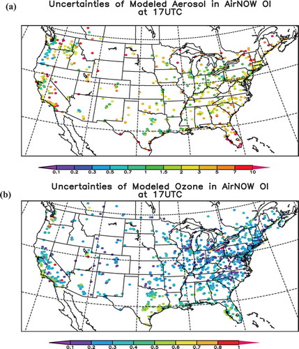
Figure 2 shows the relative uncertainties used in the OI4 case. For most areas, the aerosol uncertainty in the model ranged from 0.3 to 5.0. However, over Florida, the San Joaquin Valley of California, and the northwestern and northeastern states, the base model’s biases were relatively big. It is unclear why the base model had a larger bias over these places. Such large biases may be due to inaccurate emission, meteorology, or their combination. Liu et al. (2008) described a Saharan dust intrusion to the southeastern United States, which is common in the summertime, from satellite data. One possible reason for the model bias over Florida is the regional underestimation of this influx during summertime. In general, the base model performance over California needs to be improved. A similar situation is also applied to ozone, although ozone’s uncertainty is much lower than that of aerosols. Most regions have ozone uncertainty < 0.5.

Figure 2. Dynamic relative uncertainties for AIRNow OI used in OI4 case at 17 UTC: (a) aerosol and (b) ozone.

Results and Discussion

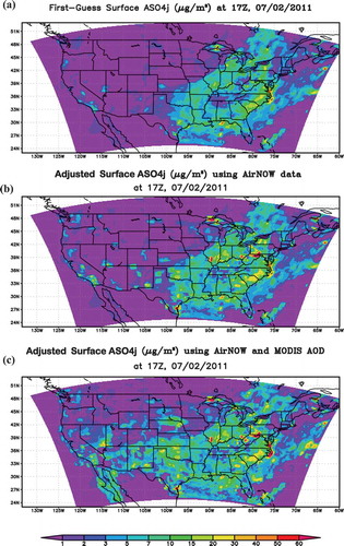
Figure 3 shows sulfate before and after assimilation in CMAQ’s accumulation mode from the OI4 case at 17Z, July 2, 2011. The first-guess result (OI4’s 14Z run) shows that sulfate aerosols were mostly distributed to the east of 100°W with a concentration <50 µg/m³. After the assimilation of AIRNow PM_2.5 data, some sulfate values >50 µg/m³ appeared in southeastern Illinois, northeastern West Virginia, and southern Pennsylvania. Since more than 65% of AIRNow PM_2.5 stations were in the Eastern USA (Figure 2), relatively sporadic adjustments are made for sulfate in the Midwest (Figure 3b). After we included MODIS data in the adjustment, areas including Arizona, New Mexico, western Texas, the Baja California Peninsula, and the Gulf of Mexico showed higher sulfates after OI (Figure 3c). However, over the eastern United States, the near-surface adjustment was mainly based on AIRNow measurements, since our method used available AIRNow assimilation to overwrite MODIS-based adjustment below the PBL.

Figure 3. Predicted and OI-assimilated surface accumulation-mode sulfate at 17Z, 07/02/2011: (a) the first-guess model (14Z OI4 run), (b) OI4 AIRNow OI only, and (c) OI4 AIRNow+MODIS OI.

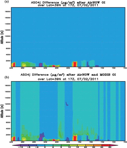
To illustrate the impact of assimilation, Figure 4 shows cross-sectional plots over 39°N from 90°W to 70°W. Figure 4a shows the accumulation-mode sulfate change with AIRNow-only OI from the 14Z simulation applied to layers within the PBL; the sulfate-concentration adjustment was up to 60 µg/m³, and all the adjustments were below 2 km. When MODIS OI was included (Figure 4b), the whole column changed if there was no AIRNow PM_2.5 observation nearby. Alternatively, the column changed above the PBL if an AIRNow PM_2.5 observation was available. In most areas, MODIS and AIRNow OI yielded a consistent trend of adjustment. For example, over 88°W, both data showed that the 14Z simulation underestimated aerosols, so OI increased sulfate below and above the PBL. A similar situation occurred over 85°W, where both adjustments decreased sulfate concentration. However, over 76.6°W, the two adjustments gave contradictory adjustment trends: AIRNow OI decreased sulfate, while MODIS OI increased sulfate. Although the two adjustments were applied below and above the PBL, respectively, thus avoiding direct conflict with each other in this study, more quality control for the observations and further study of aerosol’s vertical distribution are needed to address this contradiction. Unfortunately, these two sets of observation cannot give us information about aerosol’s vertical distribution.

Figure 4. Cross-section plot over 39°N of the accumulation-mode sulfate differences: (a) after AIRNow only OI, and (b) after AIRNow+MODIS OI (OI4 run).

Comparison to AIRNow measurements

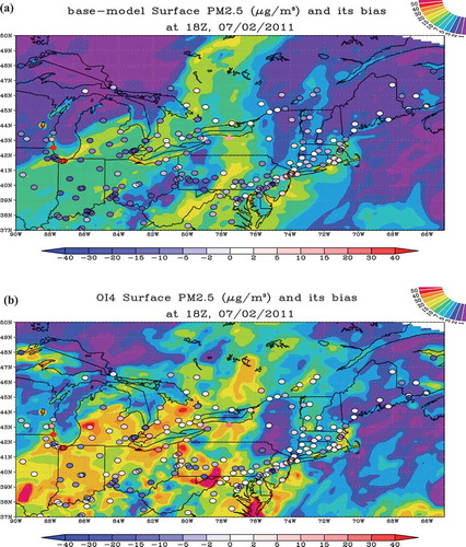
One of our goals was to generate a reasonable aerosol field comparable to AIRNow measurements. Figure 5 shows the base model and OI4 PM_2.5 biases over the northeastern United States at 18 UTC, that is, the first forecast hour from the 17 UTC assimilation. The base model underpredicted PM_2.5 over most regions, except for several stations near the Great Lakes. After the OI4 adjustment, the low biases were corrected over most areas, especially over the New England region, Indiana, Michigan, and Ohio. The high biases over the two stations near southeastern Wisconsin and northwestern Indiana near Lake Michigan persisted; since there were other nearby stations showing low or no biases, the OI method failed to adjust due to these contradictory signals. It should also be noted that we adjusted only the initial condition. Biases of emission and other persisting factors could quickly overwrite the correction, especially over polluted areas with relatively high emissions.

Figure 5. Predicted surface PM2.5 and its bias compared to AIRNow measurements in the base case (a) and OI4 (b) over the northeastern United States. The corner color bars show the predicted PM2.5, and the bottom color bars show the biases.

Figure 6a shows the time-series PM_2.5 plot for the base model and four OI cases. The base model without assimilation systematically underpredicted PM_2.5, especially during the daytime. The diurnal variation of PM_2.5 was relatively strong—high at night, and low during daytime—since the daytime convective PBL can pump the near-surface emission to higher altitudes, diluting aerosol concentrations. The AIRNow observations also showed a similar trend, but not as strong a diurnal variation as the base model result. All the OI runs tended to correct the underprediction. Among them, the OI4 case yielded the best performance and had relatively low daytime PM_2.5 bias. Assimilation performance is very sensitive to the uncertainty setting. Clearly the uncertainties decide the relative weighting between the model results and observations when analysis results are generated. The OI4 overpredicted PM_2.5 during the nighttime, except for midnight between July 4 and 5, when firework emissions contributed to high PM_2.5 during the night of Independence Day. The nighttime overprediction in the OI4 case could be caused by daytime overadjustment in the elevated layers or upwind areas, even though the 00Z and 06Z AIRNow OI brought down the bias a little bit. The base model’s ozone prediction was much better than that for PM_2.5 (Figure 6b), and the models agreed with the observations regarding the strong diurnal variation.

Figure 6. CMAQ base model and 4 OI runs compared to AIRNow surface PM2.5 over continental United States (a) and ozone over northeastern United States (b) (north of 37°N, east of 90°W).

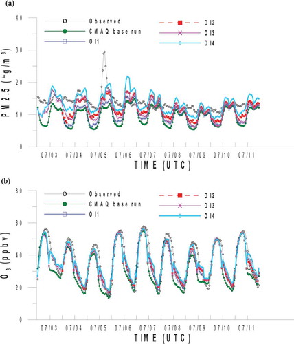
To highlight the effect of OI adjustment, Table 5 (shown later) shows the time-series O₃ plot over the northeastern United States instead of the continental United States. The ozone concentrations of the base model dropped faster than the observations after sunset, causing corresponding ozone underprediction. All the OI cases helped to correct this underprediction during the 00Z adjustment. The base model also underpredicted the ozone peak values on July 3, 4, and 8; the OI runs adjusted those underpredictions. All of the OI runs had similar performance for ozone, since the differences in uncertainty settings for ozone are not as big as those for PM_2.5. Table 4 shows the statistical results for a randomly selected 24-hr period, 12Z of July 6 to 12UTC of July 7, 2011. The base model’s performance for ozone was better than for PM_2.5. The assimilation’s improvements in O₃ correlation were not significant. Both the OI2 and OI4 cases included six adjustments per day, reducing the high O₃ biases by 1 ppbV. This result suggests that high-frequency adjustments are essential for greater improvement. The aerosol OIs showed similar results, as OI2 and OI4 were better than OI1 and OI3. Since the base model significantly underpredicted PM_2.5, the OI improvements were more obvious for this parameter. OI4 uses a dynamic uncertainty setting, which showed better results than OI2’s single-weighting uncertainty setting for modeled aerosol. Table 5 shows the same thing but for the southeastern states, where the base model had relatively poor performance, especially for PM_2.5. The OI method generally improved the correlation coefficient for both ozone and PM_2.5, though sometimes this method slightly increased mean bias. The OI4 improvement for PM_2.5 mean bias was more significant than the improvement shown in other cases, though its correlation coefficient still remained relatively low.

Table 5. Same statistics but for southeastern states (FL, GA, AL, MS, TN, SC, NC, VA, WV) from 12Z, 07/06/2011, to 12Z, 07/07/2011.

Cases ofstudies	O3 (ppbV)	PM2.5 (µg/m^3)
Base case	R = 0.55, MB = 0.22	R = 0.10, MB = –9.90
OI1	R = 0.58, MB = 0.43	R = 0.14, MB = –5.89
OI2	R = 0.61, MB = –0.85	R = 0.22, MB = –3.30
OI3	R = 0.58, MB = –1.40	R = 0.22, MB = –4.50
OI4	R = 0.60, MB = –0.59	R = 0.21, MB = –1.16

Comparison to aircraft measurements

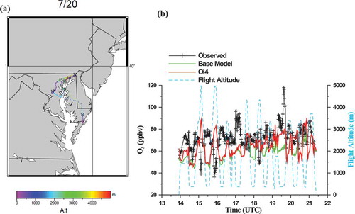
During July 2011, the NASA Discover-AQ field campaign took place around the Washington, DC and Baltimore region, with the P-3B aircraft measuring primarily gaseous chemical species (Crawford and Pickering, 2011). Here, we used aircraft-measured ozone to verify the impact of AIRNow OI on ozone simulation. Figure 7a shows the P-3B flight paths on July 20, 2011, colored by flight altitude and marked with UTC time. Figure 7b shows the results of the base model prediction and the OI4 case compared to airborne observations. For this flight, the base model generally underpredicted ozone below 1 km while overpredicting high-altitude (above 4 km) ozone around 15 and 16 UTC. The OI4 slightly corrected the high-altitude overpredictions and significantly improved the low-altitude underpredictions for the flight segment after 18UTC. Since our OI assimilation applied an ozone correction ratio to layers below the PBL based on assimilation of surface data from AIRNow, it is expected that the major change between the base model and OI would also be below the PBL where nearby AIRNow stations exist.

Figure 7. Discover-AQ 2011 P-3B flight on July 20: (a) flight path and (b) model/observed ozone comparison.

Figure 8 shows a comparison with another flight in this region on July 27, 2011. The base model overpredicted ozone at low altitudes on this day across the whole area. The OI4 case successfully corrected most of the low-altitude ozone overprediction, except for the flight segment of 15-17UTC; though OI4 also helped reduce this bias, it was not a strong enough correction. Figure 9 shows the O₃ correlations for 13 Discover-AQ flights below 2 km. The OI4 case improved O₃ simulation regarding both correlation coefficient and slope. Although we did not include aircraft data in the assimilation for any of the OI cases, these notable improvements demonstrate the success of AIRNow OI. Here we did not adjust the corresponding concentrations of NO_x and VOC, which are ozone precursors, due to the limited NO_x and VOC measurements. In principle, we should adjust all the related chemical species altogether to avoid chemical imbalance or instability. In our experience, the model can adapt that imbalance as the photochemical reactions can quickly reach new equilibrium. This process is similar to the air quality model adapting strong local NO_x and VOC emissions.

Figure 8. Discover-AQ P-3B flight on July 27: (a) flight path and (b) model/observed ozone comparison.

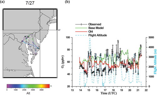
Figure 9. The base model (“o” symbol and solid fit line) and OI4 (“+” symbol and dash fit line) O₃ versus observation for 13 Discover-AQ P-3B flights (07/02/2011–07/29/2011) below 2 km.

Conclusion

In this study, we tested the assimilation method of optimal interpolation to adjust CMAQ’s initial conditions for July 2011 over the continental United States using AIRNow surface data and MODIS AOD. The performance of this assimilation depends on assimilation time frequency, station locations, vertical and horizontal extents, and parameter settings, such as uncertainties. The base model’s performance is also very important, especially when the model has certain systematic biases caused by various local factors, including meteorology and emissions. In this study, our base model systematically underpredicted daytime surface PM_2.5. Although the OI assimilation pushed the modeled concentration field toward the observations at four times (at 12Z, 14Z, 17Z, and 19Z in OI2 and OI4 cases) during daytime, somewhat correcting that aerosol underprediction, the correlation coefficients for PM_2.5 were still relatively low. Adjusting initial conditions alone may not be able to resolve this systemic bias, unless adjustments are made very frequently, such as hourly. Such high-frequency adjustment would effectively replace the model’s own predictions with observed data near the observation stations. The effect-lasting time of adjusted initial condition depends on many factors, such as the strength of local emission and of local wind. In our experience, stronger local emission could overwrite the OI impact faster than lower local emission. Strong wind over uneven polluted areas could also blow out the effect of adjusted local initial condition.

Some systematic biases for the dates in question were caused by faulty settings of the base model, such as missing the emissions of July 4 fireworks. Adjusting initial conditions, however, cannot fully correct these biases. The base model’s ozone prediction yields consistent diurnal variation except for the faster-than-real ozone decline after sunset in the northeastern United States. The OI runs can correct that bias if nearby observations are available. However, further study is still needed to address the physical causes of these biases.

Assimilation of ozone surface data improves not only the near-surface simulation but also low-altitude results below the PBL, as demonstrated by the comparison with the Discover-AQ aircraft data. In this study, we did not assimilate data from aircraft measurements, as they are only occasionally available. Using data from elevated levels in the assimilation could further improve the model. Here, MODIS AOD represented the loading of the aerosol column, and its retrieval quality can be affected by many factors. In this study, we used AIRNow PM_2.5 for aerosol assimilation below the PBL over the areas where nearby AIRNow PM_2.5 stations exist. MODIS AOD assimilation might conflict with AIRNow PM_2.5 assimilation, depending on modeled aerosol type, size, and vertical distribution. More studies are needed to address these uncertainties.

Funding

This study was partially supported by the NASA Earth Science Division’s Air Quality Applied Science Team (AQAST) project grant NNH14AX88I. The authors thank Professors Gregory Carmichael and Scott Spak of University of Iowa, Armistead Russell of George Tech., Dick McNider of Univeristy of Alabama, Yang Liu of Emory University, and Daniel Jacob of Harvard University for insightful guidance and advice. The authors also benefited tremendously from discussion by colleagues in the AQAST Chemical Analysis Tiger Team: David Edwards of NCAR, Edward Hyer of Naval Research Laboratory, Arastoo Pour Biazar of the University of Alabama, Yongtao Hu and Talat Odman of Georgia Tech, and Brad Pierce of NOAANESDIS/STAR.

Additional information

Funding

This study was partially supported by the NASA Earth Science Division’s Air Quality Applied Science Team (AQAST) project grant NNH14AX88I. The authors thank Professors Gregory Carmichael and Scott Spak of University of Iowa, Armistead Russell of George Tech., Dick McNider of Univeristy of Alabama, Yang Liu of Emory University, and Daniel Jacob of Harvard University for insightful guidance and advice. The authors also benefited tremendously from discussion by colleagues in the AQAST Chemical Analysis Tiger Team: David Edwards of NCAR, Edward Hyer of Naval Research Laboratory, Arastoo Pour Biazar of the University of Alabama, Yongtao Hu and Talat Odman of Georgia Tech, and Brad Pierce of NOAANESDIS/STAR.

Notes on contributors

Youhua Tang

Youhua Tang, Tianfeng Chai, Li Pan, Pius Lee, Daniel Tong, and Hyun-Cheol Kim are atmospheric scientists at the NOAA Air Resources Laboratory (ARL) and are also affiliated with the Cooperative Institute for Climate and Satellites at the University of Maryland in College Park, MD except Pius Lee. Daniel Tong is also affiliated to the Center for Spatial Information Science and System in George Mason University.

Tianfeng Chai

Youhua Tang, Tianfeng Chai, Li Pan, Pius Lee, Daniel Tong, and Hyun-Cheol Kim are atmospheric scientists at the NOAA Air Resources Laboratory (ARL) and are also affiliated with the Cooperative Institute for Climate and Satellites at the University of Maryland in College Park, MD except Pius Lee. Daniel Tong is also affiliated to the Center for Spatial Information Science and System in George Mason University.

Li Pan

Youhua Tang, Tianfeng Chai, Li Pan, Pius Lee, Daniel Tong, and Hyun-Cheol Kim are atmospheric scientists at the NOAA Air Resources Laboratory (ARL) and are also affiliated with the Cooperative Institute for Climate and Satellites at the University of Maryland in College Park, MD except Pius Lee. Daniel Tong is also affiliated to the Center for Spatial Information Science and System in George Mason University.

Pius Lee

Youhua Tang, Tianfeng Chai, Li Pan, Pius Lee, Daniel Tong, and Hyun-Cheol Kim are atmospheric scientists at the NOAA Air Resources Laboratory (ARL) and are also affiliated with the Cooperative Institute for Climate and Satellites at the University of Maryland in College Park, MD except Pius Lee. Daniel Tong is also affiliated to the Center for Spatial Information Science and System in George Mason University.

Daniel Tong

Youhua Tang, Tianfeng Chai, Li Pan, Pius Lee, Daniel Tong, and Hyun-Cheol Kim are atmospheric scientists at the NOAA Air Resources Laboratory (ARL) and are also affiliated with the Cooperative Institute for Climate and Satellites at the University of Maryland in College Park, MD except Pius Lee. Daniel Tong is also affiliated to the Center for Spatial Information Science and System in George Mason University.

Hyun-Cheol Kim

Youhua Tang, Tianfeng Chai, Li Pan, Pius Lee, Daniel Tong, and Hyun-Cheol Kim are atmospheric scientists at the NOAA Air Resources Laboratory (ARL) and are also affiliated with the Cooperative Institute for Climate and Satellites at the University of Maryland in College Park, MD except Pius Lee. Daniel Tong is also affiliated to the Center for Spatial Information Science and System in George Mason University.

Weiwei Chen

Weiwei Chen is an associate professor from the Northeast Institute of Geography and Agroecology, Chinese Academy of Sciences who visited NOAA/ARL in 2014.

References

- Adhikary, B., S. Kulkarni, A. Dallura, Y. Tang, T. Chai, L.R. Leung, Y. Qian, C.E. Chung, V. Ramanathan, and G.R. Carmichael. 2008. A regional scale chemical transport modeling of Asian aerosols with data assimilation of AOD observations using optimal interpolation technique. Atmos. Environ. 42(37):8600–15. doi:10.1016/j.atmosenv.2008.08.031
- Pour-Biazar, A., R.T. McNider, S.J. Roselle, R. Suggs, G. Jedlovec, D. W. Byun, S. Kim, C. J. Lin, T. C. Ho, S. Haines, B. Dornblaser, and R. Cameron. 2007. Correcting photolysis rates on the basis of satellite observed clouds. J. Geophys. Res. 112:D10302. doi:10.1029/2006JD007422
- Binkowski, F.S., and U. Shankar. 1995. The regional particulate model 1. Model description and preliminary results. J. Geophys. Res. 100(D12): 26191–26209. doi:10.1029/95JD02093
- Carmichael, G.R., A. Sandu, T. Chai, D.N. Daescu, E.M. Constantinescu, and Y. Tang. 2008. Predicting air quality: Improvements through advanced methods to integrate models and measurements. J. Comput. Phys. 227(7),3540–3571. doi:10.1016/j.jcp.2007.02.024
- Chai, T., G.R. Carmichael, A. Sandu, Y. Tang, and D. N. Daescu. 2006. Chemical data assimilation of Transport and Chemical Evolution over the Pacific (TRACE-P) aircraft measurements. J. Geophys. Res. 111:D02301. doi:10.1029/2005JD005883
- Crawford, J.H., and K. E. Pickering. 2011. DISCOVER-AQ observations over the Baltimore–DC area during July 2011. AGU Fall Meeting Abstracts, vol. 1.
- Dudhia, J. 1989. Numerical study of convection observed during the Winter Monsoon Experiment using a mesoscale two-dimensional model. J. Atmos. Sci. 46: 3077–3107. doi:10.1175/1520-0469(1989)046
- Foley, K.M., S.J. Roselle, K.W. Appel, P.V. Bhave, J.E. Pleim, T.L. Otte, R. Mathur, G. Sarwar, J.O. Young, R.C. Gilliam, C.G. Nolte, J.T. Kelly, A.B. Gilliland, and J. O. Bash. 2010. Incremental testing of the Community Multiscale Air Quality (CMAQ) modeling system version 4.7, Geosci. Model Dev. 3:205–26. doi:10.5194/gmd-3-205-2010
- Hong, S.-Y., Y. Noh, and J. Dudhia. 2006. A new vertical diffusion package with an explicit treatment of entrainment processes. Month. Weather Rev. 134:2318–41. doi:10.1175/MWR3199.1
- Hong, S.-Y., and J. Lim. 2006. The WRF single–moment 6–class microphysics scheme (WSM6). J. Korean Meteorol. Soc. 42:129–51.
- Liu, Z., A. Omar, M. Vaughen, J. Hair, C. Kittaka, Y. Hu, K. Powell, C. Trepte, D. Winker, C. Hostetler, R. Ferrare and R.B. Pierce. 2008. CALIPSO lidar observations of the optical properties of Saharan dust: A case study of long-range transport. J. Geophys. Res. 113(D7). doi:10.1029/2007JD008878
- Malm, W.C., J.F. Sisler, D. Huffman, R.A. Eldred, and T.A. Cahill. 1994. Spatial and seasonal trends in particle concentration and optical extinction in the United States. J. Geophys. Res. 99:1347– 1370. doi:10.1029/93JD02916
- Mathur, R., J. Pleim, K. Schere, G. Pouliot, J. Young, and T. Otte. 2005. The community Multiscale Air Quality (CMAQ) model: Model configuration and enhancements for 2006 air quality forecasting. Air Quality Forecaster Focus Group Meeting, September 16, 2005, Washington, DC.
- Mlawer, E.J., S.J. Taubman, P.D. Brown, M.J. Iacono, and S.A. Clough. 1997. Radiative transfer for inhomogeneous atmospheres: RRTM, a validated correlated–k model for the longwave. J. Geophys. Res. 102:16663–82. doi:10.1029/97JD00237
- Monin, A.S., and A.M. Obukhov. 1954. Basic laws of turbulent mixing in the atmosphere near the ground. Tr. Akad. Nauk SSSR Geofiz. Inst. 24.151:163–87.
- O’Neill, S. M., S. A. Ferguson, and R. Wilson. 2003. The BlueSky smoke modeling framework (www.blueskyrains.org). American Meteorological Society, 5th Symposium on Fire and Forest Meteorology, Orlando, FL.
- Pan, L., D. Tong, P. Lee, H.-C. Kim, and T. Chai. 2014. Assessment of NOx and O3 forecasting performances in the U.S. National Air Quality Forecasting Capability before and after the 2012 major emissions updates. Atmos. Environ. 95:610–19. doi:10.1016/j.atmosenv.2014.06.020
- Pierce, R.B., J.A. Al-Saadi, T. Schaack, A. Lenzen, T. Zapotocny, D. Johnson, C. Kittaka, M. Buker, M.H. Hitchman, G. Tripoli, T.D. Fairlie, J. R. Olson, M. Natarajan, J. Crawford, J. Fishman, M. Avery, E.V. Browell, J. Creilson, Y. Kondo, and S.T. Sandholm. 2003. Regional Air Quality Modeling System (RAQMS) predictions of the tropospheric ozone budget over East Asia. J. Geophys. Res. 108:8825. doi:10.1029/2002JD003176, D21
- Pleim, J.E. 2007. A combined local and nonlocal closure model for the atmospheric boundary layer. Part I: Model description and testing. J. Appl. Meteor. Climatol. 46, 1383–95. doi:10.1175/JAM2539.1
- Sarwar, G., et al. 2011. Impact of a new condensed toluene mechanism on air quality model predictions in the US. Geosci. Model Dev. 4:183–93, doi:10.5194/gmd-4-183-2011, 2011
- Sandu, A., T. Chai, and G.R. Carmichael. 2010. Integration of models and observations: A modern paradigm for air-quality simulations. Model. Pollut. Complex Environ. Systems 2:419.
- Segers, A. 2002. Data assimilation in atmospheric chemistry models using Kalman filtering. TU Delft, Delft University of Technology, Delft, The Netherlands.
- Tewari, M., et al. 2004. Implementation and verification of the unified NOAH land surface model in the WRF model. 20th Conference on Weather Analysis and Forecasting/16th Conference on Numerical Weather Prediction, Seattle, WA, January 2014, pp. 11–15.
- Tang, Y. 2002. A case study of nesting simulation for the Southern Oxidants Study 1999 at Nashville. Atmos. Environ. 36(10):1691–705. doi:10.1016/S1352-2310(02)00093-6
- Tang, Y., P. Lee, M. Tsidulko, H.-C. Huang, J.T. McQueen, G.J. DiMego, L.K. Emmons, R.B. Pierce, A.M. Thompson, H.-M. Lin, D. Kang, D. Tong, S.-C. Yu, R. Mathur, J.E. Pleim, T.L. Otte, G. Pouliot, J.O. Young, K.L. Schere, P.M. Davidson, and I. Stajner. 2009. The impact of chemical lateral boundary conditions on CMAQ predictions of tropospheric ozone over the continental United States. Environ. Fluid Mech. 9:43–58. doi:10.1007/s10652-008-9092-5
- Tong, D.Q., L. Lamsal, L. Pan, C. Ding, H. Kim, P. Lee, T. Chai, K.E. Pickering, and I. Stajner. 2015. Long-term NOx trends over large cities in the United States during the Great Recession: Comparison of satellite retrievals, ground observations, and emission inventories. Atmos. Environ. 107:70–84. doi:10.1016/j.atmosenv.2015.01.035
- Vukovich, J., and T. Pierce. 2002. The Implementation of BEIS-3 within the SMOKE modeling framework. Presented at “Emissions Inventories—Partnering for the Future,” the 11th Emissions Inventory Conference of the U.S. Environmental Protection Agency, Atlanta, GA, April 2002.
- Wang, Y., K. N. Sartelet, M. Bocquet, and P. Chazette. 2013. Assimilation of ground versus lidar observations for PM10 forecasting. Atmos. Chem. Phys. 13:269–83. doi:10.5194/acp-13-269-2013
- Wicker, L.J., and W.C. Skamarock. 2002. Time-splitting methods for elastic models using forward time schemes. Month. Weather Rev. 130:2088–97. doi:10.1175/1520-0493(2002)130
- Wu, L., V. Mallet, M. Bocquet, and B. Sportisse. 2008. A comparison study of data assimilation algorithms for ozone forecasts. J. Geophys. Res. 113:D20310, doi:10.1029/2008JD009991
- Zhang, D.-L., and R. A. Anthes. 1982. A high–resolution model of the planetary boundary layer: Sensitivity tests and comparisons with SESAME–79 data. J. Appl. Meteorol. 21:1594–609. doi:10.1175/1520-0450(1982)021