Analysis of alternative pathways for reducing nitrogen oxide emissions

Abstract

Strategies for reducing tropospheric ozone (O₃) typically include modifying combustion processes to reduce the formation of nitrogen oxides (NO_x) and applying control devices that remove NO_x from the exhaust gases of power plants, industrial sources and vehicles. For portions of the U.S., these traditional controls may not be sufficient to achieve the National Ambient Air Quality Standard for ozone. We apply the MARKet ALlocation (MARKAL) energy system model in a sensitivity analysis to explore whether additional NO_x reductions can be achieved through extensive electrification of passenger vehicles, adoption of energy efficiency and conservation measures within buildings, and deployment of wind and solar power in the electric sector. Nationally and for each region of the country, we estimate the NO_x implications of these measures. Energy efficiency and renewable electricity are shown to reduce NO_x beyond traditional controls. Wide-spread light duty vehicle electrification produces varied results, with NO_x increasing in some regions and decreasing in others. However, combining vehicle electrification with renewable electricity reduces NO_x in all regions.

Implications: State governments are charged with developing plans that demonstrate how air quality standards will be met and maintained. The results presented here provide an indication of the national and regional NO_x reductions available beyond traditional controls via extensive adoption of energy efficiency, renewable electricity, and vehicle electrification.

Introduction

National Ambient Air Quality Standards (NAAQS) specify maximum allowable air pollutant concentrations in the United States. The 8-hr NAAQS for tropospheric ozone (O₃), a principal component of photochemical smog, was set at 75 ppb in 2008 (Federal Register, 2008). State air quality agencies are charged with developing State Implementation Plans (SIPs) to bring nonattainment areas into attainment with the standard. Since O₃ is formed through a photochemical reaction involving nitrogen oxides (NO_x) and volatile organic compounds (VOCs), and since this reaction is limited by NO_x in most parts of the country, O₃ SIPs typically focus on reducing NO_x.

State actions related to SIPs, combined with a range of federal regulations, have reduced U.S. NO_x emissions by 51% from 1990 to 2014 (U.S. Environmental Protection Agency [EPA], 2015a). Over that period, electric sector NO_x was reduced by 73% and on-road vehicle NO_x by 53%. The majority of these reductions have been achieved by modifying combustion processes and placing control devices on the exhaust systems of stationary and mobile sources. For example, many coal-fired electric utilities reduce emissions via low-NO_x burners (LNB) and selective catalytic reduction (SCR) systems, and modern passenger cars and trucks are fitted with catalytic converters.

One approach for developing an O₃ SIP is to estimate the NO_x reductions that could be achieved through greater application of traditional controls, such as LNB and SCR. The state’s emission inventory is modified to reflect the additional controls, and air quality modeling is conducted to estimate whether the standard would be met. The control strategy then can be refined iteratively to hone in on a cost-effective solution. To support SIP efforts, the EPA produces a “Menu of Control Measures” (EPA, 2012) and maintains and distributes a database of control characterizations, the Control Measures Database (EPA, 2014c).

The O₃ NAAQS poses challenges for this methodology. Previous analysis of strategies to meet the O₃ NAAQS suggests that reductions achievable from traditional controls may not yield attainment in some portions of the country (EPA, 2008). Although history indicates that regulations can be drivers for the development of new controls (Saha et al., 2005), there also may be opportunities to incorporate alternative, nontraditional emission reduction measures into the SIP. Examples include renewable electricity, energy efficiency, and fuel switching. These measures generally are not considered in SIPs and other air quality management strategies because limited tools are available to evaluate their emission reduction potential and cost-effectiveness.

The EPA MARKet ALlocation (MARKAL) modeling framework now has the capability to provide insights regarding the regional emission reduction potential of these measures. In this paper, we present a sensitivity analysis in which we demonstrate the application of MARKAL to estimate NO_x reductions available at the U.S. Census Division level via extensive adoption of renewable electricity, energy efficiency, or fuel switching after currently characterized traditional controls have been exhausted. Although these alternative measures will also affect emissions of other pollutants, including sulfur dioxide (SO₂), directly emitted particles (PM_2.5 [particulate matter with an aerodynamic diameter <2.5 μm]), and climate pollutants such as carbon dioxide (CO₂), we present results only for NO_x, leaving the co-pollutant impacts for further research. These results can provide planners with an indication of the relative efficacy of each measure in reducing NO_x within their region. Furthermore, this application provides a blueprint that can be replicated using energy system models with a higher degree of spatial resolution. As this is a sensitivity analysis, our focus is on the direction and magnitude of emission changes and not on cost-effectiveness. Cost-minimizing strategies would potentially include a blend of traditional controls and alternative control measures, and may not exhaust either type of control measure. However, for the purposes of this exploration, we assume that traditional controls have been exhausted first before alterative controls are applied. In ongoing research, we are evaluating the costs of these alternative measures, comparing them with traditional controls, and identifying optimal levels of adoption of both traditional and alternative measures, including consideration of reductions in co-pollutants.

Background

Renewable electricity, energy efficiency, and fuel switching have garnered interest as means to mitigate greenhouse gases while simultaneously reducing traditional air pollutant emissions (e.g., Tonn and Paretz, 2007; Sioshansi and Denholm, 2009; Rao et al., 2013; Intergovernmental Panel on Climate Change [IPCC], 2014). From the federal and state air quality planning perspectives, these measures have the potential to complement more traditional controls in air quality management strategies (State and Territorial Air Pollution Program Administrators/Association of Local Air Pollution Control Officials [STAAPPA/ALAPCO], 1999; Haberl et al., 2004). However, the efficacy of particular measures is dependent on underlying location-specific factors, such as the emission intensity of the existing electricity production, access to renewable resources, and local and regional environmental policies (Michalek et al., 2011).

Since the assessment of the emission impacts of these measures is complex, computational tools and models have been used (U.S. EPA, 2011). A limited number of such tools and models are available, however. One option is the EPA’s AVoided Emissions and geneRation Tool (AVERT), which quantifies the emission implications of energy efficiency and renewable energy based upon a statistical analysis of recent electricity production data (EPA, 2014a). In its current form, reductions in energy demands must be determined exogenously. Furthermore, AVERT is not intended to be applied to assess years more than 5 years beyond the baseline data and therefore is not appropriate for longer-term planning.

Another option is the National Energy Modeling System (NEMS) (U.S. Energy Information Administration [EIA], 2009), which is used by the U.S. EIA to develop the Annual Energy Outlook (AEO; U.S. EIA, 2014). NEMS represents the entire U.S. energy system, which stretches from the import or extraction of energy through its use in meeting society’s energy demands. Thus, the system includes coal mines, oil and gas wells, refineries, electric power plants, manufacturing and other industries, space conditioning and lighting options in commercial and residential buildings, and various modes of transportation. As NEMS has primarily been used for energy planning, its characterization of air pollutant emissions and controls is limited.

The EPA MARKet ALlocation (MARKAL) modeling framework is an alternative to NEMS. EPA MARKAL consists of the MARKAL energy system model (LouLou et al., 2004) and the EPA nine-region MARKAL database (EPA, 2013). Like NEMS, the EPA MARKAL framework can be used to evaluate the technology and fuel implications of energy system scenarios, albeit in a more simplified, linearized representation (EPA, 2013). Unlike NEMS, the EPA MARKAL framework has energy system-wide coverage of many greenhouse gas and air pollutant emission factors, and includes representations of traditional emission controls, such as LNB and SCR for NO_x, flue gas desulfurization for sulfur dioxide (SO₂), and electrostatic precipitators and fabric filters for particulate matter (PM). The framework has been applied to assess the emission implications of energy scenarios (e.g., Loughlin et al., 2011; Akhtar et al., 2013), in energy technology and fuel assessments (e.g., Gullet et al., 2012; Loughlin et al., 2012), and to identify energy pathways that meet air quality, climate, and energy goals (Balash et al., 2013; Brown et al., 2013).

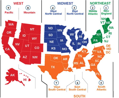
A drawback of the EPA MARKAL framework for application to SIPs is its spatial resolution, shown in Figure 1. This resolution requires that state-level policies and pollution control strategies be aggregated to the U.S. Census Division level. Although outputs can be used to identify important regional conditions and trends in parts of the country, these results may be less representative of individual states within each region and of the nonattainment areas within those states.

Figure 1. U.S. Census Divisions. Corresponding MARKAL region numbers are shown in circles above each division name. Adapted from the U.S. Energy Information Administration.

The Northeast States for Coordinated Air Use Management (NESCAUM) has developed Northeast-MARKAL, or NE-MARKAL, which covers 11 states plus the District of Columbia (Goldstein et al., 2008). Two Northeast states have expressed interest in exploring the use of this model to inform their upcoming O₃ SIP processes, focusing on the evaluation of renewable energy and energy efficiency measures (NESCAUM, 2014). Although NE-MARKAL can be modified to incorporate additional states, this process is time-consuming and is complicated by the limited availability of state-level energy system data.

With the goals of providing national coverage and demonstrating regional insights, we selected the EPA MARKAL framework for this study. This framework and study methodology are discussed in more detail in the following section.

Methodology

MARKAL model

MARKAL is a linear programming model that is composed of constructs such as energy carriers, process technologies, demand technologies, and energy service demands. The EPAUS9r_14_v1.2 MARKAL database allows the model to simulate the evolution of the U.S. energy system over the period spanning from 2005 through 2055, in 5-yr increments, and at the spatial resolution of the nine U.S. Census Divisions.

MARKAL operates by selecting the technologies and fuels that meet projected energy demands over the entire time horizon at least cost. Technology and fuel selections take into account complex factors such as the competition for fuels among sectors of the energy economy (e.g., the electric, industrial, residential, commercial, and transportation sectors compete for natural gas) and the diurnal patterns of various energy supplies and demands (e.g., solar photovoltaics generate electricity during the day, but residential heating demands are greatest at night). In the context of air quality management and greenhouse gas mitigation, constraints can be added to represent single or multipollutant emission limits. MARKAL then explicitly accounts for these constraints while optimizing.

The primary source of energy resource, technology, and demand data is the 2014 version of the AEO (AEO14). The spatial resolution by which these energy system components are represented is the U.S. Census Division. Technology- and fuel-specific emission factors are included for NO_x, SO₂, carbon monoxide (CO), volatile organic compounds (VOCs), PM less than 2.5 microns in diameter (PM_2.5), carbon dioxide (CO₂), nitrous oxide (N₂O), black carbon (BC), and organic carbon (OC). These factors are obtained from the EPA’s WebFire emission factor database (EPA, 2014e), Greenhouse Gas Inventory (EPA, 2010a), and MOtor Vehicle Emissions Simulator (MOVES; EPA, 2010b), as well as from Argonne National Laboratory’s Greenhouse gases Regulatory Emissions and Energy use in Transportation (GREET) model (Wang et al., 2007).

The Business as Usual (BAU) scenario used in this analysis has been calibrated to produce similar fuel use projections as in the AEO14 Reference Case (EIA, 2014). BAU also captures relevant on-the-books air quality regulations, including the Clean Air Interstate Rule (CAIR; Federal Register, 2005) and the Mercury and Air Toxics Standards (MATS) rule (Federal Register, 2011). On-road mobile emission factors are adjusted to approximate the effects of the Tier 3 standards (EPA, 2014d). To validate the BAU emission projection, regional, sector-specific emissions in 2010 and 2025 are compared with those of the EPA 2011 emission modeling platform (EPA, 2014h) and the 2025 projection developed for the recent Regulatory Impact Analysis (RIA) of a revised NAAQS (EPA, 2014f, 2014g). BAU is similar to the Base Case scenario that is distributed with EPAUS9r_2014_v1.2, with the exception that a constraint has been added to approximate greenhouse gas emissions implications of the Regional Greenhouse Gas Initiative (RGGI) (2013).

Note that the U.S. Court of Appeals lifted the stay on the Cross-State Air Pollution Rule (CSAPR) in 2014, resulting in CSAPR replacing CAIR (U.S. Court of Appeals, 2014). This change is not reflected in the MARKAL modeling conducted here. However, an examination of the electric sector modeling conducted by EPA to evaluate these rules suggests similar levels of regional NO_x reductions (EPA, 2015b). We do not believe that inclusion of CSAPR in BAU would result in substantial changes to modeling results. Also, the Clean Power Plan proposal (EPA, 2014b) is not incorporated into the BAU as the rule had not been finalized when this analysis was conducted.

Experimental approach

“Sensitivity analysis” has multiple definitions in the literature (Saltelli et al., 2008). We refer to sensitivity analysis as the evaluation of changes in the outputs of a model in response to incremental perturbations to the inputs to the model. The set of original inputs and outputs is the baseline, and each incrementally modified variant is a sensitivity run. Sensitivity analysis differs from scenario analysis, which commonly involves the simultaneous modification of multiple model inputs and parameters to correspond to wide-ranging narratives of the future (Schoemaker, 1991; Schwartz, 1997).

We apply sensitivity analysis to examine how national and regional technology selections, fuel use, and, ultimately, emissions respond to the assumptions about the increased levels of adoption of energy efficiency, vehicle electrification, and renewable electricity. First, we use the BAU scenario as the baseline and evaluate how outputs change with the application of maximum traditional NO_x controls in the electric, industrial, residential, commercial, and transportation sectors. Maximum traditional controls reflect the currently available information on combustion process changes and postcombustion controls, and may not reflect all of the potential controls that may be developed in future years. This sensitivity run is referred to as MaxCntl.

Next, we use MaxCntl as a new baseline and evaluate the response to the following, both individually and in combination:

• Energy efficiency (EE)—Increased application of energy efficiency and conservation measures in buildings

• Vehicle electrification (VE)—Increased light-duty vehicle electrification, including both full electric vehicles and plug-in hybrids

• Renewable electricity (RE)—Increased deployment of wind and solar technologies for electricity production

Incremental application of these constraints results in the MaxCntl+EE, MaxCntl+VE, and MaxCntl+RE sensitivity runs. The combination MaxCntl+VE+RE examines whether forcing renewable electricity improves the emission reduction potential of vehicle electrification, MaxCntl+EE+RE explores whether the emission reductions from benefits of energy efficiency diminish with high penetrations of renewable electricity, MaxCntl+VE+EE evaluates whether energy efficiency can offset the increased electricity demands of vehicle electrification, and MaxCntl+RE+VE+EE combines all three sets of assumptions. Table 1 lists BAU, MaxCntl, and the seven sensitivity runs that are evaluated.

Table 1. Sensitivity runs that are evaluated

Code	Short Description
BAU	Business as usual scenario
MaxCntl	Maximum NOx removal efficiency control devices are used on electric sector, industrial, residential, commercial, and off-highway sources
MaxCntl+EE	Increased employment of energy efficiency assumptions are added to MaxCntl
MaxCntl+VE	Increased employment of vehicle electrification assumptions are added to MaxCntl
MaxCntl+RE	Increased employment of renewable energy assumptions are added to MaxCntl
MaxCntl+EE+RE	Both increased employment of energy efficiency and renewable energy are added to MaxCntl
MaxCntl+EE+VE	Both increased employment of energy efficiency and vehicle electrification are added to MaxCntl
MaxCntl+VE+RE	Both increased employment of vehicle electrification and renewable energy are added to MaxCntl
MaxCntl+EE+VE+RE	All three measures are added to MaxCntl

Derivation of assumptions

The derivations of the MaxCntl, EE, VE, and RE are described below. See Supplemental Material for more detailed descriptions of their derivations. We attempt to keep these sensitivity assumptions aggressive yet plausible by basing them upon optimistic technological scenarios found in the literature. As our analysis is intended to be a sensitivity exercise, we do not consider the policy or regulatory levers that would be necessary to implement such assumptions.

MaxCntl approximates the emission reductions possible if electric sector coal boilers, industrial emissions sources, residential and commercial emission sources, and off-road engines employ the highest removal efficiency control options available. For the electric sector, this requirement implies that all coal-fired boilers use SCR, and that the SCR controls are run continuously throughout the year. For industrial, residential, commercial, and off-road sectors, control data are derived from the Control Measures Database used for the O₃ NAAQS RIA proposal. No controls beyond the Tier 3 requirements are considered for the on-road, air, marine, and rail transportation subsectors, although these controls may be considered in future work. Average percent reduction and cost per ton of pollutant treated for controls are calculated within each MARKAL region and source category. These controls are applied to all relevant sources from 2020 onward.

EE comprises a variety of assumptions and constraints. For example, heating and cooling demand reductions are obtained from the AEO14 Best Available Demand Technology Case (U.S. EIA, 2014). The efficiencies of miscellaneous electricity and office technologies increase by 0.5% in 2020 and 15% in 2030. In the residential and commercial sectors, the model is allowed to purchase only high-efficiency technologies in 2015, and only the most efficient technologies by fuel type starting in 2020. The use of residential and commercial solar photovoltaics increases in accordance with the AEO14 Best Available Demand Technology Case. Finally, lower bounds on the market share of electricity in space and water heating are increased from AEO14 Reference Case levels, resulting in additional electrification of these end uses. For example, in the residential sector, electric space heating has a 22% market share from 2035 onward in BAU, but this percentage is increased to 35% with the addition of EE. We do not currently consider energy efficiency measures in the industrial sector, but the analysis could be expanded to include these in the future.

VE assumptions are derived from the Lawrence Berkeley National Laboratory report “Scenarios for meeting California’s 2050 climate goals” (Wei et al., 2013). This report includes zero-emission vehicle (ZEV) penetration projections consistent with the “Governor’s ZEV Plan for California” (State of California, 2013), as well as a more intensive electrification scenario. We use the latter because it leads to a higher degree of electrification by 2035, which is near the end of the time period considered in NAAQS attainment planning. The scenario is assumed to be implemented nationwide. Electrification options are not considered for heavy-duty trucks or other non-light-duty vehicles in this analysis.

RE assumptions are developed from the National Renewable Energy Laboratory (NREL) Renewable Electricity Futures Study (NREL, 2012). In that study, several pathways were developed for achieving 80% renewable electricity production by 2050. We use the Incremental Technology Improvement scenario (RE-ITI) to obtain state-level wind and solar generation levels. These levels are aggregated to the EPA MARKAL regions, the U.S. Census Divisions, and MARKAL is forced to produce at least this total quantity electricity from wind and solar energy.

Results and Discussion

In this section, each sensitivity run is compared with MaxCntl to examine implications for NO_x and other pollutants. Although most results are shown through 2050, we highlight results in 2035 to illustrate various trends and sectoral interactions. The year 2035 was selected because the controls specified in MaxCntl and the assumptions outlined in EE, VE, and RE would be nearly fully realized by that year. Furthermore, 2035 is still policy-relevant from a SIP perspective, but has less uncertainty in the underlying drivers that affect emissions than subsequent years.

To facilitate comparison of the sensitivity runs with MaxCntl, we provide a set of summary graphics in Supplemental Material. These graphics include electricity production by fuel; light-duty vehicle technology penetration; residential, commercial, and industrial fuel consumption; sectoral NO_x; and the system-wide trajectories for NO_x, CO₂, SO₂, and PM_2.5.

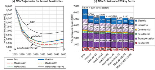
NO_x trajectories for BAU, MaxCntl, and select sensitivity runs are shown in Figure 2a, with sectoral breakouts for 2035 in Figure 2b. The Resource sector includes oil, natural gas, and coal extraction and processing. The downward trend through 2035 in BAU illustrates the effectiveness of the existing regulations that target NO_x. The trend is reversed after 2035, however, as energy demands increase to account for projected population and economic growth. MaxCntl reduces NO_x by approximately 13–16% per year from 2020 onward. Most of the sensitivity runs produce additional reductions, with the exception of MaxCntl+VE, in which NO_x levels are relatively unchanged from MaxCntl.

Figure 2. National system-wide and sectoral NO_x emissions under BAU, MaxCntl, and other sensitivity runs. (a) Illustrates the national-scale NO_x emission trajectories for several sensitivities through 2050. (b) Compares their sectoral NO_x emissions in 2035, illustrating key sectoral differences from one sensitivity to another.

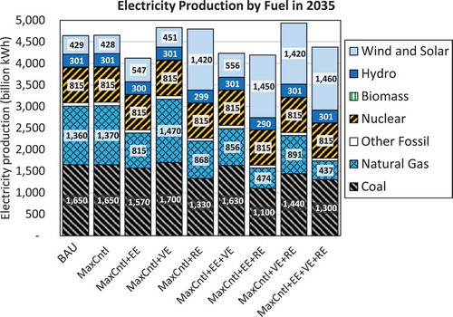
Of the sectoral emissions in 2035, electric sector NO_x shows the greatest variability from one sensitivity run to another. Figure 3 shows electricity production by fuel for each sensitivity run. The results in Figures 2b and 3 suggest a high degree of correlation (0.97) between coal-fired electricity production and electric sector NO_x. Conforming to this relationship, MaxCntl+EE+RE has the lowest electricity production from coal-fired boilers (1100 billion kWh) and also the lowest electric sector NO_x (655 thousand tons).

Figure 3. National electricity production by fuel in 2035 for each sensitivity run. Total electricity production in 2035 differs from one scenario to another, driving the differences in electric sector emissions depicted in Figure 2.

NO_x implications of adding EE, VE, and RE constraints individually

Examining differences in sectoral NO_x between MaxCntl and selected sensitivity runs helps provide insights into the results above. Figure 4 shows differences between MaxCntl and BAU, as well as between MaxCntl and MaxCntl+RE, MaxCntl+VE, MaxCntl+EE, and MaxCntl+EE+VE+RE.

Figure 4. National NO_x emissions changes by energy system sector, comparing MaxCntl with BAU and various sensitivity runs. (a) Compares MaxCntl and BAU, indicating the quantity of NO_x reductions by sector upon application of emission controls. (b–e) Compare selected sensitivities with MaxCntl, indicating additional reductions that occur.

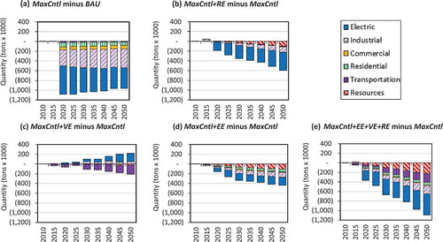
Compared with BAU, MaxCntl reduces electric sector and industrial NO_x by roughly equivalent amounts, whereas considerably smaller reductions are achieved from other sectors (Figure 4a). Adding RE to MaxCntl reduces overall NO_x, with the electric sector dominating these reductions; however, there are additional reductions in the industrial and resource sectors (see Figure 4b). EE yields roughly equivalent reductions in the electric, industry, and resource sectors, with smaller reductions coming from the residential and commercial sectors (see Figure 4d). The response to the addition of VE is more complicated: transportation and commercial sector emissions decrease, but electric and industrial sector emissions increase (see Figure 4c). At the national scale, the net result is very little change. We delve into these various responses in more detail below.

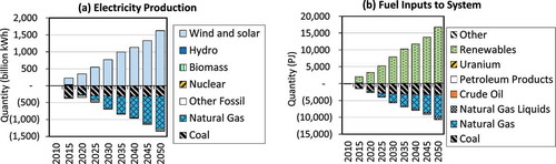
Figure 5 illustrates how electricity production and system-wide fuel use change when RE is added to MaxCntl. Overall, electricity production increases, reflecting fuel switching to electricity in the end-use sectors (Figure 5a). Direct NO_x emissions from those sectors decline slightly as a result. At the same time, MARKAL opts to offset a portion of the increased wind and solar power by lowering electricity production from natural gas and coal (Figure 5b). Thus, electric sector NO_x is reduced as well. With fuel switching away from fossil fuels, overall coal mining and natural gas extraction activities decrease, accounting for NO_x reductions in the resource sector.

Figure 5. National electricity production changes when RE is added to MaxCntl. (a) Indicates a net increase in electricity production, with wind and solar power increases being larger than decreases in generation from coal and natural gas. (b) Shows that decreases in gas and coal are energy system-wide. Changes in the use of other fossil fuels are very small in comparison.

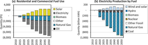
Figure 6 shows that adding EE to MaxCntl decreases residential and commercial energy demands, lowering both fossil fuel and electricity use in those sectors (Figure 6a). Thus, there are both sectoral and upstream (e.g., from electricity production) NO_x reductions that result. Upstream NO_x reductions are magnified by MARKAL’s decision to decrease electricity production from natural gas turbines and coal boilers (Figure 6b).

Figure 6. National residential and commercial fuel use, as well as changes in electricity production in the electric sector, when EE is added to MaxCntl. (a) Shows that EE results in a net decrease in residential and commercial fuel use. (b) Indicates the reduction in end-use energy electricity demand results in reduced electricity production from natural gas and coal.

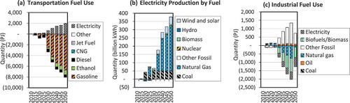
Figure 7 provides clues about the dynamics underlying the increase of industrial NO_x when VE is applied. As electricity demands increase in the light-duty transportation sector, gasoline use decreases substantially (Figure 7a). At the same time, the additional electricity for vehicles is being produced by a mix of fuels, with natural gas seeing the greatest increase (Figure 7b). Coal-fired electricity production also increases after 2020, as MARKAL opts to extend the lifetimes of existing coal plants. Wind and solar output grows after 2030. Together, these changes increase the market price of electricity and decrease the price of petroleum products. Industry responds accordingly, increasing its use of petroleum products. Industrial NO_x emissions increase as a result (Figure 7c).

Figure 7. National transportation fuel use, electricity production, and industrial fuel use changes in response to adding VE to MaxCntl. (a) Shows that the net fuel use by the transportation sector decreases with VE. (b) Indicates that the increased electricity demand is primarily being met by natural gas, although coal plant output increases, as does output from wind and solar. (c) Represents industrial sector fuel use, which appears to decrease while also transitioning from gas and biomass to other fossil fuels such as liquefied petroleum gas (LPG).

NO_x implications of adding combinations of the EE, VE, and RE constraints

The results and discussion above examine application of EE, VE, and RE individually. Next, we examine combinations of EE, VE, and RE. Questions that we explore include “Does introducing RE negate the NO_x benefits of EE?” “Does introducing RE compound the benefits of VE?” and “To what extent are the NO_x benefits of RE, EE, and VE benefits additive?”

To address these questions, we compare the 2035 NO_x totals for each sensitivity run (Figure 2b). Adding EE to MaxCntl reduces NO_x by an additional 280 thousand tons, whereas adding RE to MaxCntl reduces NO_x by 340 thousand tons. Applying these measures together reduces 620 thousand tons, equivalent to the sum of the two measures applied individually. Thus, at least on the national scale, RE and EE appear to be roughly additive. However, adding VE to MaxCntl+EE+RE does not produce additive benefits, and NO_x increases in 2035 by 10 thousand tons in response.

Next, we examine the dynamics associated with pairing VE with RE. Figure 2b indicates that adding VE to MaxCntl reduces an additional 10 thousand tons of NO_x nationally in 2035, making it the least effective of the three alternative measures. In contrast, adding RE to MaxCntl yields an additional NO_x reduction of 340 thousand tons. When VE and RE are combined, however, 370 thousand tons of NO_x are reduced. Thus, benefits of VE are tripled when RE is also applied, since the additional electricity production has a much lower NO_x intensity.

Similarly, the results suggest that there is a benefit of combining VE with EE. Figure 3 shows that VE alone results in MARKAL choosing to increase electricity production from coal and natural gas. However, adding EE to MaxCntl+VE more than offsets the VE electricity demands. With lower electricity demand relative to MaxCntl, MARKAL is able to decrease electricity production from coal and natural gas, lowering the NO_x intensity of electricity. As a result, the combination of VE and EE reduces 330 thousand tons in 2035, even though the sum of their individual reductions is 290 thousand tons.

Regional emission responses

The results shown to this point are at the national level. Table 2 lists the national and regional percent reductions of NO_x in 2035 associated with each sensitivity run. Results for select sensitivity runs are also shown graphically in Supplemental Material. For MaxCntl, percent reductions are relative to BAU, whereas all other sensitivity runs are compared with MaxCntl.

Table 2. Percent NO_x reductions in 2035 for each sensitivity run. For MaxCntl, percent reductions are relative to BAU, whereas all other reductions are relative to MaxCntl. Negative values imply a reduction

Sensitivity	National	R1	R2	R3	R4	R5	R6	R7	R8	R9
MaxCntl	−16%	6%	−20%	−17%	−18%	−14%	−20%	−14%	−20%	−11%
MaxCntl+EE	−5%	−22%	−10%	−3%	−2%	−6%	−6%	−4%	−5%	−4%
MaxCntl+VE	0%	13%	4%	−5%	0%	1%	0%	−1%	0%	−4%
MaxCntl+RE	−6%	−16%	−10%	−4%	−12%	−5%	−6%	−3%	−7%	−8%
MaxCntl+EE+VE	−6%	−20%	−7%	−9%	−2%	−4%	−8%	−4%	−4%	−9%
MaxCntl+EE+RE	−12%	−23%	−15%	−8%	−15%	−15%	−11%	−7%	−12%	−12%
MaxCntl+VE+RE	−7%	−13%	−8%	−8%	−11%	−2%	−7%	−4%	−6%	−13%
MaxCntl+EE+VE+RE	−11%	−22%	−14%	−13%	−14%	−8%	−9%	−7%	−11%	−17%

Many of the same trends witnessed at the national level are evident in MARKAL’s regional NO_x projections. For example, in seven of the nine regions, MaxCntl+EE+RE produces the greatest NO_x reductions. Only in Region 3 (East North Central) and Region 9 (Pacific) is MaxCntl+EE+RE surpassed by MaxCntl+EE+RE+VE. Whereas MaxCntl+VE produced mixed results across regions, combining MaxCntl+VE+RE yielded NO_x reductions in all regions.

Nonetheless, there are some distinct differences from region to region. For example, MaxCntl+EE+RE NO_x reductions range from 23% in Region 1 (New England) to only 7% in Region 7 (West South Central), whereas MaxCntl+VE reduces NO_x by 5% in Region 3 (East North Central) but increases NO_x by 13% in Region 1. Regional differences are also evident when we identify which individual measure results in the highest reduction regionally. For example, EE reduced the greatest percentage of emissions in Regions 1, 5 (South Atlantic), and 7. In contrast, RE reduced the greatest percentages in Regions 4 (West North Central), 8 (Mountain), and 9 (Pacific), and VE reduced the greatest percentage in Region 3.

Although examining root causes for regional differences is the subject of ongoing work, we hypothesize that access to renewable electricity and the emission intensity of the existing electric sector are important factors. Interregional trading of fuels and electricity, as well as the existence of regional emission limits imposed by CAIR and RGGI, also likely influences such decisions.

Conclusion

Traditional NO_x controls, such as LNB and SCR, may not be sufficient to meet the 2008 O₃ NAAQS in some parts of the country. Current tools and methods for exploring nontraditional emission reduction measures have not been generally available. We address this limitation by demonstrating how the EPA MARKAL energy modeling framework can be applied in a sensitivity analysis to examine the emission reduction potential of energy efficiency (EE), light-duty vehicle electrification (VE), and renewable electricity (RE). This modeling suggests that maximum application of traditional NO_x controls reduces 2035 national energy-system NO_x emissions by 16% relative to BAU. The addition of EE, VE, and RE can reduce NO_x by another 10% relative to BAU.

Modeling results also highlight the benefits of applying an energy system model that is able to identify potentially important cross-sector interactions. For example, adding VE to MaxCntl affected vehicle and electricity production emissions as expected: vehicle emissions decreased, whereas electric sector emissions increased to a lesser degree. However, the resulting fuel price pressures led to an increase in industrial emissions. In some regions, overall NO_x emissions increased. A direction of future research could be to understand this response more fully and whether it could be expected in the real world or whether it is an artifact of the simplifications inherent in modeling. This knowledge could be very useful in the design of effective and robust air quality management strategies. Another critical finding is that there can be synergies among EE, VE, and RE measures. For example, several combinations of EE, VE, and RE are shown to produce more reductions than the sum when applied individually.

For many regions of the country, the combination of EE and RE yields the greatest NO_x reductions. The performance of each measure is shown to vary regionally, however, and the selection of the most effective strategy for achieving NO_x reductions should take into account a wide variety of regional factors. We are exploring the drivers for regional differences in ongoing work, including the effects of existing technology stock, competition for fuels among sectors, access to low-cost renewables and natural gas, regional air pollutant, and greenhouse gas emission limits.

A number of extensions to this work are ongoing or planned. For example, we expect to update the BAU to reflect more recent air and climate regulations after they are promulgated. Additional refinements may include the following: expanding vehicle electrification to include medium- and heavy-duty trucks, rail and marine vehicles; incorporating industrial energy efficiency into EE; and revising the analysis to consider seasonal emissions and control operation. Furthermore, we are evaluating the impacts of each measure on co-emitted pollutants, including other air pollutants, short-lived climate pollutants, and greenhouse gases. Reductions in co-emitted pollutants can be substantial. For example, adding EE, VE, and RE to MaxCntl reduces national SO₂, PM_2.5, and CO₂ emissions in 2035 by 2%, 12%, and 21%, respectively (see Supplemental Material). Lastly, although this study investigates sensitivities involving responsiveness to more expansive technological assumptions, we are using MARKAL to examine how these measures can be applied cost-effectively within a single- or multipollutant management strategy.

The approach demonstrated here potentially could be applied at finer spatial and temporal scales, provided that an appropriate model of the energy system exists at those scales. For example, the analysis could be replicated at the state scale for a portion of the United States using NE-MARKAL. Other state-level models may be available for this purpose in the near future. Pacific Northwest National Laboratory recently increased the resolution of its Global Climate Assessment Model (GCAM) (Clarke et al., 2008) to the state level for the United States. GCAM-USA has been used to evaluate the impact of state-specific energy efficiency measures on CO₂ emissions (Scott et al., 2014). GCAM-USA is currently being modified to improve its characterization of air pollutant emissions and control. Another alternative is the NREL Renewable Energy Deployment System (ReEDS) model (Short et al., 2011). ReEDS has a highly detailed renewable electricity characterization, but it represents the electric sector only; energy efficiency and end-use technology and fuel switching must be modeled exogenously.

Although state-level resolution may be useful in examining policy options, it is important to note that O₃ concentrations are highly dependent on both the local spatial distribution of NO_x emissions and emissions transported in the atmosphere over longer distances. Spatial distribution and transport are not currently considered in our methodology. For many potential models, temporal scale is also a limitation. EPA MARKAL produces estimates of annual emissions, averaged over a 5-yr period. Although energy and technology information can be used to downscale the emissions into more refined seasonal categories, the result is still much coarser than the hourly inputs required by air quality models.

Another important consideration is the inherent difficulty in making emission projections one or more decades into the future. For example, the underlying factors that drive emissions (e.g., economic growth and technology change) are both uncertain and not perfectly represented in the model. Some underlying factors that drive real-world emission changes may not be included at all. Alternatively, surprise “black swan” events can lead to fundamental changes in public attitudes and behaviors (Taleb, 2007). In this context, results should be interpreted as representing particular scenarios as opposed to being explicit predictions. Sensitivities, such as those carried out here, explore how the simulated energy system responds to various stimuli under those scenarios and are most useful when viewed in a relative rather than absolute sense.

Model and Data Availability

The MARKAL model is distributed by the Energy Technology Systems Analysis Program (ETSAP) of the International Energy Agency (2015). Executing MARKAL requires licensing and additional software. Contact Carol Lenox ([email protected]) for information about obtaining the EPA’s MARKAL nine-region database, which allows MARKAL to be applied to the U.S. energy system. The EPA database is available upon request at no cost.

Acknowledgment

A number of additional people contributed to this work. Motivation to explore measures beyond end-of-pipe controls originated through discussions among the authors and Alex Macpherson, Julia Gamas, and Darryl Weatherhead of the EPA’s Office of Air Quality Planning and Standards. Alison Eyth and David Misenheimer provided the emission inventory and control data, respectively, used to develop the characterization of end-of-pipe controls in MARKAL. Development of the EPAUS9r MARKAL database has been a collaborative effort within the EPA’s Office of Research and Development. Those with contributions most germane to this study include Rebecca Dodder, Ozge Kaplan, and William Yelverton, although there have been a host of additional contributors, including former EPA employees, postdoctoral fellows, and student interns.

Disclaimer

While this document has been reviewed and cleared for publication by the U.S. Environmental Protection Agency, the views expressed here are those of the authors and do not necessarily represent the official views or policies of the Agency. Mention of software, models, and organizations does not constitute an endorsement.

Supplemental Material

Supplemental data for this article can be accessed on the publisher’s website.

ORCID

Daniel H. Loughlin

http://orcid.org/0000-0002-5102-3507

Additional information

Notes on contributors

Daniel H. Loughlin

Daniel H. Loughlin and Carol S. Lenox are research scientists within the National Risk Management Research Laboratory of the Office of Research and Development, U.S. Environmental Protection Agency. Their division, the Air Pollution Prevention and Control Division, is located in Research Triangle Park, NC.

Katherine R. Kaufman

Katherine R. Kaufman is a policy analyst and Bryan J. Hubbell is a senior policy advisor, both within the Health and Environmental Impacts Division of the Office of Air Quality Planning and Standards, U.S. Environmental Protection Agency, Research Triangle Park, NC.

Carol S. Lenox

Daniel H. Loughlin and Carol S. Lenox are research scientists within the National Risk Management Research Laboratory of the Office of Research and Development, U.S. Environmental Protection Agency. Their division, the Air Pollution Prevention and Control Division, is located in Research Triangle Park, NC.

Bryan J. Hubbell

Katherine R. Kaufman is a policy analyst and Bryan J. Hubbell is a senior policy advisor, both within the Health and Environmental Impacts Division of the Office of Air Quality Planning and Standards, U.S. Environmental Protection Agency, Research Triangle Park, NC.

References

- Akhtar, F.H., R.W. Pinder, D.H. Loughlin, and D.K. Henze. 2013. GLIMPSE: A rapid decision framework for energy and environmental policy. Environ. Sci. Technol. 47:12011–12019. doi:10.1021/es402283j
- Balash, P., C. Nichols, and N. Victor. 2013. Multi-regional evaluation of the U.S. electricity sector under technology and policy uncertainties: Findings from MARKAL EPA9rUS modeling. Socio. Econ. Plan. Sci. 47:89–119. doi:10.1016/j.seps.2012.08.002
- Brown, K.E., D.K. Henze, and J.B. Milford. 2013. Accounting for climate and air quality damages in future U.S. electricity generation scenarios. Environ. Sci. Technol. 47:3065–3072. doi:10.1021/es304281g
- Clarke, L.E., P. Kyle, M.A. Wise, K. Calvin, J.A. Edmonds, S.H. Kim, M. Placet, and S. Smith. 2008. CO2 Emission Mitigation and Technology Advance: An Updated Analysis of Advanced Technology Scenarios. Report No. PNNL-18075. Richlands, WA: Pacific Northwest National Laboratory.
- Federal Register. 2005. Rule to reduce interstate transport of fine particulate matter and ozone (Clean Air Interstate Rule); Revisions to Acid Rain Program; Revisions to the NOx SIP Call. 40 CFR Parts 51. 72, 73, 74, 77, 78 and 96, OAR-2003-0053; FRL-7885-9, 70 (90), Environmental Protection Agency, May 12.
- Federal Register. 2008. National ambient air quality standards for ozone. 40 CFR Parts 50 and 58, 73(60), Mar. 27.
- Federal Register. 2011. National emission standards for hazardous air pollutants from coal- and oil-fired electric utility steam generating units and standards of performance for fossil-fuel-fired electric utility, industrial-commercial-institutional, and small industrial-commercial-institutional steam generating units. 40 CFR Part 63, EPA-HQ-OAR-2009-0234; EPA-HQ-OAR-2011-0044, FRL-9286-1, Environmental Protection Agency, December 16.
- Federal Register. 2014. Carbon pollution emission guidelines for existing stationary sources: Electric utility generating units; Proposed rule. 40 CFR Part 60, EPA-HQ-OAR-2013-0602; FRL-9911-86-OAR, 79 (117), Environmental Protection Agency, June 18.
- Goldstein, G.A., L.A. Goudarzi, P. Delaquil, and E. Wright. 2008. NE-12 MARKAL final report: Structure, data and calibration. International Resources Group. http://www.nescaum.org/topics/ne-markal-model/ne-markal-model-documents ( accessed December 10, 2014).
- Gullett, B., R. Dodder, I. Gilmour, M. Hays, J. Kinsey, W. Linak, D. Loughlin, L. Oudejans, T. Yelverton, G. Wood, M. Toney, A. Touati, J. Aurell, S.-H. Cho, and S. Sidhu. 2012. Environmental, Energy Market and Health Characterization of Wood-Fired Hydronic Heater Technologies. Final Report. Albany, NY: New York State Energy Research and Development Authority (NYSERDA).
- Haberl, J., C. Culip, B. Yazdani, D. Gilman, T. Fitzpatrick, S. Muns, M. Verdict, M. Ahmed, Z. Liu, J. Baltazer-Cervantes, J. Bryant, L. Degelman, and D. Turner. 2004. Energy Efficiency/Renewable Energy Impact in the Texas Emission Reduction Plan (TERP). ESL-TR-04/12-01. College Station, TX: Energy Systems Laboratory, Texas A&M University.
- Intergovernmental Panel on Climate Change (IPCC). 2014. Climate Change 2014: Mitigation of Climate Change. Contribution of Working Group III to the Fifth Assessment Report of the Intergovernmental Panel on Climate Change, ed. O. Edenhofer, R. Pichs-Madruga, Y. Sokona, E. Farahani, S. Kadner, K., Seyboth, A. Adler, I. Baum, S. Brunner, P. Eickemeier, B. Kriemann, J. Savolainen, S. Schlömer, C. von Stechow, T. Zwickel, and J.C. Minx. Cambridge (UK) and New York: Cambridge University Press.
- International Energy Agency. 2015. Energy Technology Systems Analysis Program. http://www.iea-etsap.org/web/index.asp ( accessed March 24, 2015).
- Loughlin, D.H., W.G. Benjey, and C.G. Nolte. 2011. ESP v1. 0: Methodology for exploring emission impacts of future scenarios in the United States. Geosci. Model Dev. 4:287–297. doi:10.5194/gmd-4-287-2011
- Loughlin, D.H., W.H. Yelverton, R. Dodder, and C.A. Miller. 2012. Examining potential technology breakthroughs for mitigating CO2 using an energy system model. Clean Technol. Environ. Pollut. 15:9–20. doi:10.1007/s10098-012-0478-1
- Loulou, R., G. Goldstein, and K. Noble. 2004. Documentation for the MARKAL family of models. Energy Technology Perspectives Programme. http://www.iea-etsap.org/web/MrklDoc-I_StdMARKAL.pdf ( accessed December 10, 2014).
- Michalek, J.J., M. Chester, P. Jaramillo, C. Samaras, C.-S.N. Shiau, and L.B. Lave. 2011. Valuation of plug-in vehicle life-cycle air emissions and displacement benefits. Proc. Natl. Acad. Sci. U. S. A. 108:16554–16558. doi:10.1073/pnas.1104473108
- National Renewable Energy Laboratory (NREL). 2012. Renewable Electricity Futures Study, ed. M.M. Hand, S. Baldwin, E. DeMeo, J.M. Reilly, T. Mai, D. Arent, G. Porro, M. Meshek, and D. Sandor. NREL/TP-6A20-52409. Golden, CO: National Renewable Energy Laboratory. http://www.nrel.gov/analysis/re_futures/ ( accessed December 10, 2014).
- Northeast States for Coordinated Air Use Management (NESCAUM). 2014. Final Report to the U.S. Environmental Protection Agency: State’s Perspectives on EPA’s Roadmap to Incorporate Energy Efficiency/Renewable Energy in NAAQS State Implementation Plans—Three Case Studies, revised. Boston, MA: Northeast States for Coordinated Air Use Management, May 22.
- Rao, S., S. Pachauri, F. Dentener, P. Kinney, Z. Klimont, K. Riahi, and W. Schoepp. 2013. Better air for better health: Forging synergies in policies for energy access, climate change and air pollution. Global Environ. Change 23:1122–1130. doi:10.1016/j.gloenvcha.2013.05.003
- Regional Greenhouse Gas Initiative, Inc. (RGGI). 2013. Model rule: Part XX CO2 budget trading program. http://www.rggi.org/docs/ProgramReview/_FinalProgramReviewMaterials/Model_Rule_FINAL.pdf ( accessed February 21, 2015).
- Saha, B., B. Galef, L. Browning, and J. Staudt. 2005. The Clean Air Act Amendments: Spurring innovation and growth while cleaning the air. Report by ICF Consulting, Inc., Fairfax, VA, for the U.S. Environmental Protection Agency.
- Saltelli, A., M. Ratto, T. Andres, F. Campolongo, J. Cariboni, D. Gatelli, M. Saisana, and S. Tarantola. 2008. Introduction to sensitivity analysis. In Global Sensitivity Analysis: The Primer, 1–51. Chichester, UK: John Wiley & Sons. doi:10.1002/9780470725184.ch1
- Schoemaker, P.J.H. 1991. When and how to use scenario planning: A heuristic approach with illustration. J. Forecast. 10:549–564. doi:10.1002/for.3980100602
- Schwartz, P. 1997. The Art of the Long View: Planning for the Future in an Uncertain World New York: John Wiley & Sons.
- Scott, M.J., D.S. Daly, Y. Zhou, J.S. Rice, P.L. Patel, H.C. McJeon, G.P. Kyle, S.H. Kim, J. Eom, and L.E. Clarke. 2014. Evaluating sub-national building-energy efficiency policy options under uncertainty: Efficient sensitivity testing of alternative climate, technological and socioeconomic futures in a regional integrated-assessment model. Energy Econ. 43(C):22–33. doi:10.1016/j.eneco.2014.01.012
- Short, W., P. Sullivan, T. Mai, M. Mowers, C. Uriarte, N. Blair, D. Heimiller, and A. Martinez. 2011. Regional Energy Deployment System (ReEDS). NREL/TP-6A20-46534. Boulder, CO: National Renewable Energy Laboratory.
- Sioshansi, R., and P. Denholm. 2009. Emission impacts and benefits of plug-in hybrid electric vehicles and vehicle-to-grid services. Environ. Sci. Technol. 43:1199–1204. doi:10.1021/es802324j
- State and Territorial Air Pollution Program Administrators/Association of Local Air Pollution Control Officials (STAPPA/ALAPCO). 1999. Reducing Greenhouse Gases and Air Pollution: A Menu of Harmonized Options. Final Report. Washington, DC: State and Territorial Air Pollution Program Administrators/Association of Local Air Pollution Control Officials.
- State of California. 2013. 2013 ZEV Action Plan: A Roadmap Toward 1.5 Million Zero-Emission Vehicles on California Roadways by 2025. Sacramento, CA: Governor’s Interagency Working Group on Zero-Emission Vehicles, Office of Governor Edmund G. Brown, Jr. http://opr.ca.gov/docs/Governor’s_Office_ZEV_Action_Plan_(02-13).pdf ( accessed December 10, 2014).
- Talab, N. 2007. The Black Swan: The Impact of the Highly Improbable. New York: Random House.
- Tonn, B., and J.H. Peretz. 2007. State-level benefits of energy efficiency. Energy Policy 35:3665–3674. doi:10.1016/j.enpol.2007.01.009
- U.S. Court of Appeals. 2014. USCA Case #11-1302, Doc. #1518738, filed 23 Oct. 2014, Washington, DC.
- U.S. Energy Information Administration. 2009. The National Energy Modeling System: An Overview 2009. DOE/EIA-0581(2009). Washington, DC: Office of Integrated Analysis and Forecasting, U.S. Energy Information Administration. http://www.eia.gov/oiaf/aeo/overview/pdf/0581(2009).pdf ( accessed December 10, 2014).
- U.S. Energy Information Administration. 2014. Annual Energy Outlook 2014 with Projections to 2040. DOE/EIA-0383(2014). Washington, DC: Office of Integrated Analysis and Forecasting, U.S. Energy Information Administration. http://www.eia.gov/forecasts/aeo/pdf/0383(2014).pdf ( accessed December 10, 2014).
- U.S. Environmental Protection Agency. 2008. Final Ozone NAAQS Regulatory Impact Analysis. EPA-452/R-08-003. Research Triangle Park, NC: U.S. Environmental Protection Agency: Office of Air Quality Planning and Standards.
- U.S. Environmental Protection Agency. 2010a. Inventory of U.S. Greenhouse Gas Emissions And Sinks: 1990–2012. EPA 430-R-10-006. Washington, DC: U.S. Environmental Protection Agency.
- U.S. Environmental Protection Agency. 2010b. Motor Vehicle Emission Simulator (MOVES): User Guide for MOVES2010a. EPA-420-B-10-036. Washington, DC: Office of Transportation and Air Quality, U.S. Environmental Protection Agency.
- U.S. Environmental Protection Agency. 2011. Assessing the Multiple Benefits of Clean Energy: A Resource for States. EPA-430-R-11-014. Washington, DC: Technical Information Service, U.S. Environmental Protection Agency.
- U.S. Environmental Protection Agency. 2012. Menu of Control Measures. Research Triangle Park, NC: Office of Air Quality Planning and Standards, U.S. Environmental Protection Agency. http://www.epa.gov/air/pdfs/MenuOfControlMeasures.pdf (accessed May 28, 2015).
- U.S. Environmental Protection Agency. 2013. EPA U.S. Nine-Region MARKAL Database: Database Documentation. EPA 600/B-13/203. Washington, DC: Office of Research and Development, U.S. Environmental Protection Agency. http://nepis.epa.gov/Exe/ZyPDF.cgi/P100I4RX.PDF?Dockey=P100I4RX.PDF ( accessed December 10, 2014).
- U.S. Environmental Protection Agency. 2014a. AVoided Emissions and geneRation Tool (AVERT): User Manual Version 1.2. Washington, DC: Office of Atmospheric Programs, U.S. Environmental Protection Agency. http://www.epa.gov/avert ( accessed December 10, 2014).
- U.S. Environmental Protection Agency. 2014b. Carbon pollution emission guidelines for existing stationary sources: Electric utility generating units; Proposed rule. 20 CRF Part 60. Fed. Regist. 79(117):34830–34958.
- U.S. Environmental Protection Agency. 2014c. Control Measures Database (CMDB). Research Triangle Park, NC: Office of Air Quality Planning and Standards, U.S. Environmental Protection Agency. http://www.epa.gov/ttnecas1/cost.htm ( accessed December 10, 2014).
- U.S. Environmental Protection Agency. 2014d. Control of Air Pollution from Motor Vehicles: Tier 3 Motor Vehicle Emission and Fuel Standards Final Rule—Regulatory Impact Analysis. EPA-420-R-14-005. Washington, DC: Office of Transportation and Air Quality, U.S. Environmental Protection Agency.
- U.S. Environmental Protection Agency. 2014e. Download WebFIRE Data in Bulk. Research Triangle Park, NC: Technology Transfer Network Clearinghouse for Inventories & Emission Factors, U.S. Environmental Protection Agency. http://cfpub.epa.gov/webfire/index.cfm?action=fire.downloadInBulk. ( accessed December 10, 2014).
- U.S. Environmental Protection Agency. 2014f. National Ambient Air Quality Standards For Ozone (Proposed Rule). EPA-HQ-2008-0699, FRL-9918-43-OAR. Washington, DC: U.S. Environmental Protection Agency, November 25.
- U.S. Environmental Protection Agency. 2014g. Regulatory Impact Analysis of the Proposed Revisions to the National Ambient Air Quality Standards for Ground-Level Ozone. EPA-452/P-14-006. Research Triangle Park, NC: Office of Air Quality Planning and Standards, U.S. Environmental Protection Agency. http://www.epa.gov/groundlevelozone/pdfs/20141125ria.pdf ( accessed December 10, 2014).
- U.S. Environmental Protection Agency. 2014h. Technical Support Document (TSD): Preparation of Emissions Inventories for the Version 6.1, 2011 Emissions Modeling Platform. Research Triangle Park, NC: Office of Air Quality Planning and Standards, U.S. Environmental Protection Agency.
- U.S. Environmental Protection Agency. 2015a. National Emission Inventory (NEI) air pollution emissions trends data. http://www.epa.gov/ttn/chief/trends/index.html ( accessed May 28, 2015).
- U.S. Environmental Protection Agency. 2015b. Past EPA modeling applications. http://www.epa.gov/airmarkets/programs/ipm/past-modeling.html ( accessed May 28, 2015).
- Wang, M., Y. Wu, and A. Elgowainy. 2007. Operating Manual for GREET: Version 1.7. ANL/ESD/05-3. Lemont, IL: Transportation Technology R&D Center, Argonne National Laboratory.
- Wei, M., J. Greenblatt, S. Donovan, J. Nelson, A. Meliva, J. Johnston, and D. Kammen. 2013. Scenarios for Meeting California’s 2050 Climate Goals—California’s Carbon Challenge Phase II, Volume 1: Non-electricity Sectors and Overall Scenario Results. CEC-500-YYYY-XXX. Berkeley, CA: Lawrence Berkeley National Laboratory, and the University of California, Berkeley.