Source attribution and quantification of benzene event emissions in a Houston ship channel community based on real-time mobile monitoring of ambient air

ABSTRACT

A mobile laboratory equipped with a proton transfer reaction mass spectrometer (PTR-MS) operated in Galena Park, Texas, near the Houston Ship Channel during the Benzene and other Toxics Exposure Study (BEE-TEX). The mobile laboratory measured transient peaks of benzene of up to 37 ppb_v in the afternoon and evening of February 19, 2015. Plume reconstruction and source attribution were performed using the four-dimensional (4D) variational data assimilation technique and a three-dimensional (3D) micro-scale forward and adjoint air quality model based on mobile PTR-MS data and nearby stationary wind measurements at the Galena Park Continuous Air Monitoring Station (CAMS). The results of inverse modeling indicate that significant pipeline emissions of benzene may at least partly explain the ambient concentration peaks observed in Galena Park during BEE-TEX. Total pipeline emissions of benzene inferred within the 16-km² model domain exceeded point source emissions by roughly a factor of 2 during the observational episode. Besides pipeline leaks, the model also inferred significant benzene emissions from marine, railcar, and tank truck loading/unloading facilities, consistent with the presence of a tanker and barges in the Kinder Morgan port terminal during the afternoon and evening of February 19. Total domain emissions of benzene exceeded corresponding 2011 National Emissions Inventory (NEI) estimates by a factor of 2–6.

Implications: Port operations involving petrochemicals may significantly increase emissions of air toxics from the transfer and storage of materials. Pipeline leaks, in particular, can lead to sporadic emissions greater than in emission inventories, resulting in higher ambient concentrations than are sampled by the existing monitoring network. The use of updated methods for ambient monitoring and source attribution in real time should be encouraged as an alternative to expanding the conventional monitoring network.

The BEE-TEX field study

The Benzene and other Toxics Exposure Study (BEE-TEX) was conceived by the Houston Advanced Research Center (HARC) and implemented in three industrial fence line communities (Manchester, Galena Park, Milby Park) near the ship channel of Houston, Texas, during February 2015. With the help of other institutions, including Aerodyne Research, Inc., the University of California at Los Angeles, the University of North Carolina at Chapel Hill, the University of Houston, Rice University, and Houston Regional Monitoring (HRM) Corp., HARC demonstrated a number of state-of-the-art technologies for monitoring ambient exposure to toxic air pollution and improving associated emission inventories of hazardous air pollutants (HAPs). The new technologies demonstrated during BEE-TEX included (1) real-time source attribution and quantification of HAP releases from specific emission points based on ambient concentration measurements obtained outside the fence lines of industrial facilities, (2) tomographic remote sensing based on differential optical absorption spectroscopy (DOAS), and (3) the use of cultured human lung cells in vitro as portable indicators of human exposure to air toxics. More information about BEE-TEX can be obtained from the project Web site at http://www.harc.edu/work/BeeTEX, including a documentary film on the field study. Only limited aspects of BEE-TEX will be discussed here, as several publications stemming from BEE-TEX are currently in preparation.

Among the in situ air monitoring techniques deployed during BEE-TEX was proton transfer reaction mass spectrometry (PTR-MS; De Gouw and Warneke, 2007), which makes use of hydronium (H₃O⁺) as a reagent in ionizing captured air samples prior to detection of the ions by a mass spectrometer. The PTR-MS response time for measurement of an individual compound is less than 1 sec, and typical detection limits are under 1 ppb_v.

During BEE-TEX, three mobile laboratories, including one operated by HARC, were equipped with an Ionicon (Innsbruck, Austria) PTR-MS, a global positioning system, and portable meteorological instruments, as well as other measurement devices. The main air toxics monitored by the HARC PTR-MS were benzene, toluene, and C₂-benzenes. Note that C₂-benzenes consist of both ethyl benzene and xylenes, which have the same mass-to-charge ratio (m/z) in the PTR-MS ion stream. Benzene (m/z = 79), toluene (m/z = 93), ethyl benzene, and xylenes (m/z = 107) are collectively referred to as BTEX; hence, the pun that serves as the field study acronym.

The HARC mobile laboratory included a Nafion dryer to dehumidify air samples and allow PTR-MS operation at lower ion kinetic energy (120 Townsends), which helped minimize fragmentation of parent compounds and resulting interferences at low m/z values. Calibration of the PTR-MS was performed by subsampling from a flow of dynamically diluted certified calibration standard. Zero air used to dilute calibration gases was generated by running ambient air through a hydrocarbon trap. In addition to periodic calibrations during the BEE-TEX field study, a stationary co-located intercomparison was performed with the PTR-MS instruments deployed by Aerodyne Research, Inc., and the University of Houston early in the campaign.

PTR-MS measurements and wind data from the HARC mobile laboratory were broadcast to the Internet roughly every 6 sec via a Web site visible to selected field study participants, so that the mobile laboratory’s trajectory and measurements could be continuously tracked in real time. This enabled adaptive monitoring of transient emission events.

In this paper, we discuss the interpretation of HARC mobile measurements of benzene in Galena Park, Texas. In particular, we wish to infer and quantify the emission sources that explain observed transient peaks in ambient benzene concentrations during BEE-TEX. Our analysis is based on the HARC three-dimensional (3D) micro-scale Eulerian air quality model that has been documented and evaluated based on field measurements in several publications (Olaguer, 2011, 2012a, 2012b, 2013; Olaguer et al., 2013), including previous mobile PTR-MS measurements of benzene outside a refinery in Texas City, Texas (Buzcu Guven et al., 2013).

The HARC model can be used not only in forward mode, but also in inverse mode (i.e., for source attribution and emission quantification) based on the adjoint method and the four-dimensional (4D) variational (4Dvar) data assimilation scheme (Zou et al., 1997; Sandu et al., 2005). Although the HARC model can simulate air chemistry due to emissions of reactive species, our analysis ignores this chemistry for benzene, which is treated as a passive tracer because its lifetime is of the order of a few weeks. This speeds up the model tremendously, and with optimization for a graphics processing unit (GPU) and parallelization of the MATLAB code, enabled us to perform model-based source attributions within half an hour to an hour of mobile laboratory observations, that is practically in real time.

Although real-time source attributions were useful guides to the experimental situation on the ground, they were usually conducted with only partially validated or incomplete information. The results presented in this paper are from post hoc analyses that incorporated better information than was immediately available during the actual experiment.

Experimental site and measurements

The city of Galena Park is on the northern shore of the Houston Ship Channel, across from a major refinery and other petrochemical facilities, as shown in Figure 1. Galena Park is on the Air Pollutant Watch List of the Texas Commission on Environmental Quality (TCEQ), because annual average benzene concentrations at the Galena Park Continuous Air Monitoring Station (CAMS) have in the past exceeded the TCEQ’s long-term Air Monitoring Comparison Value (AMCV) for human health protection of 1.4 ppb_v (TCEQ, 2011). Note that the U.S. Environmental Protection Agency (EPA) Integrated Risk Information System (IRIS) reference concentration (RfC) for chronic inhalation of benzene is 30 µg/m³ (based on decreased lymphocyte count), which is about 9 ppb_v.

Figure 1. Map showing mobile laboratory measurements of benzene on February 19 2015, along with point sources (red pentagons for benzene, blue for other compounds) and pipeline network segments. Model grid is in black.

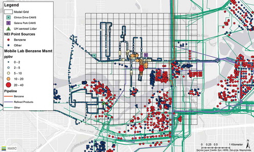
Within Galena Park itself, there are several storage tank farms, as well as port facilities frequented by barges and other ship channel marine traffic, in addition to land-based truck and railroad traffic. There is also an underground pipeline network that transports chemical feedstock and products to and from petrochemical facilities in the area. These emission sources are also shown in Figure 1. The 2011 National Emissions Inventory (NEI) was used to assign initial guess estimates of benzene emissions to each point source unit with a unique Emission Point Number (EPN) in the BEE-TEX study area as a prelude to inverse modeling, with combustion sources assigned a nominal release height of 10 m. An initial conservative estimate of 0.0001 lbs/day of benzene emissions per 200-m segment was assigned to pipelines listed as carrying either benzene or refined product by the Texas Railroad Commission.

Figures 1 and 2 show HARC mobile laboratory measurements of benzene near the Houston Ship Channel in the afternoon and evening of 19 February 2015. Note that the peak measurement of ~37 ppb_v occurs right on top of a segment of the pipeline network in Galena Park carrying refined product, as shown in Figure 1. This indicates that pipeline leaks of benzene were potentially important during the observational episode.

Figure 2. HARC mobile laboratory measurements of benzene on February 19 2015 for Period 1 (afternoon) and Period 2 (evening).

Figure 2 shows that the largest benzene peak measured by the HARC mobile laboratory occurred at 3:27 p.m. local standard time (LST), accompanied by secondary peaks between 3:06 p.m. and 5:14 p.m. LST, which we shall refer to as Period 1 (afternoon). The second largest benzene peak of ~20 ppb_v occurred at 7:12 p.m. LST, also accompanied by lesser peaks between 7:00 p.m. and 8:45 p.m. LST, which we shall refer to as Period 2 (evening). Note that the TCEQ’s short-term (1-hr) human health AMCV for benzene is 180 ppb_v. Background mixing ratios of benzene estimated from the PTR-MS measurements were 0.25 and 0.21 ppb_v for Period 1 and Period 2, respectively. For comparison, the automated gas chromatograph at the Clinton Drive monitoring station near the western edge of Galena Park (see Figure 1) measured late afternoon benzene mixing ratios of around 0.29 ppb_v. We adopted this somewhat higher value as an upwind chemical boundary condition for modeling purposes, as the winds during the time periods of interest were southeasterly, i.e., from the more industrially intensive areas of the ship channel.

Although the HARC mobile laboratory conducted on-board meteorological measurements, these were used mostly to provide instantaneous guidance on plume transport. They were not, however, used for post hoc modeling analyses, as local winds could often be gusty and difficult to extrapolate to other areas in the analysis domain. For more rigorous source attribution analyses, we instead utilized time-averaged data for resultant wind speed, resultant wind direction, and outdoor temperature based on hourly average measurements at the Galena Park CAMS (see Figure 1). These data are shown in Table 1

Table 1. Time-averaged meteorological data based on hourly average measurements at the Galena Park CAMS in the afternoon and evening of February 19, 2015.

Time Period	Resultant Wind Speed (m/sec)	Resultant Wind Direction (°)	Outdoor Temperature (K)
3:00 p.m. to 5:00 p.m. LST	4.36	127	288.2
7:00 p.m. to 9:00 p.m. LST	3.64	127	286.3

To gauge the extent of turbulent vertical mixing, we relied on measurements from an aerosol Lidar operated by the University of Houston (UH) during BEE-TEX. This instrument was located next to the main entrance of the refinery on 97th Street in Manchester across the ship channel from Galena Park (see Figure 1). Boundary layer heights estimated from the aerosol Lidar data were 664 and 619 m for Period 1 and Period 2, respectively.

Meteorological extrapolation and transport parameters

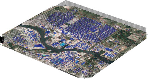
In preparation for source attribution analyses with the HARC air quality model, the wind data of Table 1 were extrapolated throughout an analysis domain indicated by the raster grid in Figure 1, which serves as the air quality model horizontal grid. Note that both the Galena Park CAMS and the aerosol Lidar in Manchester were within this analysis domain. Meteorological data assimilation and extrapolation were performed using the Quick Urban Industrial Complex (QUIC) model developed by Los Alamos National Laboratory (Singh et al., 2008).

The air quality model grid of Figure 1 has a horizontal resolution of 200 m and an equal length and width of 4 km. The QUIC model grid used to extrapolate the wind measurements extends further outward by 100 m on each side of the horizontal domain to enable a mass-consistent Arakawa C-grid to be used for the air quality simulation, and has higher horizontal resolution (5 m) to allow importation of Lidar data for urban morphology, which were obtained from the National Geospatial-Intelligence Agency.

The vertical domain for both the air quality and meteorological grids extends to 300 m above ground level (AGL). The air quality vertical grid has 10 cells, whereas the meteorological grid has 20. Vertical resolution in both grids varies with height and increases toward the surface, with a minimum thickness of 1 m and a maximum thickness of 37 m in the meteorological grid.

Note that the extent of the horizontal domain is equivalent to the size of a single grid box in a typical regional model, so a vertical extent that is approximately half the boundary layer height is not inappropriate for this application given the limited temporal duration of the episodes examined and the lack of convective mixing in the late afternoon and evening. Moreover, plume images from differential absorption Lidar (DIAL) measurements (e.g., Hoyt and Raun, 2015) show that fresh industrial benzene plumes stay well below 300 m at the downwind distances of primary interest to this study.

Wind simulations in the presence of urban built structures were performed using the QUIC model for both Period 1 and Period 2, with the resultant wind data in Table 1 used as input for the anemometer level (10 m AGL) background wind, ignoring the differences in time period length between the simulations and the averaging times of Table 1 (due to the format of the TCEQ-provided data). The background wind was vertically extrapolated using a logarithmic profile with an assumed roughness length of 0.1 m, and an inverse Monin-Obukhov length of 0 m⁻¹ for neutral stability (Period 1) and 0.01 m⁻¹ for nocturnal stable conditions (Period 2). Note that the simulated winds included nonzero vertical velocities due to the urban morphology. Streamlines of the horizontally varying wind at the surface for Period 1 are shown in Figure 3, as an example of the QUIC model output.

Figure 3. Wind streamlines (red arrows) output from the QUIC model for Period 1. The urban morphology derived from Lidar data is also shown.

Because the air quality model converts between volume mixing ratios (ppb_v) and mass concentrations (µg/m³), a vertical extrapolation of the surface temperatures in Table 1 is required. For this purpose, lapse rates of 0.00975 and 0 K/m were assumed for Period 1 and Period 2, respectively.

Finally, boundary layer heights derived from UH aerosol Lidar measurements led to estimated coefficients of vertical diffusion based on the urban boundary layer parameterization of Delle Monache et al. (2009). The horizontal turbulent diffusion coefficient was set at 50 m²/sec as in previous applications of the HARC model. The horizontal and vertical winds simulated by the QUIC model and the estimated vertical and horizontal turbulent diffusion coefficients provided the basis of pollutant transport in the air quality model, with an assumed dry deposition velocity of 0.1 cm/sec for benzene (Lefebre et al., 2004).

Model source attribution and plume reconstruction

The HARC model was used to attribute observed benzene plumes to specific emission points, to quantify benzene emissions averaged over the measurement time period, and to extrapolate benzene plume concentrations in areas beyond the mobile laboratory trajectory based on inferred emissions. Similar applications of the HARC model have been discussed in the context of previous field campaigns involving research-grade measurements, including the Second Texas Air Quality Study (TexAQS II; Olaguer, 2013) and the Study of Houston Atmospheric Radical Precursors (SHARP; Buzcu Guven et al., 2013; Olaguer et al., 2013).

A key input parameter in the application of the 4Dvar technique to micro-scale inverse modeling is the initial estimate of the error covariance for emissions at each pipeline segment or EPN-identified point source unit. This parameter is essentially a measure of the uncertainty of the stochastic emissions at the individual sources. The 4Dvar method iteratively adjusts model parameters such as emissions and their error covariances in order to optimize the agreement between model predictions and ambient concentration observations, as measured by a cost function. However, the initial estimates of the error covariances are arbitrary and can be externally adjusted apart from the 4Dvar method to enhance the optimization of the cost function. Thus, the inverse modeling-inferred emissions are the result of a combination of mathematically automated and heuristic tuning. The values of the initial benzene emission error covariances used to derive the results presented here were 2 × 10⁸ (µg/sec)² and 1 × 10⁸ (µg/sec)² for Period 1 and Period 2, respectively, for all sources. Other important inverse modeling parameters include the PTR-MS measurement error, which was assumed to be 1 ppb_v, and the initial background (initial condition) concentration error covariance, which was set at 100 (µg/m³)².

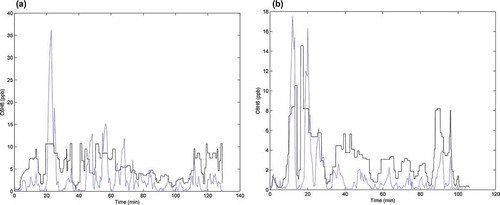
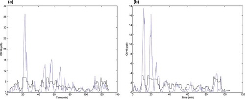
As in previous applications, five forward-adjoint iterations of the model were sufficient for the cost function to converge. Figure 4 compares the simulated benzene volume mixing ratios with ambient measurements along the mobile laboratory trajectory after five model iterations. Note that for Period 1, the model was tuned to agree well with measured secondary peaks at the expense of underestimating the primary peak, whereas the reverse is true for Period 2.

Figure 4. Simulated benzene volume mixing ratios (black line) versus ambient measurements (blue line) along mobile laboratory trajectory for (a) Period 1 (3:06 p.m. to 5:14 p.m. LST) and (b) Period 2 (7:00 p.m. to 8:45 p.m. LST).

We repeated the 4Dvar optimization assuming no pipeline network emissions and the same initial estimates for the emission error covariances. The results of this sensitivity study are displayed in Figure 5. The point source emissions appear to explain much of the observed ambient concentration pattern outside major peaks, but pipeline emissions do appear to be necessary in explaining the larger benzene mixing ratios measured by the HARC mobile laboratory.

Figure 5. Same as in Figure 4, but with no pipeline emissions in the 4Dvar optimization.

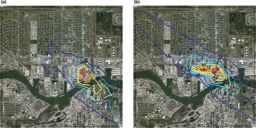
The extrapolated contours of benzene mixing ratio at the end of each time period are presented in Figure 6 for the case with both point source and pipeline emissions. The extrapolated peak concentrations more or less coincide in location for both time periods, although there is an apparent double maximum inferred for the evening. This may reflect the importance of later storage tank emission events, as demonstrated below.

Figure 6. Simulated contours of benzene volume mixing ratio in the analysis domain for (a) Period 1 (3:06 p.m. to 5:14 p.m. LST) and (b) Period 2 (7:00 p.m. to 8:45 p.m. LST) when both point source and pipeline emissions are optimized.

Tables 2 and 3 display inferred emissions from the top 15 emission sources in the 16-km² model domain during Period 1 and Period 2, respectively. Eleven sources are common to both tables, whereas storage tank stack emissions appear to be more important in the evening than in the afternoon. Pipeline emissions are at least partly responsible for the measured peaks in ambient benzene concentration during both observation periods, but there are also important source contributions from marine, railcar, and tank truck loading/unloading facilities.

Table 2. Benzene source attribution results for Period 1 (top 15 sources only).

Emission Point Number (EPN) or Pipeline ID	Average UTMx (m)	Average UTMy (m)	Emissions (kg/hr)
8 pipeline segments with ID 56121–56156	283433.7	3290833	2.97
SD2 (marine loading flare), WTCR (tank truck loading flare)	284029	3290550	2.37
BD2 (marine loading flare)	284205.6	3290463	1.97
TR10 (rail car and tank truck loading flare)	284099	3290509	1.94
29 pipeline segments with ID 59697–61076	284433.7	3290233	1.60
104 pipeline segments with ID 57442–59880	284433.7	3290433	1.37
201 pipeline segments with ID 60905–89418	284633.7	3290033	1.31
81 pipeline segments with ID 59477–60990	284633.7	3290233	1.29
8 pipeline segments with ID 60935–70805	284433.7	3290033	1.28
1 pipeline segment with ID 62374	284833.7	3290033	1.24
3 pipeline segments with ID 56110–56202	283833.7	3290833	1.08
5 pipeline segments with ID 63583–85520	285033.7	3289833	1.08
T187-1, T80-18 (storage tank stacks)	283892.8	3290827	1.06
4 pipeline segments with ID 56101–57129	284033.7	3290833	1.04
2 pipeline segments with ID 56130–56383	283033.7	3290833	1.02

Notes: UTM coordinates are average locations of implicated sources in the same model grid box.

Table 3. Benzene source attribution results for Period 2 (top 15 sources only).

Emission Point Number (EPN) or Pipeline ID	Average UTMx (m)	Average UTMy (m)	Emissions (kg/hr)
3 pipeline segments with ID 56110–56202	283833.7	3290833	0.98
6 pipeline segments with ID 56113–56202	283633.7	3290833	0.81
SD2 (marine loading flare), WTCR (tank truck loading flare)	284029	3290550	0.75
1 pipeline segment with ID 56130	283233.7	3290833	0.63
BD2 (marine loading flare)	284205.6	3290463	0.54
TR10 (rail car and tank truck loading flare)	284099	3290509	0.49
T25-3, T12-5, T12-1, T12-10, T12-3, T25-10, T25-15, T25-14, T25-17, T25-4, T25-6, T25-8, T25-7 (storage tank stacks)	284215.6	3290619	0.46
T187-1, T80-18 (storage tank stacks)	283892.8	3290827	0.43
29 pipeline segments with ID 59697–61076	284433.7	3290233	0.41
T12-24, T12-30, T80-20, T80-19, T12-28, T25-12, T25-13, T25-19, T25-18 (storage tank stacks)	284049.6	3290625	0.41
104 pipeline segments with ID 57442–59880	284433.7	3290433	0.40
4 pipeline segments with ID 56101–57129	284033.7	3290833	0.39
T12-27, T12-25, T12-29 (storage tank stacks), VCU1A&B (thermal oxidizer flare)	284053.7	3290491	0.37
81 pipeline segments with ID 59477–60990	284633.7	3290233	0.36
1 pipeline segment with ID 62374	284833.7	3290033	0.33

Notes: UTM coordinates are average locations of implicated sources in the same model grid box.

We were not able to confirm the presence of railcars in the analysis domain, either visually or after the fact. Railcar activities are proprietary information of commercial shippers. Port of Houston records do show that a tanker and barges had been operating in the afternoon and evening of February 19 2015 at the Kinder Morgan port terminal where the marine loading facilities are located. The tanker was present from 8:52 a.m. to 3:19 p.m. LST, whereas barge operations lasted from 4:23 p.m. to 6:41 p.m. LST.

Table 4 shows total domain emissions of benzene for both point sources and pipelines during Period 1 and Period 2, as well as the relevant 2011 NEI point source estimates. The NEI estimates are comfortably between the inferred Period 1 and Period 2 point source emissions. Pipeline emissions are approximately twice as large as point source emissions for both time periods. Finally, total inferred benzene emissions for the model domain are between 2 and 6 times greater than the corresponding 2011 NEI estimates. The magnitude of the difference between the inferred emissions and the inventory values is roughly consistent with discrepancy factors for industrial volatile organic compound (VOC) emissions estimated using either DIAL (Chambers et al., 2008; Hoyt and Raun, 2015) or the solar occultation flux (SOF) technique (Mellqvist et al., 2010).

Table 4. Total domain emissions of benzene (kg/hr) for point sources and pipelines.

Time Period	Point Sources	Pipelines	Total Emissions
Afternoon	16.43	34.73	51.16
Evening	5.59	10.69	16.29
2011 NEI	8.27	0	8.27

The source attribution results presented here are, of course, subject to uncertainty stemming from a variety of factors. Possibly the largest source of uncertainty is imprecision in the simulation of wind flow. This was discussed in detail by Olaguer et al. (2013), who conducted a sensitivity study of HARC model-inferred refinery emissions of formaldehyde and sulfur dioxide by comparing inverse modeling results based on mobile laboratory data with and without the urban canopy representation. The level of uncertainty found in that study was of the order of 14%. A more precise quantification of source attribution uncertainty will require the comparison of model-inferred emissions with more explicit measurements of individual point source emission rates, such as with the DIAL technique (e.g., Hoyt and Raun, 2015) or tracer release methods (e.g., Allen et al., 2013).

Discussion and conclusion

A possible scenario emerges from the combination of HARC mobile laboratory observations, atmospheric modeling analyses, and direct observation. A tanker and barges were docked and operating at the Kinder Morgan port terminal in Galena Park during the afternoon and evening of 19 February 2015. Coincident with the marine loading/unloading activity were benzene emissions at marine, and possibly railcar and tank truck loading/unloading facilities, and benzene leaks from pipelines transporting refined product during and after the marine loading/unloading operations. In the evening, after the tanker and barges had left the port terminal, storage tank stack and thermal oxidizer flare emissions became prominent. Stack and flare combustion is typically used for emissions control during tank refilling operations.

Although the point source emissions of benzene inferred during the observational episode are in reasonable agreement with 2011 NEI estimates, the significant pipeline emissions of benzene simultaneously inferred from the PTR-MS measurements are twice as large as the point source emissions. The ambient benzene concentrations accompanying the inferred emissions do not appear to be an immediate threat to human health based on the TCEQ’s short-term AMCV, but if emission events associated with port activity are a common occurrence, then it is plausible that the TCEQ long-term AMCV or the EPA IRIS RfC could be exceeded at certain locations away from routine monitoring stations, particularly in the vicinity of pipelines and port facilities. This hypothesis should be examined in greater detail with long-term monitoring at more locations than covered by the TCEQ network in the Houston Ship Channel. For example, the tomographic scanning method demonstrated in the Manchester neighborhood during BEE-TEX could be used to identify local sources and “hot spots” of air toxics without the need to have continuous mobile coverage.

In conclusion, port operations involving petrochemicals may significantly increase emissions of air toxics from the transfer and storage of materials. Pipeline leaks, in particular, can lead to sporadic emissions greater than in emission inventories, resulting in higher ambient concentrations than are sampled by the existing monitoring network. The use of updated methods for ambient monitoring and source attribution in real time should be encouraged as an alternative to expanding the conventional monitoring network. Although these updated methods are admittedly resource-intensive, they can be used in combination with simpler and less expensive techniques (e.g., citizen-based monitoring) to cover a much larger area, especially when the latter are used to trigger more refined investigations in an adaptive manner based on real-time data broadcasts. Moreover, the increasing use of unmanned aerial vehicles (UAVs) and the availability of miniaturized lasers and other instruments offer the possibility of radically increasing both spatial and temporal coverage in the monitoring of industrial facilities.

Acknowledgment

The authors would like to thank the BEE-TEX field study personnel from the University of Houston for giving them access to the aerosol Lidar data used in their modeling analyses. They also thank Dr Joseph P. Pinto of the U.S. Environmental Protection Agency and Dr. Luca delle Monache of the National Center for Atmospheric Research for their thoughtful comments and suggestions.

Funding

BEE-TEX was funded by the Fish and Wildlife Service of the U. S. Department of the Interior through Harris County, Texas.

Additional information

Funding

BEE-TEX was funded by the Fish and Wildlife Service of the U. S. Department of the Interior through Harris County, Texas.

Notes on contributors

Eduardo P. Olaguer

Eduardo P. Olaguer is the program director for Air Quality Science at the Houston Advanced Research Center in The Woodlands, TX.

Matthew H. Erickson

Matthew H. Erickson was until recently a postdoctoral research scientist at the Houston Advanced Research Center in The Woodlands, TX. He is now at the University of Houston.

Asanga Wijesinghe

Asanga Wijesinghe and Bradley S. Neish are research associates at the Houston Advanced Research Center in The Woodlands, TX.

Bradley S. Neish

Asanga Wijesinghe and Bradley S. Neish are research associates at the Houston Advanced Research Center in The Woodlands, TX.

References

- Allen, D.T., V.M. Torres, J. Thomas, D.W. Sullivan, M. Harrison, A. Hendler, S.C. Herndon, C.E. Kolb, M.P. Fraser, A.D. Hill, B.K. Lamb, J. Miskimins, R.H. Sawyer, and J.H. Seinfeld. 2013. Measurements of methane emissions at natural gas production sites in the United States. Proc. Natl. Acad. Sci. U. S. A. 110:17768–17773. doi:10.1073/pnas.1304880110
- Buzcu Guven, B., E.P. Olaguer, S.C. Herndon, C.E. Kolb, W.B. Knighton, and A.E. Cuclis. 2013. Identification of the source of benzene concentrations at Texas City during SHARP using an adjoint neighborhood scale transport model and a receptor model. J. Geophys. Res. Atmos. 118:8023–8031. doi:10.1002/jgrd.50586
- Chambers, A.K., M. Strosher, T. Wootton, J. Moncrieff, and P. McCready. 2008. Direct measurement of fugitive emissions of hydrocarbons from a refinery. J. Air Waste Manage. Assoc. 58:1047–1056. doi:10.3155/1047-3289.58.8.1047
- De Gouw, J., and C. Warneke. 2007. Measurements of volatile organic compounds in the earth’s atmosphere using proton-transfer-reaction mass-spectrometry. Mass Spectrom. Rev. 26:223–257. doi:10.1002/mas.20119
- Delle Monache, L., J. Weil, M. Simpson, and M. Leach. 2009. A new urban boundary layer and dispersion parameterization for an emergency response modeling system: Tests with the joint urban 2003 data set. Atmos. Environ. 43:5807–5821. doi:10.1016/j.atmosenv.2009.07.051
- Hoyt, D., and L.H. Raun. 2015. Measured and estimated benzene and volatile organic compound (VOC) emissions at a major US refinery/chemical plant: Comparison and prioritization. J. Air Waste Manage. Assoc. 65:1020–1031. doi:10.1080/10962247.2015.1058304
- Lefebre, F., K.D. Ridder, N. Lewyckyj, L. Janssen, J. Cornelis, F. Geyskens, and C. Mensik. 2004. Evaluation of AURORA simulated benzene concentrations for the urban area of Antwerp. In Air Pollution Modeling and Its Application XVI, ed. C. Borrego and S. Incecik, 511–520. New York: Springer.
- Mellqvist, J., J. Samuelsson, J. Johansson, C. Rivera, B. Lefer, S. Alvarez, and J. Jolly. 2010. Measurements of industrial emissions of alkenes in Texas using the solar occultation flux method. J. Geophys. Res. 115:D00F17. doi:10.1029/2008JD011682
- Olaguer, E.P. 2011. Adjoint model enhanced plume reconstruction from tomographic remote sensing measurements. Atmos. Environ. 45:6980–6986. doi:10.1016/j.atmosenv.2011.09.020
- Olaguer, E.P. 2012a. The potential near source ozone impacts of upstream oil and gas industry emissions. J. Air Waste Manage. Assoc. 62:966–977. doi:10.1080/10962247.2012.688923
- Olaguer, E.P. 2012b. Near source air quality impacts of large olefin flares. J. Air Waste Manage. Assoc. 62:978–988. doi:10.1080/10962247.2012.693054
- Olaguer, E.P. 2013. Application of an adjoint neighborhood scale chemistry transport model to the attribution of primary formaldehyde at Lynchburg Ferry during TexAQS II. J. Geophys. Res. Atmos. 118:4936–4946. doi:10.1002/jgrd.50406
- Olaguer, E.P., S.C. Herndon, B. Buzcu Guven, C.E. Kolb, M.J. Brown, and A.E. Cuclis. 2013. Attribution of primary formaldehyde and sulfur dioxide at Texas City during SHARP/formaldehyde and olefins from large industrial releases (FLAIR) using an adjoint chemistry transport model. J. Geophys. Res. Atmos. 118:11317–11326. doi:10.1002/jgrd.50794
- Sandu, A., D.N. Daescu, G.R. Carmichael, and T. Chai. 2005. Adjoint sensitivity analysis of regional air quality models. J. Comput. Phys. 204:222–252. doi:10.1016/j.jcp.2004.10.011
- Singh, B., B.S. Hansen, M.J. Brown, and E.R. Pardyjak. 2008. Evaluation of the QUIC-URB fast response urban wind model for a cubical building array and wide building street canyon. Environ. Fluid Mech. 8:281–312. doi:10.1007/s10652-008-9084-5
- Texas Commission on Environmental Quality (TCEQ). 2011. Air Pollutant Watch List Boundary Supplemental Documentation: Benzene in Galena Park. Austin, TX: Texas Commission on Environmental Quality.
- Zou, X., F. Vandenberghe, M. Pondeca, and Y.-H. Kuo. 1997. Introduction to Adjoint Techniques and the MM5 Adjoint Modeling System. National Center for Atmospheric Research, Technical Note, NCAR/TN-435-STR. Boulder, CO: National Center for Atmospheric Research.