Updated methods for assessing the impacts of nearby gas drilling and production on neighborhood air quality and human health

ABSTRACT

An explosive growth in natural gas production within the last decade has fueled concern over the public health impacts of air pollutant emissions from oil and gas sites in the Barnett and Eagle Ford shale regions of Texas. Commonly acknowledged sources of uncertainty are the lack of sustained monitoring of ambient concentrations of pollutants associated with gas mining, poor quantification of their emissions, and inability to correlate health symptoms with specific emission events. These uncertainties are best addressed not by conventional monitoring and modeling technology, but by increasingly available advanced techniques for real-time mobile monitoring, microscale modeling and source attribution, and real-time broadcasting of air quality and human health data over the World Wide Web. The combination of contemporary scientific and social media approaches can be used to develop a strategy to detect and quantify emission events from oil and gas facilities, alert nearby residents of these events, and collect associated human health data, all in real time or near-real time. The various technical elements of this strategy are demonstrated based on the results of past, current, and planned future monitoring studies in the Barnett and Eagle Ford shale regions.

Implications: Resources should not be invested in expanding the conventional air quality monitoring network in the vicinity of oil and gas exploration and production sites. Rather, more contemporary monitoring and data analysis techniques should take the place of older methods to better protect the health of nearby residents and maintain the integrity of the surrounding environment.

Introduction

There has been an explosive growth in natural gas production within the last decade, as horizontal drilling and hydrofracturing technologies have made feasible the large-scale exploitation of unconventional oil and gas resources. This has been especially true in already pollution-challenged cities that sit atop the Barnett Shale of Texas, such as Denton, Fort Worth, and Arlington. In these cities, exploration and production activities increasingly occur in residential neighborhoods, with required setbacks from population receptors of only a few hundred feet in many cases (Fry, 2013).

The explosion of oil and gas activity in the Barnett Shale has increased air emissions of and human exposure to nitrogen oxide (NO_x) and volatile organic compound (VOC) precursors to ozone (O₃, a lung irritant that exacerbates asthma), and hazardous air pollutants (HAPs, compounds with known or suspected toxic health effects) such as benzene and formaldehyde (Armendariz, 2009). VOCs emitted by oil and gas activities are mainly alkanes and aromatics, with some alkenes and oxygenated hydrocarbons (e.g., aldehydes) produced by incomplete combustion in flares, engines, and reboilers. Table 1 lists the most important HAPs emitted by the oil and gas industry, their human health hazards, and Effects Screening Levels (ESLs) developed by the Texas Commission on Environmental Quality (TCEQ) to determine acceptable ambient concentrations. Note that global background levels of VOCs and HAPs, usually stated as volume mixing ratios, are well below 1 part per billion (ppbv) (American Geophysical Union [AGU], 2009).

According to the TCEQ (2015), the annual average concentration of benzene in the Barnett Shale as measured by state-run monitors has remained well below 1 ppbv, despite the growth in local oil and gas activities. However, annual average measurements by the regional monitoring network do not account for localized pollution plumes in the immediate vicinity of oil and gas sites. Such plumes have often been seen with infrared cameras and reported by activists on the Internet, prompting concerns about possible health hazards by local residents. (For example, see: http://www.texassharon.com/2009/11/24/barnett-shale-tceq-videos-show-fugitive-emissions.)

Concern over the health impacts of gas mining in the Barnett Shale has spilled over into the Eagle Ford Shale region in the vicinity of San Antonio, TX, where the number of oil and gas wells could triple to 32,000 between 2013 and 2018 (Alamo Area Council of Governments [AACOG], 2014). In this case, vociferous complaints have been raised in rural towns such as Karnes City regarding the lack of regulatory protection for residents from bad air quality allegedly due to local oil and gas activities within a few miles of their homes (Song et al., 2014). Increasingly, citizens demand accurate information on oil and gas site emissions and their public health consequences, information that remains scarce despite recent scientific attention (Petron et al., 2012; McKenzie et al., 2012, 2104; Adgate et al., 2014; Bunch et al., 2014). Commonly acknowledged sources of uncertainty are the lack of sustained monitoring of ambient concentrations of pollutants associated with gas mining, poor quantification of their emissions, and inability to correlate health symptoms with specific emission events.

Some previous air quality field studies in the Fort Worth metropolitan area have deployed conventional ambient air monitoring methods, such as Summa canisters and dinitrophenylhydrazine (DNPH) cartridges, and/or direct point source sampling of emissions using toxic vapor analyzers, to determine whether or not human health concerns are justified (Barnett Shale Energy Education Council [BSEEC], 2010; ERG, 2011). However, these conventional methods suffer from severe flaws. In the case of ambient air monitoring using U.S. Environmental Protection Agency (EPA) Methods TO-15 and TO-11, flaws include degradation of captured air samples prior to off-line laboratory analysis, poor temporal and spatial coverage, and inability to adjust to variable wind direction. Sampling at the emission point using U.S. EPA Method 21, on the other hand, cannot be applied to combustion sources and may be affected by operator behavior.

Zielinska et al. (2014) attempted a somewhat more sophisticated monitoring study in the Barnett Shale using a mobile laboratory equipped with a portable photo-ionization detector (PID) to measure ambient VOC concentrations in real time at ppb levels. However, the portable PID monitor could not speciate VOCs, so Zielinska et al. (2014) resorted to traditional canister and DNPH cartridge measurements whenever the PID monitor indicated high ambient VOC concentrations. Eapi et al. (2014) also used a mobile laboratory in the Barnett Shale region to conduct real-time ambient air measurements with a commercial cavity ring-down spectrometer (CRDS), which they used to monitor the greenhouse gas, methane. Allen et al. (2013) measured methane emissions at 190 onshore natural gas production sites in the United States, several of them in Texas, using a variety of techniques, including downwind tracer studies using a mobile laboratory equipped with quantum cascade lasers (QCLs). Similarly advanced real-time measurement techniques using either optical methods or chemical ionization–mass spectrometry (CIMS) are increasingly available to measure ozone precursors and air toxics (Olaguer et al., 2014).

The Dallas–Fort Worth (DFW) area (10 counties) is in nonattainment of the federal ozone standard, whereas the San Antonio area (4 counties) is currently designated as in ozone attainment. The TCEQ has recently increased the number of automated gas chromatograph (auto-GC) stations in DFW from 2 to 15 to monitor the growth in hydrocarbon emissions from oil and gas activities and their ozone impacts. However, the TCEQ auto-GC network remains too sparse to reliably detect large transient emission events due to process upsets, maintenance, startups, and shutdowns at oil and gas sites, or even regular plumes emanating from approximately 4000 stationary engines, many rated at thousands of horsepower. Using a microscale air quality model, Olaguer (2012a) demonstrated that flares and engines at natural gas processing and pipeline compression facilities can result in very narrow but nonetheless significant ozone and formaldehyde plumes 2–10 km downwind. Such pollution plumes may impact nearby communities without being detected by the TCEQ monitoring network in the Barnett Shale, and all the more so in the Eagle Ford where there are, thus far, only two auto-GC monitoring stations (Hiller and Tedesco, 2014).

To properly assess the health consequences of oil and gas-related air pollution will require more widespread deployment of new techniques for real-time air quality monitoring and microscale modeling. In addition, the valuable information generated by these technologies can empower local citizens if data can be broadcast in real time over the World Wide Web and made accessible to the public via contemporary mobile devices. Our goal is to demonstrate the application of these new technologies and what they may reveal about oil and gas operational impacts in the context of previous and future studies in the Barnett and Eagle Ford shale regions of Texas, and to show how the combination of scientific and social media approaches may yield previously unavailable information that empowers communities to make decisions regarding human health in neighborhoods where oil and gas activities occur. We have therefore chosen the form of a “notebook” paper to present a couple of pilot studies in the Barnett and Eagle Ford shale regions that support our theme of the feasibility of advanced approaches, specifically those that combine real-time monitoring, data broadcasting, and high-resolution modeling, in assessing the air quality and human health impacts of the oil and gas industry.

Microscale modeling

The first technology we demonstrate is a three-dimensional (3D) microscale Eulerian air quality model that can be used not only in the traditional forward mode, that is, to simulate the pollution concentration field resulting from specified (usually industry-reported) emissions, but also in inverse mode, that is, to infer the location, timing, and quantity of pollutant releases from specific emission points in a facility based on ambient measurements of pollutant concentration. This model, which we refer to as the Houston Advanced Research Center (HARC) model, has been documented and evaluated based on field observations in several publications (Olaguer, 2011, 2012a, 2012b, 2013; Buzcu Guven et al., 2013; Olaguer et al., 2013).

The HARC model is coded in MATLAB and simulates transport by both advection and turbulent diffusion. It is driven by winds from the Quick Urban and Industrial Complex (QUIC) microscale meteorological model (Singh et al., 2008) based on 3D urban morphological data from Lidar observations, or from industrial permits as in the present case. The continuous adjoint of the transport model required for inverse estimation of emissions is simply advection by the reverse of the forward model wind, whereas diffusion is self-adjoint. While the HARC model can simulate air chemistry due to emissions of reactive species, the specific model experiment described in this particular section does not require this capability.

The objective of our model experiment is to infer process-specific emissions of the air toxic formaldehyde (HCHO) from a pipeline compressor station in the Barnett Shale based on ambient air observations immediately adjacent to the station, rather than on measurements conducted further away from the facility. HCHO has a typical atmospheric lifetime of about 3 hr, whereas the modeling experiment concerns a 1-hr emissions scenario and associated fenceline concentrations. This enables us not only to ignore the details of the atmospheric degradation of HCHO, but also to use much higher horizontal resolution (10 m) within a smaller domain (400 m × 400 m horizontal; 150 m vertical with 10 variably spaced levels) than would otherwise be required. The specific chemical observations we use to drive the inverse model are in this case not advanced real-time (~1 sec time response) measurements, but conventional DNPH cartridge measurements performed by Titan Engineering during a study conducted by the Barnett Shale Energy Education Council (BSEEC) in Fort Worth, TX. Details of the sampling scheme are provided in the BSEEC (2010) report.

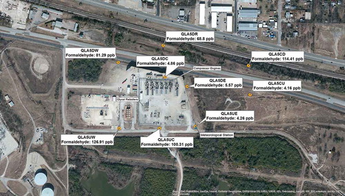
Figure 1 depicts 1-hr average measurements of HCHO outside the pipeline compressor station in the afternoon of June 11, 2010, during the BSEEC study. As a conservative indication of public health concern, the TCEQ stipulates a short-term (1-hr) ESL for ambient HCHO of 12 ppb. Note, however, the very large ambient HCHO concentrations approaching or even surpassing 100 ppb around the facility, mixed with concentrations near or below 4 ppb (a more typical concentration level observed at oil and gas sites during the BSEEC study). The BSEEC (2010) study report attributed the high concentrations either to nearby mobile sources or to a more distant upwind source to the south of the pipeline compression station. The observed HCHO concentrations are unlikely due to automotive emissions, as documented short-term near-road concentrations in the United States are at most ~17 ppb (Health Effects Institute [HEI], 2007). The patchiness of the ambient concentration field also argues against a more distant source, and instead points to a possible emission event at the compressor station in the presence of a nonuniform wind pattern caused by the sound barrier and other built structures at the compressor station. Our hypothesis also better explains the observed HCHO concentration pattern than field sampling problems involving multiple DNPH cartridges, even if validation (duplicate) data were missing due to a pump failure, as indicated in the BSEEC (2010) report. We demonstrate the viability of our hypothesis via an explicit simulation of the wind field, informed by whatever meteorological data was collected at the relevant site during the BSEEC study.

Figure 1. One-hour measurements of HCHO (indicated in red) during the BSEEC (2010) study at a pipeline compressor station in the Barnett Shale in the afternoon of June 11, 2010. Note that the top of the figure points northward.

A Met One AutoMet weather monitoring system with a 3-cup anemometer and a balanced anodized aluminum vane was set up at the southeast corner of the compressor station (see Figure 1) during the BSEEC (2010) study. Wind measurements were reported with an averaging time of 15 min, and are shown in Table 2 for the time period of interest. A dispersion modeling appendix to the study report indicates that wind observations were applied at a standard anemometer height of 10 m.

Table 1. Most important hazardous air pollutants (HAPs) emitted by the oil and gas industry and their effects screening level (ESL) values as determined by the state of Texas.

		Short-term	Long-term
HAP	Health hazard	ESL (1-hr)	ESL (24-hr)
Benzene	Cancer	54 ppb	1.4 ppb
Toluene	Respiratory symptoms	920 ppb	330 ppb
	Neural symptoms
C2-Benzenes	Respiratory symptoms	58-380 ppb	42 ppb
	Neural symptoms
n-Hexane	Neural symptoms	1500 ppb	57 ppb
Formaldehyde	Cancer	12 ppb	4.5 ppb (cancer)
	Respiratory symptoms		2.7 ppb (noncancer)

Table 2. Measurements of wind speed and direction in the afternoon of June 11, 2010, at the pipeline compressor station during the BSEEC (2010) study.

Local time	Wind speed (mph)	Wind direction (deg)
14:15	8.2	181.7
14:30	8.0	178.9
14:45	8.2	180.0
15:00	7.7	177.5
15:15	8.2	173.8

To simulate the wind flow in the vicinity of the compressor station, we constructed a 3D digital model of the facility and its surroundings at 5 m horizontal resolution based on industrial permit data, aerial photographs, and specifications from equipment manufacturers. The height of the compressor engines and other major built structures was assumed to be 3 m.

The finer resolution (5 m) and somewhat wider domain (405 m × 405 m) of the meteorological grid allowed us to construct a mass-consistent Arakawa C-grid for the HARC model simulation, as previously described by Olaguer et al. (2013). Based on the measurements of Table 2, we postulated a background southerly flow, with a wind speed of 3.58 m/sec at a height of 10 m above ground level. The QUIC model then computed the mass-consistent flow around obstacles throughout the entire model domain based on the digital morphological model, which included a representation of the tree canopy with an attenuation coefficient of 2.74. Values for the roughness length and inverse Monin–Obukhov length assumed for the QUIC model run were 0.1 m and −0.01 m⁻¹, respectively. The HARC model, driven by winds from the QUIC model, then minimized a cost function related to the difference between the concentration predictions of the forward model and the HCHO observations to infer emissions from each unit in the facility, using permit data as first-guess emission estimates. The underlying technique is known as four-dimensional (4D) variational data assimilation, the HARC model implementation of which was discussed in detail by Olaguer (2013) and Olaguer et al. (2013).

Figure 2 shows the wind flow around the facility simulated by the QUIC urban wind model, as well as air concentrations of HCHO inferred by the HARC model based on inverse model-optimized emissions from the facility’s compressor engines and glycol reboilers. For convenience, these results are also presented in Table 3 along with the corresponding measured concentrations. The results of the HARC model point to a possible emission event at the glycol reboilers, with HCHO event emissions as high as 6 kg/hr averaged over 1 hr, perhaps due to equipment malfunction.

Table 3. Model-inferred HCHO concentrations vs. measurements from BSEEC (2010) study.

Measurement site	Measured concentration	Simulated concentration
QLA5DW	81.3 ppb	69.2 ppb
QLA5DR	68.8 ppb	44.1 ppb
QLA5DC	4.86 ppb	80.3 ppb
QLA5DE	5.57 ppb	16.8 ppb
QLA5CD	114.4 ppb	1.48 ppb
QLA5CU	4.16 ppb	1.42 ppb
QLA5UE	4.26 ppb	4.01 ppb
QLA5UC	100.3 ppb	88.1 ppb
QLA5UW	126.9 ppb	62.3 ppb

Figure 2. Airflow (blue streamlines) near the surface at the oil and gas site of Figure 1 in the afternoon of June 11, 2010, as simulated by the QUIC urban wind model assuming a southerly background wind. Also shown are 1-hr average ambient concentrations of HCHO (indicated in red) simulated by the HARC air quality model based on assimilated measurements from the BSEEC (2010) study.

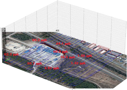
The normalized root-mean-square deviation between the DNPH measurements of HCHO and the simulated ambient concentrations based on the inferred emissions is 14%. The greatest deviations are between the sound barrier and the compressor engines, and also east of the sound barrier. The discrepancies may be due to the imperfect rendering of nearly two-dimensional (2D) objects (such as the sound barrier) by the QUIC modeling software, as well as unrepresented fanning action by the compressor engines. The high HCHO concentrations simulated by the HARC model at the upwind edge of the facility are consistent with the observations, and are due to air counterflow caused by the sound barrier and other structures at the compressor station.

The facility permit acknowledges only very limited HCHO emissions (<0.01 tons/yr) from the glycol reboilers implicated by the inverse modeling, and in practice HAP emissions from this type of unit are only estimated for benzene, toluene, ethylbenzene, and xylenes (BTEX) using the Gas Technology Institute’s GLYCalc model. Our simulation results illustrate how an advanced microscale model can indicate the existence of previously unsuspected emission events at oil and gas facilities, and quantify ambient exposure to HAPs released to surrounding neighborhoods during these events. We caution, however, that our modeling exercise is merely illustrative, and that better and more extended measurements than possible with the DNPH cartridge technique may be needed to more definitively identify and quantify potentially harmful emission events. In the next section, we demonstrate how this may be done using a specific real-time monitoring technology.

Real-time air quality monitoring

In 2014, HARC conducted a limited study of oil and gas emissions and related air quality impacts in the Eagle Ford Shale. To provide real-time monitoring for the Eagle Ford study, a Ford E-350 passenger van was outfitted with a number of scientific instruments (see Figure 3). To ensure adequate power for these instruments, the van’s electrical system was first upgraded to a 225-A alternator. The power created by the larger alternator was split between the engine battery and a pair of deep cycle auxiliary batteries using a ProSplit Battery Isolator, number PSR182. A ProWatt Square Wave 2000 Inverter was then connected to the auxiliary batteries to continuously deliver 13 A at 120 V AC. For stationary applications, an Auto Transfer Switch enabled access to external 120 V AC power, and a 120-V AC air conditioner cooled the van when the normal dual air conditioning system was not in use.

Figure 3. (Left) Mobile Acquisition of Real-Time Concentrations (MARC) vehicle. (Right) Position of anemometer and sample inlet mounted on top of MARC.

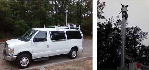
An ultrasonic anemometer (R. M. Young model 85000) was used to measure wind speed and direction. The anemometer was mounted on a 3-ft pole on top of the van to enable these measurements to be conducted approximately 13 ft above ground level. A temperature and relative humidity probe (R.M. Young model 41382) was also mounted on top of the van. A global positioning system (GPS; Garmin GPS 19x HVS) was mounted at the center of the roof to record the van’s position.

An Ionicon quadrupole proton transfer reaction mass spectrometer (PTR-MS) was mounted inside the van to measure BTEX compounds. The back seats of the van were removed and the PTR-MS was secured to the floor using wire-rope isolators. This precaution was necessary to ensure the stability of the turbo molecular pumps in the PTR-MS, which are sensitive to mechanical shocks. In addition, the PTR-MS was backed up with an uninterruptible power supply (UPS) to enable switching between external power and van power without the need to shut down the instrument. A sample line (Swagelok, 1/4-inch PFA) from the PTR-MS to the top of the van allowed air to be sampled near the anemometer to ensure that the wind measurements are representative of the air sample. A Gast vacuum compressor pump was used to pull air through the sample line at a rate of 10 slpm to minimize residence time within the sample line and ensure fast response.

The PTR-MS is capable of measuring a large variety of VOCs in real time at the sacrifice of precise speciation in some cases. A detailed description of the PTR-MS operation is provided by De Gouw and Warneke (2007). Sampled species are ionized via a proton transfer reaction with the hydronium ion (H₃O⁺). Compounds are identified by their mass to charge ratio (m/z), which is typically equal to the molecular weight (MW) of the compound plus one (MW + 1). For example, the MW of benzene is 78 and will respond at m/z = 79 within the PTR-MS. This method allows for fast measurement, even multiple times per second if desired, with limits of detection typically under 1 ppbv.

A drawback of the PTR-MS technique as currently implemented is an inability to distinguish isomers (although newer versions of the Ionicon instrument are now available that remedy this problem with the aid of a fast GC column). For example, ethylbenzene, o-xylene, p-xylene, and m-xylene all contribute to the response at m/z = 107. This is often not an issue, since the response at m/z = 107 is simply attributed to the response of all C2-benzenes. Despite its drawbacks, the PTR-MS is a fast, reliable method for mobile monitoring of VOCs.

There are two modes in which the PTR-MS is operated: plume tracking and plume characterization. For plume tracking, only a few key ions are measured at a fast rate to ensure that the plume can be monitored while the van is in motion. For example, if the BTEX compounds are of primary interest, the PTR-MS would only need to measure at m/z = 79 (benzene), m/z = 93 (toluene), and m/z = 107 (xylenes and ethylbenzene). This would result in a data point for each species every 5 sec (response time), which is more than sufficient for tracking a plume. Multiple passes are often required to measure background levels outside the plume as well as the level of pollutants in the plume. Figure 4 shows the benzene mixing ratios observed by MARC while monitoring a plume resulting from a large flare associated with natural gas production during the Eagle Ford study. The gaps in the data correspond to when the PTR-MS was in the second mode of operation (plume characterization).

Figure 4. Example of plume tracking with MARC as it passes periodically through the plume of a large flare. The gaps are associated with periods where numerous barscans were performed to aid in identifying other potential hazardous pollutant emissions.

In the second or “barscan” mode, the PTR-MS measures ions within a wide range of m/z values (e.g., 21 to 140). This mode is inherently slower (~1 min per scan), but adds valuable information on plume composition. This data can be drawn upon to infer relationships between species that are not monitored when operating in the first mode, and provides the opportunity to determine whether there are other ions that should be monitored during plume tracking. In many cases, however, fragmentation of the parent compound results in interferences at lower m/z values (e.g., for light alkanes). These interferences are minimized to the extent possible by controlling the kinetic energy of ions moving through the reaction chamber as measured in Townsends (Td). Figure 5 shows an example of a barscan obtained during the Eagle Ford study, during which the PTR-MS was operated at 120 Td. Shown is the raw signal observed by the PTR-MS, which can be translated into a compound-specific mixing ratio by subtracting the background signal and applying the sensitivity generated from calibration.

Figure 5. Barscan of an emission plume related to oil and gas production operations.

Calibrations for the PTR-MS are performed by sub-sampling from a flow of dynamically diluted certified calibration standard. A low flow of calibration gas is diluted by a high flow of zero air to generate a desired mixing ratio. For example, 100 sccm flow of 1 ppmv of benzene diluted by 2000 slpm of zero air (hydrocarbon free) would result in a mixing ratio of ~48 ppbv of benzene. The zero air was generated by running ambient air through a hydrocarbon trap (Restek, Nickel-Plated Brass). The PTR-MS subsamples from the diluted gas flow and the response is observed (signal subtracted by the known background signal). This response is linearly proportional to the mixing ratio of the species and is used to convert PTR-MS signals to mixing ratios during normal operation.

The PTR-MS was calibrated periodically using a standard BTEX cylinder (Matheson) with an accuracy of 5%. When the signal was stable during calibrations, the standard deviation of the signal was less than 6%. The detection limits of benzene, toluene, and C2-benzenes were estimated at 0.7, 1.0, and 1.25 ppbv respectively. The PTR-MS error assumed for the purpose of inverse modeling was 1 ppbv.

Water vapor can complicate the interpretation of PTR-MS data by causing unwanted reactions in the reaction chamber, particularly for species with a proton affinity similar to that of water. To increase the sensitivity of the PTR-MS for such species, a dehumidifier was installed to lower the water vapor content of sampled air. A simple schematic of the drying system is shown in Figure 6. The dehumidifier utilized a Nafion tube (MD-070-12P-4) from Perma-Pure. The Nafion tube consists of a small tube made of a selectively permeable membrane within a larger tube. The permeable membrane is large enough to allow water to pass through while retaining larger species. Air is flowed through a Drierite tube to remove any water vapor prior to entering the outer tube. This means that the small tube that the sample flows through is surrounded by dry air. The water vapor constantly permeates through the wall in reaching equilibrium. This results in the sample air becoming increasingly dry as it travels through the Nafion tube. The drying is more effective if the outer tube dry air flows in the opposite direction as the sample air, thus increasing the exposure of sample air to dry air.

Figure 6. Diagram of dehumidifier system.

All of the mobile laboratory data were recorded through a custom-built LabView program. The wind speed and direction, temperature, relative humidity, and GPS location were recorded at 1 data point per second. The cycle time of the PTR-MS can vary depending on the number of ions observed, but was typically kept below 10 sec per data point during mobile operations.

Initial inspections in the field were conducted to ensure proper data file identification, screen the data, identify unusual events, and perform instrument checks. Samples were flagged when significant deviations occurred. All data were then transferred and archived to an off-site database for more intensive quality assurance after the field campaign. The next section discusses how the mobile lab data were broadcast in real time, in addition to being automatically archived, to allow remote command and control of mobile lab operations.

Real-time data broadcasting

Real-time or near-real-time data broadcasting from a mobile laboratory out in the field presents multiple challenges, including network connectivity, and data storage, access, and visualization. To overcome these challenges a variety of technologies, many of them representing only recently available technological advances (such as WebSockets) were employed.

MARC was equipped with a Verizon MiFi or mobile hotspot, to provide the onboard computer with Internet connectivity. Using custom-coded LabView software, the onboard computer formatted and pushed the readings from the various MARC instruments to a Cloud database via MiFi. Due to the remote location of the site, network latency, and the duration of PTR-MS measurements, real-time broadcast resolution was ~6 sec. Further code was written into the program to handle times when no Internet connection was available by locally storing all data at a high temporal resolution (~1 sec), and to upload these data when the connection came back online. The Cloud database was a spatially enabled PostgreSQL + PostGIS database hosted on an Amazon Web Services instance, which was chosen for its reliability, security, and accessibility.

Using ArcGIS for Server and GeoEvent Processor, the database was monitored in real time for updates from the mobile laboratory and, leveraging HTML5 WebSocket technology, securely displayed in a Javascript-based Web-mapping application to display the location of the van on a map, as well as the readings of the various instruments in tables in charts in near-real time for live monitoring in a Web browser by the researchers both in the van and back at home base. A purely hypothetical example of a Web browser screenshot is shown in Figure 7.

Figure 7. Hypothetical Web browser screenshot of the MARC real-time data broadcasting system. The actual site of the experiment in the Eagle Ford Shale cannot be shown due to a nondisclosure agreement.

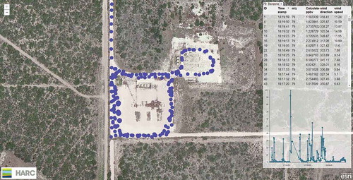
One of the advantages of the MARC data broadcasting system is that it facilitates adaptive monitoring of emission events. The mobile laboratory can be directed very quickly toward critical areas in the vicinity of an industrial facility so that the emission plume can be accurately mapped in preparation for source attribution with the HARC model.

Assessing health impacts based on concentration thresholds

The HARC study in the Eagle Ford Shale was intended to provide data that would enable decisions to be made with regard to human health. A prerequisite to this desired outcome was the quantification of any large emissions from oil and gas facilities located near sensitive receptors. Because the study site and the identity of its proprietor were subjected to a nondisclosure agreement, we cannot show detailed information that would enable readers to deduce the location of the experiment. We can state, however, that the main emission events of interest occurred at a natural gas production facility, for which a detailed digital model was built based on equipment manufacturer data and photographs taken from an unmanned aerial vehicle. All distinct emission points in the facility permit were included in the source attribution, including loading and unloading facilities, storage tanks, separators, glycol reboilers, heater treaters, turbines, compressor engines, and flares. The effective release heights for flare emissions were estimated based on photographs of operating flares. The successful application of the HARC model to the horizontal and vertical dispersion of flare and other combustion plumes has already been demonstrated by Olaguer et al. (2013), including the comparison with airborne measurements of simulated concentrations of reactive products of incomplete combustion, such as formaldehyde, as well as relatively passive tracers such as sulfur dioxide.

Figure 8 shows the MARC trajectory around the production facility and the spatial distribution of benzene measurements corresponding to Figure 4. Based on inverse modeling with a high (20 m horizontal) resolution grid covering the production facility and its immediate vicinity (700 m × 700 m), the large benzene plume of Figures 4 and 8 was determined to be the result of a flare emission of ~28 kg/hr of benzene averaged roughly over an hour. (Note that the combustion plume was plainly visible to mobile lab operators.) This was an order of magnitude greater than routine flare emissions observed at the same facility on other days, and many times larger than emissions attributed by the inverse model to other types of equipment. The inferred emissions for the entire production facility were used as input for a forward model run over a larger domain (4000 m × 4000 m) with coarser horizontal resolution (200 m) than for the inverse model run, so that the ambient concentration of benzene and other species of interest at two sensitive receptors could be assessed. These receptors were residential and/or work areas at which exposure to HAPs was an identified concern of the property owner.

Figure 8. Mobile lab trajectory and corresponding benzene measurements at a natural gas production facility in the Eagle Ford Shale on the day a major flare was observed to be in operation.

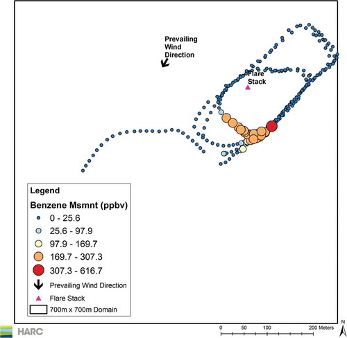
For both the inverse and forward model runs, an average background wind vector of 3.3 m/sec from 30.5° (NNE) was assumed based on mobile laboratory meteorological observations during the episode. Temporal variability of the background wind was not accounted for to avoid complications associated with extrapolating local isolated wind gusts beyond the mobile laboratory location, although spatial variability in the vicinity of built structures near the flare was accounted for by the QUIC wind model. Background concentrations of modeled species were set at the lowest values measured by the PTR-MS. The boundary layer height was assumed to be 1 km during the late afternoon in which the episode occurred.

Figure 9 shows the structure of the flare plume after 2 hr of assumed constant emission in relation to the two receptors, which are located around 3 km away from the flare. Fortunately, the wind was not blowing directly at these receptors, so that an ambient concentration of benzene well below 1 ppbv (18 pptv) was inferred at the two receptor sites (which are close enough to share the same computed grid concentration).

Figure 9. Isopleths of the surface concentration of benzene after 2 hr of flare emission inferred from MARC observations during the Eagle Ford study. Markers denote sensitive receptors.

In addition to the historical episode of the MARC observations, a hypothetical worst-case scenario was considered in which the wind was directly aimed at the two receptors, and the emission scenario was assumed to occur at night to allow for compression of the flare plume by a lower boundary-layer height of 300 m. The results of the worst case scenario are illustrated in Figure 10. Note the significant increase in ambient concentration at the receptors to about 7.3 ppbv benzene. By comparison, the TCEQ’s short-term ESL for benzene is 54 ppbv, so that the worst-case scenario does not exceed the threshold for concern over short-term health impacts by TCEQ standards. Based on normal wind variability, and even considering that the nocturnal mixing height could be as low as 100 m, it is also unlikely that cumulative exposure to large flares may lead to annual average ambient concentrations of benzene at the receptors in question in excess of the TCEQ’s long-term ESL for benzene of 1.4 ppbv. Similar conclusions hold for toluene and C2-benzenes, which were also measured by the PTR-MS during the Eagle Ford study. For these reactive compounds, daytime atmospheric chemistry over the expanded domain was accounted for in the forward model simulation.

Figure 10. Same as in Figure 8, but for the worst-case scenario.

Note that the U.S. EPA Integrated Risk Information System (IRIS) reference concentration (RfC) for chronic inhalation of benzene is 30 µg/m³, or about 9 ppbv. The corresponding chronic inhalation RfCs for toluene, ethylbenzene, and xylenes are approximately 1329 ppbv, 231 ppbv, and 23 ppbv, respectively. We should also bear in mind that real exposures involve mixtures of compounds, about which there is as yet insufficient risk information.

Discussion

The results of the Eagle Ford Shale study just presented do not eliminate concern over possible health effects of oil and gas site emissions, as sensitive receptors can exist closer to flares and other major oil and gas production facilities than those considered here, especially given the low setback distances allowed by Texas municipalities. For example, the large ambient concentrations (~200 ppbv of benzene) in the immediate vicinity of the flare may pose health hazards to oil and gas site workers, especially if there are repeated exposures to such high concentrations over a long period of time. Moreover, other species beyond those measured by the PTR-MS may have emissions greater than benzene or lower threshold levels of concern.

The ground-based mobile monitoring strategy that we advocate has some limitations. For example, road access in rural areas may make it difficult to simultaneously characterize background conditions and pollution plumes emitted by oil and gas facilities. Moreover, the distances between the mobile measurement platform and the emitting sources may limit source attribution and quantification to larger emission events, as opposed to smaller emissions such as routine leaks. Lastly, the limited availability of the measurement platform beyond a few weeks at a time makes it difficult to generate comprehensive statistics on emissions, although it may make it possible to observe a few random emission events.

One way to increase the usefulness of the technologies presented here is to couple advanced scientific measurements and modeling capabilities with social media via Web and mobile device applications that allow for the reporting of human health symptoms in real time. This would enable MARC to alert residents of affected neighborhoods to potential adverse exposures, respond adaptively to reported symptoms, and increase the amount of data that can be used to determine whether or not there is any credible link between oil and gas activities and human health. Symptoms reported via social media in real time can help identify neighborhoods in which emission events may be occurring. Once alerted, MARC operators can quickly obtain biomonitoring (e.g., urine and breath) samples from local residents while emissions are ongoing. For example, human breath samples collected in Tedlar bags can be immediately analyzed with a PTR-MS (Winkler et al., 2013). Biomonitoring results can then be correlated with ambient pollution concentrations measured by MARC and the corresponding emissions inferred from them.

The combination of real-time mobile monitoring, microscale modeling, and human health information makes possible a new generation of public health studies with sufficient analytical power to allow more definitive conclusions to be drawn regarding the impacts of oil and gas activities on surrounding communities. We are already in the process of proposing such studies in Texas shale communities to government and private funding agencies.

Acknowledgments

The authors thank Kim Feil of Arlington, TX, for her assistance in securing industrial permit information for the modeling of the Barnett Shale pipeline compressor station.

Funding

The field study in the Eagle Ford Shale was funded by a private landowner who, while concerned about the possible air quality and health impacts of oil and gas facilities on his estate, insisted on anonymity, so that a nondisclosure agreement prevents us from revealing information sufficient to identify or locate the experimental site.

Additional information

Funding

The field study in the Eagle Ford Shale was funded by a private landowner who, while concerned about the possible air quality and health impacts of oil and gas facilities on his estate, insisted on anonymity, so that a nondisclosure agreement prevents us from revealing information sufficient to identify or locate the experimental site.

Notes on contributors

Eduardo P. Olaguer

Eduardo P. Olaguer is the program director for Air Quality Science at the Houston Advanced Research Center in The Woodlands, TX.

Matthew Erickson

Matthew Erickson was until recently a postdoctoral research scientist at the Houston Advanced Research Center in The Woodlands, TX. He is now at the University of Houston.

Asanga Wijesinghe

Asanga Wijesinghe and Brad Neish are research associates at the Houston Advanced Research Center in The Woodlands, TX.

Jeff Williams

Jeff Williams is the information technology program manager at the Houston Advanced Research Center in The Woodlands, TX.

John Colvin

John Colvin is a research scientist at the Houston Advanced Research Center in The Woodlands, TX.

References

- Adgate, J.L., B.D. Goldstein, and L.M. McKenzie. 2014. Potential public health hazards, exposures and health effects from unconventional natural gas development. Environ. Sci. Technol. 48:8307–20. doi:10.1021/es404621d
- Alamo Area Council of Governments. 2014. Oil and Gas Emission Inventory, Eagle Ford Shale. Technical report 582-11-11219, San Antonio, TX.
- Allen, D.T., V.M. Torres, J. Thomas, D.W. Sullivan, M. Harrison, A. Hendler, S.C. Herndon, C.E. Kolb, M.P. Fraser, A.D. Hill, B.K. Lamb, J. Miskimins, R.H. Sawyer, and J.H. Seinfeld. 2013. Measurements of methane emissions at natural gas production sites in the United States. Proc. Natl. Acad. Sci. USA 110:17768–73. doi:10.1073/pnas.1304880110
- American Geophysical Union. 2009. Volatile organic compounds in the global atmosphere. Eos 90:513–14.
- Armendariz, A. 2009. Emissions From Natural Gas Production in the Barnett Shale Area and Opportunities for Cost-Effective Improvements. Austin, TX: Environmental Defense Fund.
- Barnett Shale Energy Education Council. 2010. Ambient Air Quality Study: Natural Gas Sites, Cities of Fort Worth and Arlington, Texas. Fort Worth, TX: Titan Engineering.
- Bunch, A.G., C.S. Perry, L. Abraham, D.S. Wikoff, J.A. Tachovsky, J.G. Hixon, J.D. Urban, M.A. Harris, and L.C. Haws. 2014. Evaluation of impact of shale gas operations in the Barnett Shale region on volatile organic compounds in air and potential human health risks. Sci. Total Environ. 468–69:832–42. doi:10.1016/j.scitotenv.2013.08.080
- Buzcu Guven, B., E.P. Olaguer, S.C. Herndon, C.E. Kolb, W.B. Knighton, and A.E. Cuclis. 2013. Identification of the source of benzene concentrations at Texas City during SHARP using an adjoint neighborhood scale transport model and a receptor model. J. Geophys. Res. Atmos. 118:8023–31. doi:10.1002/jgrd.50586
- De Gouw, J., and C. Warneke. 2007. Measurements of volatile organic compounds in the earth’s atmosphere using proton-transfer-reaction mass-spectrometry. Mass. Spec. Rev. 26:223–57. doi:10.1002/mas.20119
- Eapi, G.R., M.S. Sabnis, and M.L. Sattler. 2014. Mobile measurement of methane and hydrogen sulfide at natural gas production site fence lines in the Texas Barnett Shale. J. Air Waste Manage. Assoc. 64:927–44. doi:10.1080/10962247.2014.907098
- ERG. 2013. City of Fort Worth Natural Gas Air Quality Study. Fort Worth, TX: ERG.
- Fry, M. 2013. Urban gas drilling and distance ordinances in the Texas Barnett Shale. Energy Policy 62:79–89. doi:10.1016/j.enpol.2013.07.107
- Health Effects Institute. 2007. Mobile-Source Air Toxics: A Critical Review of the Literature on Exposure and Health Effects. Special report 16. Boston, MA: HEI.
- Hiller, J., and J. Tedesco. 2014. A new pollution monitor planned, but gaps remain in the Eagle Ford. San Antonio Express-News, October 24. http://www.expressnews.com/business/eagle-ford-energy/article/A-new-pollution-monitor-planned-but-gaps-remain-5846397.php (accessed December 28, 2015).
- McKenzie, L.M., R.Z. Witter, L.S. Newman, and J.L. Adgate. 2012. Human health risk assessment of air emissions from development of unconventional natural gas resources. Sci. Total Environ. 424:79–87. doi:10.1016/j.scitotenv.2012.02.018
- McKenzie, L.M., R. Guo, R.Z. Witter, D.A. Savitz, L.S. Newman, and J.L. Adgate. 2014. Birth outcomes and maternal residential proximity to natural gas development in rural Colorado. Environ. Health Perspect. 122. doi:10.1289/ehp.1306722
- Olaguer, E.P. 2011. Adjoint model enhanced plume reconstruction from tomographic remote sensing measurements. Atmos. Environ. 45:6980–86. doi:10.1016/j.atmosenv.2011.09.020
- Olaguer, E.P. 2012a. The potential near source ozone impacts of upstream oil and gas industry emissions. J. Air Waste Management Assoc. 62:966–77. doi:10.1080/10962247.2012.688923
- Olaguer, E.P. 2012b. Near source air quality impacts of large olefin flares. J. Air Waste Management Assoc. 62:978–88. doi:10.1080/10962247.2012.693054
- Olaguer, E.P. 2013. Application of an adjoint neighborhood scale chemistry transport model to the attribution of primary formaldehyde at Lynchburg Ferry during TexAQS II. J. Geophys. Res. Atmos. 118:4936–46. doi:10.1002/jgrd.50406
- Olaguer, E.P., S.C. Herndon, B. Buzcu Guven, C.E. Kolb, M.J. Brown, and A.E. Cuclis. 2013. Attribution of primary formaldehyde and sulfur dioxide at Texas City during SHARP/ formaldehyde and olefins from large industrial releases (FLAIR) using an adjoint chemistry transport model. J. Geophys. Res. Atmos. 118:11317–126. doi:10.1002/jgrd.50794
- Olaguer, E.P., C.E. Kolb, B. Lefer, B. Rappenglück, R. Zhang, and J.P. Pinto. 2014, Overview of the SHARP campaign: Motivation, design, and major outcomes. J. Geophys. Res. Atmos. 119:2597–610. doi:10.1002/2013JD019730
- Petron, G., G. Frost, B.R. Miller, A.I., Hirsch, S.A. Montzka, A. Karion, M. Trainer, C. Sweeney, A.E. Andrews, L. Miller, J. Kofler, A. Bar-Ilan, E.J. Dlugokencky, L. Patrick, C.T. Moore, T.B. Ryerson, C. Siso, W. Kolodzey, P.M. Lang, T. Conway, P. Novelli, K. Masarie, B. Hall, D. Guenther, D. Kitzis, J. Miller, D. Welsh, D. Wolfe, W. Neff, and P. Tans. 2012. Hydrocarbon emissions characterization in the Colorado Front Range: A pilot study. J. Geophys. Res. Atmos. 117. doi:10.1029/2011JD016360
- Singh, B., B.S. Hansen, M.J. Brown, and E.R. Pardyjak. 2008. Evaluation of the QUIC-URB fast response urban wind model for a cubical building array and wide building street canyon. Environ. Fluid Mech. 8:281–312. doi:10.1007/s10652-008-9084-5
- Song, L., J. Morris, and D. Hasemyer. 2014. Fracking boom spews toxic air emissions on Texas residents. Inside Climate News, February 18. http://insideclimatenews.org/news/20140218/fracking-boom-spews-toxic-air-emissions-texas-residents (accessed December 28, 2015).
- Texas Commission on Environmental Quality. 2015. Air Quality Successes–Air Toxics. http://www.tceq.state.tx.us/airquality/airsuccess/air-success-toxics (accessed April 2, 2015).
- Winkler, K., J. Herbig, and I. Kohl. 2013. Real-time metabolic monitoring with proton transfer reaction mass spectrometry. J. Breath Res. 7:036006. doi:10.1088/1752-7155/7/3/036006
- Zielinska, B.K., D.E. Campbell, and V. Samburova. 2014. Impact of emissions from natural gas production facilities on ambient air quality in the Barnett Shale area: A pilot study, J. Air Waste Manage. Assoc. 64:1369–83. doi:10.1080/10962247.2014.954735