Evaluation of low wind modeling approaches for two tall-stack databases

Abstract

The performance of the AERMOD air dispersion model under low wind speed conditions, especially for applications with only one level of meteorological data and no direct turbulence measurements or vertical temperature gradient observations, is the focus of this study. The analysis documented in this paper addresses evaluations for low wind conditions involving tall stack releases for which multiple years of concurrent emissions, meteorological data, and monitoring data are available. AERMOD was tested on two field-study databases involving several SO₂ monitors and hourly emissions data that had sub-hourly meteorological data (e.g., 10-min averages) available using several technical options: default mode, with various low wind speed beta options, and using the available sub-hourly meteorological data. These field study databases included (1) Mercer County, a North Dakota database featuring five SO₂ monitors within 10 km of the Dakota Gasification Company’s plant and the Antelope Valley Station power plant in an area of both flat and elevated terrain, and (2) a flat-terrain setting database with four SO₂ monitors within 6 km of the Gibson Generating Station in southwest Indiana. Both sites featured regionally representative 10-m meteorological databases, with no significant terrain obstacles between the meteorological site and the emission sources. The low wind beta options show improvement in model performance helping to reduce some of the overprediction biases currently present in AERMOD when run with regulatory default options. The overall findings with the low wind speed testing on these tall stack field-study databases indicate that AERMOD low wind speed options have a minor effect for flat terrain locations, but can have a significant effect for elevated terrain locations. The performance of AERMOD using low wind speed options leads to improved consistency of meteorological conditions associated with the highest observed and predicted concentration events. The available sub-hourly modeling results using the Sub-Hourly AERMOD Run Procedure (SHARP) are relatively unbiased and show that this alternative approach should be seriously considered to address situations dominated by low-wind meander conditions.

Implications: AERMOD was evaluated with two tall stack databases (in North Dakota and Indiana) in areas of both flat and elevated terrain. AERMOD cases included the regulatory default mode, low wind speed beta options, and use of the Sub-Hourly AERMOD Run Procedure (SHARP). The low wind beta options show improvement in model performance (especially in higher terrain areas), helping to reduce some of the overprediction biases currently present in regulatory default AERMOD. The SHARP results are relatively unbiased and show that this approach should be seriously considered to address situations dominated by low-wind meander conditions.

Introduction

During low wind speed (LWS) conditions, the dispersion of pollutants is limited by diminished fresh air dilution. Both monitoring observations and dispersion modeling results of this study indicate that high ground-level concentrations can occur in these conditions. Wind speeds less than 2 m/sec are generally considered to be “low,” with steady-state modeling assumptions compromised at these low speeds (Pasquill et al., 1983). Pasquill and Van der Hoven (1976) recognized that for such low wind speeds, a plume is unlikely to have any definable travel. Wilson et al. (1976) considered this wind speed (2 m/sec) as the upper limit for conducting tracer experiments in low wind speed conditions.

Anfossi et al. (2005) noted that in LWS conditions, dispersion is characterized by meandering horizontal wind oscillations. They reported that as the wind speed decreases, the standard deviation of the wind direction increases, making it more difficult to define a mean plume direction. Sagendorf and Dickson (1974) and Wilson et al. (1976) found that under LWS conditions, horizontal diffusion was enhanced because of this meander and the resulting ground-level concentrations could be much lower than that predicted by steady-state Gaussian plume models that did not account for the meander effect.

A parameter that is used as part of the computation of the horizontal plume spreading in the U.S. Environmental Protection Agency (EPA) preferred model, AERMOD (Cimorelli et al., 2005), is the standard deviation of the crosswind component, σ_v, which can be parameterized as being proportional to the friction velocity, u_* (Smedman, 1988; Mahrt, 1998). These investigators found that there was an elevated minimum value of σ_v that was attributed to meandering. While at higher wind speeds small-scale turbulence is the main source of variance, lateral meandering motions appear to exist in all conditions. Hanna (1990) found that σ_v maintains a minimum value of about 0.5 m/sec even as the wind speed approaches zero. Chowdhury et al. (2014) noted that a minimum σ_v of 0.5 m/s is a part of the formulation for the SCICHEM model. Anfossi (2005) noted that meandering exists under all meteorological conditions regardless of the stability or wind speed, and this phenomenon sets a lower limit for the horizontal wind component variances as noted by Hanna (1990) over all types of terrain.

An alternative method to address wind meander was attempted by Sagendorf and Dickson (1974), who used a Gaussian model, but divided each computation period into sub-hourly (2-min) time intervals and then combined the results to determine the total hourly concentration. This approach directly addresses the wind meander during the course of an hour by using the sub-hourly wind direction for each period modeled. As we discuss later, this approach has some appeal because it attempts to use direct wind measurements to account for sub-hourly wind meander. However, the sub-hourly time interval must not be so small as to distort the basis of the horizontal plume dispersion formulation in the dispersion model (e.g., AERMOD). Since the horizontal dispersion shape function for stable conditions in AERMOD is formulated with parameterizations derived from the 10-min release and sampling times of the Prairie Grass experiment (Barad, 1958), it is appropriate to consider a minimum sub-hourly duration of 10 minutes for such modeling using AERMOD. The Prairie Grass formulation that is part of AERMOD may also result in an underestimate of the lateral plume spread shape function in some cases, as reported by Irwin (2014) for Kincaid SF₆ releases. From analyses of hourly samples of SF₆ taken at Kincaid (a tall stack source), Irwin determined that the lateral dispersion simulated by AERMOD could underestimate the lateral dispersion (by 60%) for near-stable conditions (conditions for which the lateral dispersion formulation that was fitted to the Project Prairie Grass data could affect results).

It is clear from the preceding discussion that the simulation of pollutant dispersion in LWS conditions is challenging. In the United States, the use of steady-state plume models before the introduction of AERMOD in 2005 was done with the following rule implemented by EPA: “When used in steady-state Gaussian plume models, measured site-specific wind speeds of less than 1 m/sec but higher than the response threshold of the instrument should be input as 1 m/sec” (EPA, 2004).

With EPA’s implementation of a new model, AERMOD, in 2005 (EPA, 2005), input wind speeds lower than 1 m/sec were allowed due to the use of a meander algorithm that was designed to account for the LWS effects. As noted in the AERMOD formulation document (EPA, 2004), “AERMOD accounts for meander by interpolating between two concentration limits: the coherent plume limit (which assumes that the wind direction is distributed about a well-defined mean direction with variations due solely to lateral turbulence) and the random plume limit (which assumes an equal probability of any wind direction).”

A key aspect of this interpolation is the assignment of a time scale (= 24 hr) at which mean wind information at the source is no longer correlated with the location of plume material at a downwind receptor (EPA, 2004). The assumption of a full diurnal cycle relating to this time scale tends to minimize the weighting of the random plume component relative to the coherent plume component for 1-hr time travel. The resulting weighting preference for the coherent plume can lead to a heavy reliance on the coherent plume, ineffective consideration of plume meander, and a total concentration overprediction.

For conditions in which the plume is emitted aloft into a stable layer or in areas of inhomogeneous terrain, it would be expected that the decoupling of the stable boundary layer relative to the surface layer could significantly shorten this time scale. These effects are discussed by Brett and Tuller (1991), where they note that lower wind autocorrelations occur in areas with a variety of roughness and terrain effects. Perez et al. (2004) noted that the autocorrelation is reduced in areas with terrain and in any terrain setting with increasing height in stable conditions when decoupling of vertical motions would result in a “loss of memory” of surface conditions. Therefore, the study reported in this paper has reviewed the treatment of AERMOD in low wind conditions for field data involving terrain effects in stable conditions, as well as for flat terrain conditions, for which convective (daytime) conditions are typically associated with peak modeled predictions.

The computation of the AERMOD coherent plume dispersion and the relative weighting of the coherent and random plumes in stable conditions are strongly related to the magnitude of σ_v, which is directly proportional to the magnitude of the friction velocity. Therefore, the formulation of the friction velocity calculation and the specification of a minimum σ_v value are also considered in this paper. The friction velocity also affects the internally calculated vertical temperature gradient, which affects plume rise and plume–terrain interactions, which are especially important in elevated terrain situations.

Qian and Venkatram (2011) discuss the challenges of LWS conditions in which the time scale of wind meandering is large and the horizontal concentration distribution can be non-Gaussian. It is also quite possible that wind instrumentation cannot adequately detect the turbulence levels that would be useful for modeling dispersion. They also noted that an analysis of data from the Cardington tower indicates that Monin–Obukhov similarity theory underestimates the surface friction velocity at low wind speeds. This finding was also noted by Paine et al. (2010) in an independent investigation of Cardington data as well as data from two other research-grade databases. Both Qian and Venkatram and Paine et al. proposed similar adjustments to the calculation of the surface friction velocity by AERMET, the meteorological processor for AERMOD. EPA incorporated the Qian and Venkatram suggested approach as a “beta option” in AERMOD in late 2012 (EPA, 2012). The same version of AERMOD also introduced low wind modeling options affecting the minimum value of σ_v and the weighting of the meander component that were used in the Test Cases 2–4 described in the following.

AERMOD’s handling of low wind speed conditions, especially for applications with only one level of meteorological data and no direct turbulence measurements or vertical temperature gradient observations, is the focus of this study. Previous evaluations of AERMOD for low wind speed conditions (e.g., Paine et al., 2010) have emphasized low-level tracer release studies conducted in the 1970s and have utilized results of researchers such as Luhar and Rayner (2009). The focus of the study reported here is a further evaluation of AERMOD, but focusing upon tall-stack field databases. One of these databases was previously evaluated (Kaplan et al., 2012) with AERMOD Version 12345, featuring a database in Mercer County, North Dakota. This database features five SO₂ monitors in the vicinity of the Dakota Gasification Company plant and the Antelope Valley Station power plant in an area of both flat and elevated terrain. In addition to the Mercer County, ND, database, this study considers an additional field database for the Gibson Generating Station tall stack in flat terrain in southwest Indiana.

EPA released AERMOD version 14134 with enhanced low wind model features that can be applied in more than one combination. There is one low wind option (beta u_*) applicable to the meteorological preprocessor, AERMET, affecting the friction velocity calculation, and a variety of options available for the dispersion model, AERMOD, that focus upon the minimum σ_v specification. These beta options have the potential to reduce the overprediction biases currently present in AERMOD when run for neutral to stable conditions with regulatory default options (EPA, 2014a, 2014b). These new low wind options in AERMET and AERMOD currently require additional justification for each application in order to be considered for use in the United States. While EPA has conducted evaluations on low-level, nonbuoyant studies with the AERMET and AERMOD low wind speed beta options, it has not conducted any new evaluations on tall stack releases (U.S. EPA, 2014a, 2014b). One of the purposes of this study was to augment the evaluation experiences for the low wind model approaches for a variety of settings for tall stack releases.

This study also made use of the availability of sub-hourly meteorological observations to evaluate another modeling approach. This approach employs AERMOD with sub-hourly meteorological data and is known as the Sub-Hourly AERMOD Run Procedure or SHARP (Electric Power Research Institute [EPRI], 2013). Like the procedure developed by Sagendorf and Dickson as described earlier, SHARP merely subdivides each hour’s meteorology (e.g., into six 10-min periods) and AERMOD is run multiple times with the meteorological input data (e.g., minutes 1–10, 11–20, etc.) treated as “hourly” averages for each run. Then the results of these runs are combined (averaged). In our SHARP runs, we did not employ any observed turbulence data as input. This alternative modeling approach (our Test Case 5 as discussed later) has been compared to the standard hourly AERMOD modeling approach for default and low wind modeling options (Test Cases 1–4 described later, using hourly averaged meteorological data) to determine whether it should be further considered as a viable technique. This study provides a discussion of the various low wind speed modeling options and the field study databases that were tested, as well as the modeling results.

Modeling Options and Databases for Testing

Five AERMET/AERMOD model configurations were tested for the two field study databases, as listed in the following. All model applications used one wind level, a minimum wind speed of 0.5 m/sec, and also used hourly average meteorological data with the exception of SHARP applications. As already noted, Test Cases 1–4 used options available in the current AERMOD code. The selections for Test Cases 1–4 exercised these low wind speed options over a range of reasonable choices that extended from no low wind enhancements to a full treatment that incorporates the Qian and Venkatram (2011) u_* recommendations as well as the Hanna (1990) and Chowdhury (2014) minimum σ_v recommendations (0.5 m/sec). Test Case 5 used sub-hourly meteorological data processed with AERMET using the beta u_* option for SHARP applications. We discuss later in this document our recommendations for SHARP modeling without the AERMOD meander component included.

• Test Case 1: AERMET and AERMOD in default mode.

• Test Case 2: Low wind beta option for AERMET and default options for AERMOD (minimum σ_v value of 0.2 m/sec).

• Test Case 3: Low wind beta option for AERMET and the LOWWIND2 option for AERMOD (minimum σ_v value of 0.3 m/sec).

• Test Case 4: Low wind beta option for AERMET and the LOWWIND2 option for AERMOD (minimum σ_v value of 0.5 m/sec).

• Test Case 5: Low wind beta option for AERMET and AERMOD run in sub-hourly mode (SHARP) with beta u*option.

The databases that were selected for the low wind model evaluation are listed in Table 1 and described next. They were selected due to the following attributes:

• They feature multiple years of hourly SO₂ monitoring at several sites.

• Emissions are dominated by tall stack sources that are available from continuous emission monitors.

• They include sub-hourly meteorological data so that the SHARP modeling approach could be tested as well.

• There are representative meteorological data from a single-level station typical of (or obtained from) airport-type data.

Mercer County, North Dakota

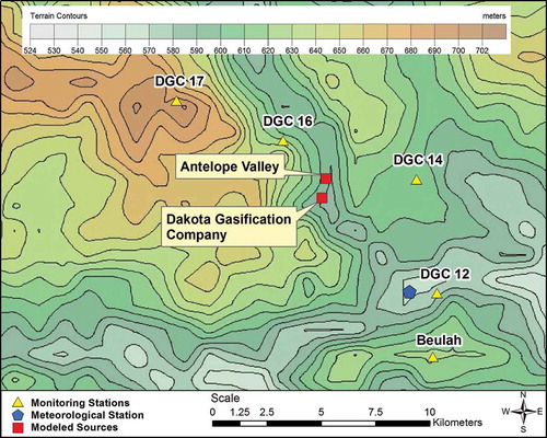
An available 4-year period of 2007–2010 was used for the Mercer County, ND, database with five SO₂ monitors within 10 km of two nearby emission facilities (Antelope Valley and Dakota Gasification Company), site-specific meteorological data at the DGC#12 site (10-m level data in a low-cut grassy field in the location shown in Figure 1), and hourly emissions data from 15 point sources. The terrain in the area is rolling and features three of the monitors (Beulah, DGC#16, and especially DGC#17) being above or close to stack top for some of the nearby emission sources; see Figure 2 for more close-up terrain details. Figure 1 shows a layout of the sources, monitors, and the meteorological station. Tables 2 and 3 provide details about the emission sources and the monitors. Although this modeling application employed sources as far away as 50 km, the proximity of the monitors to the two nearby emission facilities meant that emissions from those facilities dominated the impacts. However, to avoid criticism from reviewers that other regional sources that should have been modeled were omitted, other regional lignite-fired power plants were included in the modeling.

Table 1. Databases selected for the model evaluation.

	Mercer County,	Gibson Generating Station,
	North Dakota	Indiana
Number of emission sources modeled	15	5
Number of SO2 monitors	5	4
	(one above stack top for several sources)	(all below stack top)
Type of terrain	Rolling	Flat
Meteorological years and data source	2007–2010	2008–2010
	Local 10-m tower data	Evansville airport
Meteorological data time step	Hourly and sub-hourly	Hourly and sub-hourly
Emissions and exhaust data	Actual hourly variable emissions and velocity, fixed temperature	Actual hourly variable emissions and velocity, fixed temperature

Table 2. Source information.

Database	Source ID	UTM X (m)	UTM Y (m)	Base elevation (m)	Stack height (m)	Exit temperature (K)	Stack diameter (m)
ND	Antelope Valley	285920	5250189	588.3	182.9	Vary	7.0
ND	Antelope Valley	285924	5250293	588.3	182.9	Vary	7.0
ND	Leland Olds	324461	5239045	518.3	106.7	Vary	5.3
ND	Leland Olds	324557	5238972	518.3	152.4	Vary	6.7
ND	Milton R Young	331870	5214952	597.4	171.9	Vary	6.2
ND	Milton R Young	331833	5214891	600.5	167.6	Vary	9.1
ND	Coyote	286875	5233589	556.9	151.8	Vary	6.4
ND	Stanton	323642	5239607	518.2	77.7	Vary	4.6
ND	Coal Creek	337120	5249480	602.0	201.2	Vary	6.7
ND	Coal Creek	337220	5249490	602.0	201.2	Vary	6.7
ND	Dakota Gasification Company	285552	5249268	588.3	119.8	Vary	7.0
ND	Dakota Gasification Company	285648	5249553	588.3	68.6	Vary	0.5
ND	Dakota Gasification Company	285850	5248600	588.3	76.2	Vary	1.0
ND	Dakota Gasification Company	285653	5249502	588.3	30.5	Vary	0.5
Gibson	Gibson 1	432999	4247189	119.0	189.0	327.2	7.6
Gibson	Gibson 2	432999	4247189	119.0	189.0	327.2	7.6
Gibson	Gibson 3	432923	4247251	118.5	189.0	327.2	7.6
Gibson	Gibson 4	432886	4247340	117.9	152.4	327.2	7.2
Gibson	Gibson 5	432831	4247423	116.3	152.4	327.2	7.2

Notes: SO₂ emission rate and exit velocity vary on hourly basis for each modeled source. Exit temperature varies by hour for the ND sources. UTM zones are 14 for North Dakota and 16 for Gibson.

Figure 1. Map of North Dakota model evaluation layout.

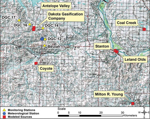
Figure 2. Terrain around the North Dakota monitors.

Gibson Generating Station, Indiana

An available 3-year period of 2008–2010 was used for the Gibson Generating Station in southwest Indiana with four SO₂ monitors within 6 km of the plant, airport hourly meteorological data (from Evansville, IN, 1-min data, located about 40 km SSE of the plant), and hourly emissions data from one electrical generating station (Gibson). The terrain in the area is quite flat and the stacks are tall. Figure 3 depicts the locations of the emission source and the four SO₂ monitors. Although the plant had an on-site meteorological tower, EPA (2013a) noted that the tower’s location next to a large lake resulted in nonrepresentative boundary-layer conditions for the area, and that the use of airport data would be preferred. Tables 2 and 3 provide details about the emission sources and the monitors. Due to the fact that there are no major SO₂ sources within at least 30 km of Gibson, we modeled emissions from only that plant.

Table 3. Monitor locations.

Database	Monitor	UTM X (m)	UTM Y (m)	Monitor elevation (m)
ND	DGC#12	291011	5244991	593.2
ND	DGC#14	290063	5250217	604.0
ND	DGC#16	283924	5252004	629.1
ND	DGC#17^a	279025	5253844	709.8
ND	Beulah	290823	5242062	627.1
Gibson	Mt. Carmel	432424	4250202	119.0
Gibson	East Mt. Carmel	434654	4249666	119.3
Gibson	Shrodt	427175	4247182	138.0
Gibson	Gibson Tower	434792	4246296	119.0

Note: ^aThis monitor’s elevation is above stack top for several of the ND sources.

Figure 3. Map of Gibson model evaluation layout.

Meteorological Data Processing

For the North Dakota and Gibson database evaluations, the hourly surface meteorological data were processed with AERMET, the meteorological preprocessor for AERMOD. The boundary layer parameters were developed according to the guidance provided by EPA in the current AERMOD Implementation Guide (EPA, 2009). For the first modeling evaluation option, Test Case 1, AERMET was run using the default options. For the other four model evaluation options, Test Cases 2 to 5, AERMET was run with the beta u_* low wind speed option.

North Dakota meteorological processing

Four years (2007–2010) of the 10-m meteorological data collected at the DGC#12 monitoring station (located about 7 km SSE of the central emission sources) were processed with AERMET. The data measured at this monitoring station were wind direction, wind speed, and temperature. Hourly cloud cover data from the Dickinson Theodore Roosevelt Regional Airport, North Dakota (KDIK) ASOS station (85 km to the SW), were used in conjunction with the monitoring station data. Upper air data were obtained from the Bismarck Airport, North Dakota (KBIS; about 100 km to the SE), twice-daily soundings.

In addition, the sub-hourly (10-min average) 10-m meteorological data collected at the DGC#12 monitoring station were also processed with AERMET. AERMET was set up to read six 10-min average files with the tower data and output six 10-min average surface and profile files for use in SHARP. SHARP then used the sub-hourly output of AERMET to calculate hourly modeled concentrations, without changing the internal computations of AERMOD. The SHARP user’s manual (EPRI, 2013) provides detailed instructions on processing sub-hourly meteorological data and executing SHARP.

Gibson meteorological processing

Three years (2008–2010) of hourly surface data from the Evansville Airport, Indiana (KEVV), ASOS station (about 40 km SSE of Gibson) were used in conjunction with the twice-daily soundings upper air data from the Lincoln Airport, Illinois (KILX, about 240 km NW of Gibson). The 10-min sub-hourly data for SHARP were generated from the 1-min meteorological data collected at Evansville Airport.

Emission Source Characteristics

Table 2 summarizes the stack parameters and locations of the modeled sources for the North Dakota and Gibson databases. Actual hourly emission rates, stack temperatures, and stack gas exit velocities were used for both databases.

Model Runs and Processing

For each evaluation database, the candidate model configurations were run with hourly emission rates provided by the plant operators. In the case of rapidly varying emissions (startup and shutdown), the hourly averages may average intermittent conditions occurring during the course of the hour. Actual stack heights were used, along with building dimensions used as input to the models tested. Receptors were placed only at the location of each monitor to match the number of observed and predicted concentrations.

The monitor (receptor) locations and elevations are listed in Table 3. For the North Dakota database, the DGC#17 monitor is located in the most elevated terrain of all monitors. The monitors for the Gibson database were located at elevations at or near stack base, with stack heights ranging from 152 to 189 m.

Tolerance Range for Modeling Results

One issue to be aware of regarding SO₂ monitored observations is that they can exhibit over- or underprediction tendencies up to 10% and still be acceptable. This is related to the tolerance in the EPA procedures (EPA, 2013b) associated with quality control checks and span checks of ambient measurements. Therefore, even ignoring uncertainties in model input parameters and other contributions (e.g., model science errors and random variations) that can also lead to modeling uncertainties, just the uncertainty in measurements indicates that modeled-to-monitored ratios between 0.9 and 1.1 can be considered “unbiased.” In the discussion that follows, we consider model performance to be “relatively unbiased” if its predicted model to monitor ratio is between 0.75 and 1.25.

Model Evaluation Metrics

The model evaluation employed metrics that address three basic areas, as described next.

The 1-hr SO₂ NAAQS design concentration

An operational metric that is tied to the form of the 1-hour SO₂ National Ambient Air Quality Standards (NAAQS) is the “design concentration” (99th percentile of the peak daily 1-hr maximum values). This tabulated statistic was developed for each modeled case and for each individual monitor for each database evaluated.

Quantile–quantile plots

Operational performance of models for predicting compliance with air quality regulations, especially those involving a peak or near-peak value at some unspecified time and location, can be assessed with quantile–quantile (Q-Q) plots (Chambers et al., 1983), which are widely used in AERMOD evaluations. Q-Q plots are created by independently ranking (from largest to smallest) the predicted and the observed concentrations from a set of predictions initially paired in time and space. A robust model would have all points on the diagonal (45-degree) line. Such plots are useful for answering the question, “Over a period of time evaluated, does the distribution of the model predictions match those of observations?” Therefore, the Q-Q plot instead of the scatterplot is a pragmatic procedure for demonstrating model performance of applied models, and it is widely used by EPA (e.g., Perry et al. 2005). Venkatram et al. (2001) support the use of Q-Q plots for evaluating regulatory models. Several Q-Q plots are included in this paper in the discussion provided in the following.

Meteorological conditions associated with peak observed versus modeled concentrations

Lists of the meteorological conditions and hours/dates of the top several predictions and observations provide an indication as to whether these conditions are consistent between the model and monitoring data. For example, if the peak observed concentrations generally occur during daytime hours, we would expect that a well-performing model would indicate that the peak predictions are during the daytime as well. Another meteorological variable of interest is the wind speed magnitudes associated with observations and predictions. It would be expected, for example, that if the wind speeds associated with peak observations are low, then the modeled peak predicted hours would have the same characteristics. A brief qualitative summary of this analysis is included in this paper, and supplemental files contain the tables of the top 25 (unpaired) predictions and observations for all monitors and cases tested.

North Dakota Database Model Evaluation Procedures and Results

AERMOD was run for five test cases to compute the 1-hr daily maximum 99th percentile averaged over 4 years at the five ambient monitoring locations listed in Table 3. A regional background of 10 μg/m³ was added to the AERMOD modeled predictions. The 1-hr 99th percentile background concentration was computed from the 2007–2010 lowest hourly monitored concentration among the five monitors so as to avoid double-counting impacts from sources already being modeled.

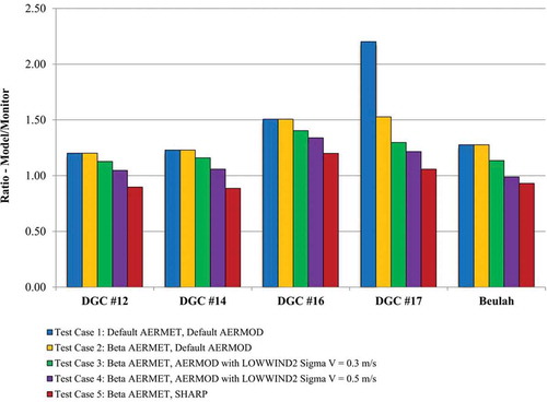
The ratios of the modeled (including the background of 10µg/m³) to monitored design concentrations are summarized in Table 4 and graphically plotted in Figure 4 and are generally greater than 1. (Note that the background concentration is a small fraction of the total concentration, as shown in Table 4.) For the monitors in simple terrain (DGC#12, DGC#14, and Beulah), the evaluation results are similar for both the default and beta options and are within 5–30% of the monitored concentrations depending on the model option. The evaluation result for the monitor in the highest terrain (DGC#17) shows that the ratio of modeled to monitored concentration is more than 2, but when this location is modeled with the AERMET and AERMOD low wind beta options, the ratio is significantly better, at less than 1.3. It is noteworthy that the modeling results for inclusion of just the beta u_* option are virtually identical to the default AERMET run for the simple terrain monitors, but the differences are significant for the higher terrain monitor (DGC#17). For all of the monitors, it is evident that further reductions of AERMOD’s overpredictions occur as the minimum σ_v in AERMOD is increased from 0.3 to 0.5 m/sec. For a minimum σ_v of 0.5 m/sec at all the monitors, AERMOD is shown to be conservative with respect to the design concentration.

Table 4. North Dakota ratio of monitored to modeled design concentrations.

Test case	Monitor	Observed	Predicted	Ratio
Test Case 1 (Default AERMET, Default AERMOD)	DGC#12	91.52	109.96	1.20
	DGC#14	95.00	116.84	1.23
	DGC#16	79.58	119.94	1.51
	DGC#17	83.76	184.48	2.20
	Beulah	93.37	119.23	1.28
Test Case 2	DGC#12	91.52	109.96	1.20
(Beta AERMET, Default AERMOD)	DGC#14	95.00	116.84	1.23
	DGC#16	79.58	119.94	1.51
	DGC#17	83.76	127.93	1.53
	Beulah	93.37	119.23	1.28
Test Case 3	DGC#12	91.52	103.14	1.13
(Beta AERMET, AERMOD with LOWWIND2 σv = 0.3 m/sec)	DGC#14	95.00	110.17	1.16
	DGC#16	79.58	111.74	1.40
	DGC#17	83.76	108.69	1.30
	Beulah	93.37	106.05	1.14
Test Case 4	DGC#12	91.52	95.86	1.05
(Beta AERMET, AERMOD with LOWWIND2 σv = 0.5 m/sec)	DGC#14	95.00	100.50	1.06
	DGC#16	79.58	106.65	1.34
	DGC#17	83.76	101.84	1.22
	Beulah	93.37	92.32	0.99
Test Case 5	DGC#12	91.52	82.18	0.90
(SHARP)	DGC#14	95.00	84.24	0.89
	DGC#16	79.58	95.47	1.20
	DGC#17	83.76	88.60	1.06
	Beulah	93.37	86.98	0.93

Notes: *Design concentration: 99th percentile peak daily 1-hr maximum, averaged over the years modeled and monitored.

Figure 4. North Dakota ratio of monitored to modeled design concentration values at specific monitors.

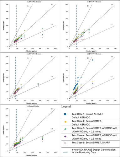
The Q-Q plots of the ranked top fifty daily maximum 1-hr SO₂ concentrations for predictions and observations are shown in Figure 5. For the convenience of the reader, a vertical dashed line is included in each Q-Q plot to indicate the observed design concentration. In general, the Q-Q plots indicate the following:

• For all of the monitors, to the left of the design concentration line, the AERMOD hourly runs all show ranked predictions at or higher than observations. To the right of the design concentration line, the ranked modeled values for specific test cases and monitors are lower than the ranked observed levels, and the slope of the line formed by the plotted points is less than the slope of the 1:1 line. For model performance goals that would need to predict well for the peak concentrations (rather than the 99th percentile statistic), this area of the Q-Q plots would be of greater importance.

• The very highest observed value (if indeed valid) is not matched by any of the models for all of the monitors, but since the focus is on the 99th percentile form of the United States ambient standard for SO₂, this area of model performance is not important for this application.

• The ranked SHARP modeling results are lower than all of the hourly AERMOD runs, but at the design concentration level, they are, on average, relatively unbiased over all of the monitors. The AERMOD runs for SHARP included the meander component, which probably contributed to the small underpredictions noted for SHARP. In future modeling, we would advise users of SHARP to employ the AERMOD LOWWIND1 option to disable the meander component.

Figure 5. North Dakota Q-Q plots: top 50 daily maximum 1-hr SO₂ concentrations: (a) DGC #12 Monitor. (b) DGC#14 monitor. (c) DGC#16 monitor. (d) DGC#17 monitor. (e) Beulah monitor.

Gibson Generating Station Database Model Evaluation Procedures and Results

AERMOD was run for five test cases for this database as well in order to compute the 1-hr daily maximum 99th percentile averaged over three years at the four ambient monitoring locations listed in Table 3. A regional background of 18 μg/m³ was added to the AERMOD modeled predictions. The 1-hr 99th percentile background concentration was computed from the 2008–2010 lowest hourly monitored concentration among the four monitors so as to avoid impacts from sources being modeled.

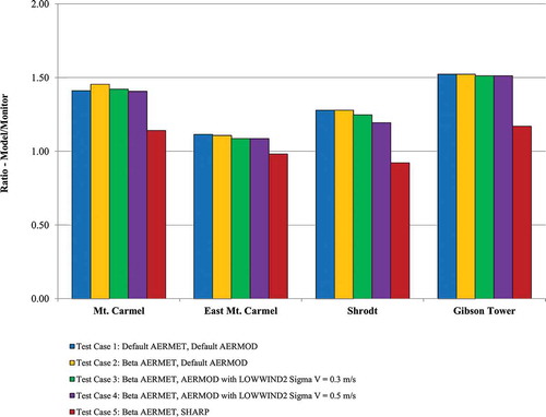
The ratio of the modeled (including the background of 18 µg/m³) to monitored concentrations is summarized in Table 5 and graphically plotted in Figure 6 and are generally greater than 1.0. (Note that the background concentration is a small fraction of the total concentration, as shown in Table 5.) Figure 6 shows that AERMOD with hourly averaged meteorological data overpredicts by about 40–50% at Mt. Carmel and Gibson Tower monitors and by about 9–31% at East Mt. Carmel and Shrodt monitors. As expected (due to dominance of impacts with convective conditions), the AERMOD results do not vary much with the various low wind speed options in this flat terrain setting. AERMOD with sub-hourly meteorological data (SHARP) has the best (least biased predicted-to-observed ratio of design concentrations) performance among the five cases modeled. Over the four monitors, the range of predicted-to-observed ratios for SHARP is a narrow one, ranging from a slight underprediction by 2% to an overprediction by 14%.

Table 5. Gibson ratio of monitored to modeled design concentrations*.

Test case	Monitor	Observed	Predicted	Ratio
Test Case 1	Mt. Carmel	197.25	278.45	1.41
(Default AERMET, Default AERMOD)	East Mt. Carmel	206.89	230.74	1.12
	Shrodt	148.16	189.63	1.28
	Gibson Tower	127.12	193.71	1.52
Test Case 2	Mt. Carmel	197.25	287.16	1.46
(Beta AERMET, Default AERMOD)	East Mt. Carmel	206.89	229.22	1.11
	Shrodt	148.16	189.63	1.28
	Gibson Tower	127.12	193.71	1.52
Test Case 3	Mt. Carmel	197.25	280.32	1.42
(Beta AERMET, AERMOD with LOWWIND2 σv = 0.3 m/sec)	East Mt. Carmel	206.89	224.65	1.09
	Shrodt	148.16	184.82	1.25
	Gibson Tower	127.12	192.22	1.51
Test Case 4	Mt. Carmel	197.25	277.57	1.41
(Beta AERMET, AERMOD with LOWWIND2 σv = 0.5 m/sec)	East Mt. Carmel	206.89	224.65	1.09
	Shrodt	148.16	176.81	1.19
	Gibson Tower	127.12	192.22	1.51
Test Case 5	Mt. Carmel	197.25	225.05	1.14
(SHARP)	East Mt. Carmel	206.89	202.82	0.98
	Shrodt	148.16	136.41	0.92
	Gibson Tower	127.12	148.64	1.17

Notes: *Design Concentration: 99^th percentile peak daily 1-hr maximum, averaged over the years modeled and monitored.

Figure 6. Gibson ratio of monitored to modeled design concentration values at specific monitors.

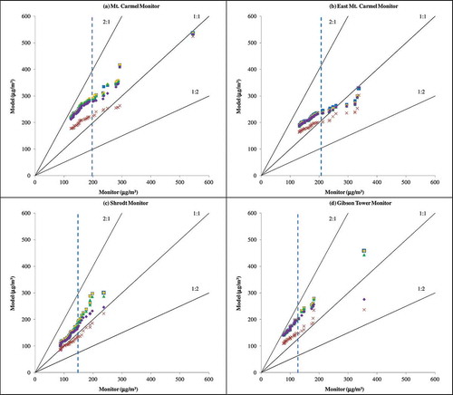
The Q-Q plots of the ranked top fifty daily maximum 1-hr SO₂ concentrations for predictions and observations are shown in Figure 7. It is clear from these plots that the SHARP results parallel and are closer to the 1:1 line for a larger portion of the concentration range than any other model tested. In general, AERMOD modeling with hourly data exhibits an overprediction tendency at all of the monitors for the peak ranked concentrations at most of the monitors. The AERMOD/SHARP models predicted lower relative to observations at the East Mt. Carmel monitor for the very highest values, but match well for the 99th percentile peak daily 1-hr maximum statistic.

Figure 7. Gibson Q-Q plots: top 50 daily maximum 1-hour SO₂ concentrations. (a) Mt. Carmel monitor. (b) East Mt. Carmel monitor. (c) Shrodt monitor. (d) Gibson tower monitor. For the legend, see Figure 5.

Evaluation Results Discussion

The modeling results for these tall stack releases are sensitive to the source local setting and proximity to complex terrain. In general, for tall stacks in simple terrain, the peak ground-level impacts mostly occur in daytime convective conditions. For settings with a mixture of simple and complex terrain, the peak impacts for the higher terrain are observed to occur during both daytime and nighttime conditions, while AERMOD tends to favor stable conditions only without low wind speed enhancements. Exceptions to this “rule of thumb” can occur for stacks with aerodynamic building downwash effects. In that case, high observed and modeled predictions are likely to occur during high wind events during all times of day.

The significance of the changes in model performance for tall stacks (using a 90th percentile confidence interval) was independently tested for a similar model evaluation conducted for Eastman Chemical Company (Paine et al., 2013; Szembek et al., 2013), using a modification of the Model Evaluation Methodology (MEM) software that computed estimates of the hourly stability class (Strimaitis et al., 1993). That study indicated that relative to a perfect model, a model that overpredicted or underpredicted by less than about 50% would likely show a performance level that was not significantly different. For a larger difference in bias, one could expect a statistically significant difference in model performance. This finding has been adopted as an indicator of the significance of different modeling results for this study.

A review of the North Dakota ratios of monitored to modeled values in Figure 4 generally indicates that for DGC#12, DGC#14, and Beulah, the model differences were not significantly different. For DGC#16, it could be concluded that the SHARP results were significantly better than the default AERMOD results, but other AERMOD variations were not significantly better. For the high terrain monitor, DGC#17, it is evident that all of the model options departing from default were significantly better than the default option, especially the SHARP approach.

For the Gibson monitors (see Figure 6), the model variations did not result in significantly different performance except for the Gibson Tower (SHARP vs. the hourly modes of running AERMOD).

General conclusions from the review of meteorological conditions associated with the top observed concentrations at the North Dakota monitors, provided in the supplemental file called “North Dakota Meteorological Conditions Resulting in Top 25 Concentrations,” are as follows:

• A few peak observed concentrations occur at night with light winds. The majority of observations for the DGC#12 monitor are mostly daytime conditions with moderate to strong winds.

• Peak observations for the DGC#14 and Beulah monitors are mostly daytime conditions with a large range of wind speeds. Once again, a minority of the peak concentrations occur at night with a large range of wind speeds.

• Peak observed concentrations for the DGC#16 and DGC#17 monitors occur at night with light winds. Majority of observations are mixed between daytime and nighttime conditions with a large range of wind speeds for both. The DGC#17 monitor is located in elevated terrain.

The conclusions from the review of the meteorological conditions associated with peak AERMOD or SHARP predictions are as follows:

• AERMOD hourly peak predictions for the DGC#12 and Beulah monitors are consistently during the daytime with light to moderate wind speeds and limited mixing heights. This is a commonly observed situation that is further discussed later.

• There are similar AERMOD results for DGC#14, except that there are more periods with high winds and higher mixing heights.

• The AERMOD results for DGC#16 still feature mostly daytime hours, but with more high wind conditions.

• The default AERMOD results for DGC#17 are distinctly different from the other monitors, with most hours featuring stable, light winds. There are also a few daytime hours of high predictions with low winds and low mixing heights. This pattern changes substantially with the beta u_* options employed, when the majority of the peak prediction hours are daytime periods with light to moderate wind speeds. This pattern is more consistent with the peak observed concentration conditions.

• The SHARP peak predictions at the North Dakota monitors were also mostly associated with daytime hours with a large range of wind speeds for all of the monitors.

The North Dakota site has some similarities due to a mixture of flat and elevated terrain to the Eastman Chemical Company model evaluation study in Kingsport, TN (this site features three coal-fired boiler houses with tall stacks). In that study (Paine et al. 2013; Szembek et al., 2013), there was one monitor in elevated terrain and two monitors in flat terrain with a full year of data. Both the North Dakota and Eastman sites featured observations of the design concentration being within about 10% of the mean design concentration over all monitors. Modeling results using default options in AERMOD for both of these sites indicated a large spread of the predictions, with predictions in high terrain exceeding observations by more than a factor of 2. In contrast, the predictions in flat terrain, while higher than observations, showed a lower overprediction bias. The use of low wind speed improvements in AERMOD (beta u_* in AERMET and an elevated minimum σ_v value) did improve model predictions for both databases.

The conclusions from the review of the meteorological conditions associated with peak observations, provided in the supplemental file called “Gibson Meteorological Conditions Resulting in Top 25 Concentrations,” are as follows:

• Peak observations for the Mt. Carmel and East Mt. Carmel monitors occur during both light wind convective conditions and strong wind conditions (near neutral, both daytime and nighttime).

• Nighttime peaks that are noted at Mt. Carmel and East Mt. Carmel could be due to downwash effects with southerly winds.

• Gibson Tower and Shrodt monitors were in directions with minimal downwash effects; therefore, the peak impacts at these monitors occur with convective conditions.

• The Gibson Tower and Shrodt monitor peak observation conditions were similarly mixed for wind speeds, but they were consistently occurring during the daytime only.

AERMOD (hourly) modeling runs and SHARP runs are generally consistent with the patterns of observed conditions for Shrodt and Gibson Tower monitors. Except for downwash effects, the peak concentrations were all observed and predicted during daytime hours. There are similar AERMOD results for Mt. Carmel and East Mt. Carmel, except that there are more nighttime periods and periods with strong wind conditions.

As noted earlier, AERMOD tends to focus its peak predictions for tall stacks in simple terrain (those not affected by building downwash) for conditions with low mixing heights in the morning. However, a more detailed review of these conditions indicates that the high predictions are not simply due to plumes trapped within the convective mixed layer, but instead due to plumes that initially penetrate the mixing layer, but then emerge (after a short travel time) into the convective boundary layer in concentrated form with a larger-than-expected vertical spread. Tests of this condition were undertaken by Dr. Ken Rayner of the Western Australia Department of Environmental Regulation (2013), who found the same condition occurring for tall stacks in simple terrain for a field study database in his province. Rayner found that AERMOD tended to overpredict peak concentrations by a factor of about 50% at a key monitor, while with the penetrated plume removed from consideration, AERMOD would underpredict by about 30%. Therefore, the correct treatment might be a more delayed entrainment of the penetrated plume into the convective mixed layer. Rayner’s basic conclusions were:

• A plume penetrates and disperses within a 1-hr time step in AERMOD, while in the real world, dispersion of a penetrated puff may occur an hour or more later, after substantial travel time.

• A penetrated plume initially disperses via a vertical Gaussian formula, not a convective probability density function. Because penetrated puffs typically have a very small vertical dispersion, they are typically fully entrained (in AERMOD) in a single hour by a growing mixed layer, and dispersion of a fully entrained puff is via convective mixing, with relatively rapid vertical dispersion, and high ground-level concentrations.

Conclusions and Recommendations for Further Research

This study has addressed additional evaluations for low wind conditions involving tall stack releases for which multiple years of concurrent emissions, meteorological data, and monitoring data were available. The modeling cases that were the focus of this study involved applications with only one level of meteorological data and no direct turbulence measurements or vertical temperature gradient observations.

For the North Dakota evaluation, the AERMOD model overpredicted, using the design concentration as the metric for each monitor. For the relatively low elevation monitors, the results were similar for both the default and beta options and are within 5–30% of the monitored concentrations depending on the model option. The modeling result for the elevated DGC#17 monitor showed that this location is sensitive to terrain, as the ratio of modeled to monitored concentration is over 2. However, when this location was modeled with the low wind beta option, the ratio was notably better, at less than 1.3. Furthermore, the low wind speed beta option changed the AERMOD’s focus on peak predictions conditions from mostly nighttime to mostly daytime periods, somewhat more in line with observations. Even for a minimum σ_v as high as 0.5 m/sec, all of the AERMOD modeling results were conservative or relatively unbiased (for the design concentration). The North Dakota evaluation results for the sub-hourly (SHARP) modeling were, on average, relatively unbiased, with a predicted-to-observed design concentration ratio ranging from 0.89 to 1.2. With a 10% tolerance in the SO₂ monitored values, we find that the SHARP performance is quite good. Slightly higher SHARP predictions would be expected if AERMOD were run with the LOWWIND1 option deployed.

For the Gibson flat terrain evaluation, AERMOD with hourly averaged meteorological data overpredicted at three of the four monitors between 30 and 50%, and about 10% at the fourth monitor. The AERMOD results did not vary much with the various low wind speed options in this flat terrain setting. AERMOD with sub-hourly meteorological data (SHARP) had the best (least biased predicted-to-observed ratio of design concentrations) performance among the five cases modeled. Over the four monitors, the range of predicted-to-observed ratios for SHARP was a narrow one, ranging from a slight underprediction by 2% to an overprediction by 14%. All other modeling options had a larger range of results.

The overall findings with the low wind speed testing on these tall stack databases indicate that:

• The AERMOD low wind speed options have a minor effect for flat terrain locations.

• The AERMOD low wind speed options have a more significant effect with AERMOD modeling for elevated terrain locations, and the use of the LOWWIND2 option with a minimum σ_v on the order of 0.5 m/sec is appropriate.

• The AERMOD sub-hourly modeling (SHARP) results are mostly in the unbiased range (modeled to observed design concentration ratios between 0.9 and 1.1) for the two databases tested with that option.

• The AERMOD low wind speed options improve the consistency of meteorological conditions associated with the highest observed and predicted concentration events.

Further analysis of the low wind speed performance of AERMOD with either the SHARP procedure or the use of the minimum σ_v specifications by other investigators is encouraged. However, SHARP can only be used if sub-hourly meteorological data is available. For Automated Surface Observing Stations (ASOS) with 1-min data, this option is a possibility if the 1-min data are obtained and processed.

Although the SHARP results reported in this paper are encouraging, further testing is recommended to determine the optimal sub-hourly averaging time (no less than 10 min is recommended) and whether other adjustments to AERMOD (e.g., total disabling of the meander option) are recommended. Another way to implement the sub-hourly information in AERMOD and to avoid the laborious method of running AERMOD several times for SHARP would be to include a distribution, or range, of the sub-hourly wind directions to AERMOD so that the meander calculations could be refined.

For most modeling applications that use hourly averages of meteorological data with no knowledge of the sub-hourly wind distribution, it appears that the best options with the current AERMOD modeling system are to implement the AERMET beta u_* improvements and to use a minimum σ_v value on the order of 0.5 m/sec/sec.

It is noteworthy that EPA has recently approved (EPA, 2015) as a site-specific model for Eastman Chemical Company the use of the AERMET beta u_* option as well as the LOWWIND2 option in AERMOD with a minimum σ_v of 0.4 m/sec. This model, which was evaluated with site-specific meteorological data and four SO₂ monitors operated for 1 year, performed well in flat terrain, but overpredicted in elevated terrain, where a minimum σ_v value of 0.6 m/sec actually performed better. This would result in an average value of the minimum σ_v of about 0.5 m/sec, consistent with the findings of Hanna (1990).

The concept of a minimum horizontal wind fluctuation speed on the order of about 0.5 m/sec is further supported by the existence of vertical changes (shears) in wind direction (as noted by Etling, 1990) that can result in effective horizontal shearing of a plume that is not accounted for in AERMOD. Although we did not test this concept here, the concept of vertical wind shear effects, which are more prevalent in decoupled stable conditions than in well-mixed convective conditions, suggests that it would be helpful to have a “split minimum σ_v” approach in AERMOD that enables the user to specify separate minimum σ_v values for stable and unstable conditions. This capability would, of course, be backward-compatible to the current minimum σ_v specification that applies for all stability conditions in AERMOD now.

Supplemental Material

Supplemental data for this article can be accessed at the publisher’s website

Additional information

Notes on contributors

Robert Paine

Robert Paine, CCM, QEP, is an associate vice-president and technical director and Olga Samani and Mary Kaplan are senior air quality meteorologists with AECOM’s Air Quality Modeling group in Chelmsford, MA.

Eladio Knipping

Eladio Knipping is a principal technical leader in the Environment Sector at the Electric Power Research Institute office in Washington, DC.

Naresh Kumar

Naresh Kumar is a senior program manager of air quality in the environment sector at the Electric Power Research Institute office in Palo Alto, CA.

References

- Anfossi, D., D. Oettl, G. Degrazia, and A. Goulart. 2005. An analysis of sonic anemometer observations in low wind speed conditions. Boundary Layer Meteorol. 114:179–203. doi:10.1007/s10546-004-1984-4
- Barad, M.L. 1958. Project Prairie Grass, a field program in diffusion. Geophys. Res. Pap. 59. Bedford, MA: Air Force Cambridge Centre.
- Brett, A.C., and S.E. Tuller. 1991. The autocorrelation of hourly wind speed observations. J. Appl. Meteorol. 30:823–33. doi:10.1175/1520-0450(1991)030%3C0823:TAOHWS%3E2.0.CO;2
- Chambers, J.M., W.S. Cleveland, B. Kleiner, and P.A. Tukey. 1983. Comparing data distributions. Graphical methods for data analysis. Pacific Grove, CA: Bell Laboratories. Wadsworth International Group and Duxbury Press.
- Chowdhury, B., R.I. Sykes, D. Henn, and P. Karamchandani. 2014. SCICHEM Version 3.0 (Beta 2) technical documentation. http://sourceforge.net/projects/epri-dispersion/files/SCICHEM/SCICHEM3.0b2.zip/download
- Cimorelli, A.J., S.G. Perry, A. Venkatram, J.C. Weil, R.J. Paine, R.B. Wilson, R.F. Lee, W.D. Peters, and R.W. Brode. 2005. AERMOD: A dispersion model for industrial source applications. Part I: General model formulation and boundary layer characterization. J. Appl. Meteorol. 44:682–93. doi:10.1175/JAM2227.1
- Electric Power Research Institute. 2013. Sub Hourly AERMOD Run Procedure (SHARP), version 13011 user’s guide. Research project 1025622. http://sourceforge.net/projects/epri-dispersion/files/SHARP (accessed June 10, 2015).
- Etling, D. 1990. On plume meandering under stable stratification. Atmos. Environ. 8:1979–85. doi:10.1016/0960-1686(90)90232-C
- Hanna, S.R. 1990. Lateral dispersion in light-wind stable conditions, Nuovo Cimento 13:889–94. doi:10.1007/BF02514777
- Irwin, J.S. 2014. A suggested method for dispersion model evaluation. J. Air Waste Manage. Assoc. 64(3):255–64. doi:10.1080/10962247.2013.833147
- Kaplan, M., and R.J. Paine. 2012. Comparison of AERMOD modeled 1-hour SO2 concentrations to observations at multiple monitoring stations in North Dakota. Presented at the 105th Annual Conference and Exhibition of the Air & Waste Management Association, June 2012, San Antonio, TX.
- Luhar, A.K., and K.N. Rayner. 2009. Methods to estimate surface fluxes of momentum and heat from routine weather observations for dispersion applications under stable stratification. Boundary Layer Meteorol. 132:437–54. doi:10.1007/s10546-009-9409-z
- Mahrt, L. 1998. Stratified atmospheric boundary layers and breakdown of models. Theor. Comput. Fluid Dynam. 11:263–79. doi:10.1007/s001620050093
- Paine, R., J.A. Connors, and C.D. Szembek, 2010. AERMOD low wind speed evaluation study: Results and implementation. Paper 2010-A-631-AWMA. Presented at the 103rd Annual Conference, Air & Waste Management Association, June 2012, Calgary, Alberta, Canada.
- Paine, R., F. Tringale, and S. Gossett, 2013. Resolution of 1-hour SO2 non-attainment area in Kingsport, TN: Advanced meteorological and monitoring study. Presented at the Air & Waste Management Association’s Specialty Conference. Raleigh, NC, March.
- Pasquill, F., and F.B. Smith. 1983. Atmospheric Diffusion. Series in Environmental Science. Ellis Horwood. Chichester: John Wiley & Sons.
- Perez, I., M. Garcia, M. Sanchez, and B. De Torre. 2004. Autocorrelation analysis of meteorological data from a RASS Sodar. J. Appl. Meteorol., 43:1213–23. doi:10.1175/1520-0450(2004)043%3C1213:AAOMDF%3E2.0.CO;2
- Perry, S.G., A.J. Cimorelli, R.J. Paine, R.W. Brode, J.C. Weil, A. Venkatram, R.B. Wilson, R.F. Lee, and W.D. Peters. 2005. AERMOD: A dispersion model for industrial source applications. Part II: Model performance against 17 field study databases. J. Appl. Meteorol. 44:694–708. doi:10.1175/JAM2228.1
- Qian, W., and A. Venkatram. 2011. Performance of steady-state dispersion models under low wind-speed conditions. Boundary Layer Meteorol. 138:475–91. doi:10.1007/s10546-010-9565-1
- Rayner, K. 2013. Personal communication with Robert Paine, AECOM.
- Sagendorf, J.F., and C.R. Dickson. 1974. Diffusion under low windspeed, inversion conditions. NOAA Technical Memorandum 52. http://www.arl.noaa.gov/documents/reports/ARL-52.pdf (accessed September 9, 2015).
- Smedman, A.S. 1988. Observations of a multi-level turbulence structure in a very stable atmospheric boundary layer. Boundary Layer Meteorol. 66:105–26. doi:10.1007/BF00116064
- Strimaitis, D., E. Insley, M. Korc, and F. Lurmann. 1993. User’s guide for the Model Evaluation Methodology (MEM) system for comparing model performance, Version 1.0. STI-93261-1392-FR. Prepared for U.S. Environmental Protection Agency, Research Triangle Park, NC.
- Szembek, C., R. Paine, and S. Gossett. 2013. Resolution of 1-hour SO2 non-attainment area in Kingsport, TN: Model evaluation analysis results to date. Presented at the Air & Waste Management Association’s Specialty Conference, Raleigh, NC, March.
- U.S. Environmental Protection Agency. 2004. AERMOD: Description of model formulation. EPA-454/R-03-004. http://www.epa.gov/ttn/scram/7thconf/aermod/aermod_mfd.pdf (accessed June 10, 2015).
- U.S. Environmental Protection Agency. 2005. Revision to the guideline on air quality models: Adoption of a preferred general purpose (flat and complex terrain) dispersion model and other revisions. Final rule. Fed. Reg. 70 (216). http://www.gpo.gov/fdsys/pkg/FR-2005-11-09/html/05-21627.htm (accessed June 10, 2015).
- U.S. Environmental Protection Agency. 2009. AERMOD implementation guide (AIG). http://www.epa.gov/ttn/scram/7thconf/aermod/aermod_implmtn_guide_19March2009.pdf (accessed June 10, 2015).
- U.S. Environmental Protection Agency. 2012. AERMET 12345 model change bulletin MCB#3. http://www.epa.gov/ttn/scram/7thconf/aermod/aermet_mcb3.txt (accessed June 10, 2015).
- U.S. Environmental Protection Agency. 2013a. Personal communication from Roger Brode, EPA, to Robert Paine, AECOM.
- U.S. Environmental Protection Agency. 2013b. Quality Assurance Handbook for Air Pollution Measurement Systems, Volume II, Ambient Air Quality Monitoring Program. http://www.epa.gov/ttnamti1/files/ambient/pm25/qa/QA-Handbook-Vol-II.pdf (accessed June 10, 2015).
- U.S. Environmental Protection Agency. 2014a. Webinar: AERMOD modeling system update, January 15. http://www.epa.gov/ttn/scram/webinar/AERMOD_13350_Update/AERMOD_System_Update_Webinar_01-14-2014_FINAL.pdf (accessed June 10, 2015).
- U.S. Environmental Protection Agency. 2014b. Webinar: AERMOD modeling system update, August 14. http://www.epa.gov/ttn/scram/webinar/AERMOD_14134-NO2_Memo/20140812-Webinar_Slides.pdf (accessed June 10, 2015).
- U.S. Environmental Protection Agency. 2015. Approval of alternative model request: Modeling of sulfur dioxide emissions from Eastman Chemical Company, Sullivan County, Tennessee, 2010 Sulfur dioxide National Ambient Air Quality Standards (NAAQS) nonattainment area. Letter to Mr. Barry R. Stephens, Tennessee Department of Environment and Conservation from Beverly H. Bannister, Director of Air, Pesticides and Toxics Management Division (EPA Region 4).
- Van der Hoven, I. 1976. A survey of field measurements of atmospheric diffusion under low-wind-speed inversion conditions. Nuclear Safety 17:223–30.
- Venkatram, A., R.W. Brode, A.J. Cimorelli, J.T. Lee, R.J. Paine, S.G. Perry, W.D. Peters, J.C. Weil, and R.B. Wilson. 2001. A complex terrain dispersion model for regulatory applications. Atmos. Environ. 35:4211–21. doi:10.1016/S1352-2310(01)00186-8
- Wilson, R.B., G.E. Start, C.R. Dickson, and N.R. Ricks. 1976. Diffusion under low wind speed conditions near Oak Ridge, Tennessee. NOAA Technical Memorandum ERL ARL-61, 83 pp. http://www.arl.noaa.gov/documents/reports/ARL-61.pdf (accessed September 9, 2015).