Applications of GPS-tracked personal and fixed-location PM_2.5 continuous exposure monitoring

ABSTRACT

Continued development of personal air pollution monitors is rapidly improving government and research capabilities for data collection. In this study, we tested the feasibility of using GPS-enabled personal exposure monitors to collect personal exposure readings and short-term daily PM_2.5 measures at 15 fixed locations throughout a community. The goals were to determine the accuracy of fixed-location monitoring for approximating individual exposures compared to a centralized outdoor air pollution monitor, and to test the utility of two different personal monitors, the RTI MicroPEM V3.2 and TSI SidePak AM510. For personal samples, 24-hr mean PM_2.5 concentrations were 6.93 μg/m³ (stderr = 0.15) and 8.47 μg/m³ (stderr = 0.10) for the MicroPEM and SidePak, respectively. Based on time–activity patterns from participant journals, exposures were highest while participants were outdoors (MicroPEM = 7.61 µg/m³, stderr = 1.08, SidePak = 11.85 µg/m³, stderr = 0.83) or in restaurants (MicroPEM = 7.48 µg/m³, stderr = 0.39, SidePak = 24.93 µg/m³, stderr = 0.82), and lowest when participants were exercising indoors (MicroPEM = 4.78 µg/m³, stderr = 0.23, SidePak = 5.63 µg/m³, stderr = 0.08). Mean PM_2.5 at the 15 fixed locations, as measured by the SidePak, ranged from 4.71 µg/m³ (stderr = 0.23) to 12.38 µg/m³ (stderr = 0.45). By comparison, mean 24-h PM_2.5 measured at the centralized outdoor monitor ranged from 2.7 to 6.7 µg/m³ during the study period. The range of average PM_2.5 exposure levels estimated for each participant using the interpolated fixed-location data was 2.83 to 19.26 µg/m³ (mean = 8.3, stderr = 1.4). These estimated levels were compared with average exposure from personal samples. The fixed-location monitoring strategy was useful in identifying high air pollution microclimates throughout the county. For 7 of 10 subjects, the fixed-location monitoring strategy more closely approximated individuals’ 24-hr breathing zone exposures than did the centralized outdoor monitor. Highlights are: Individual PM_2.5 exposure levels vary extensively by activity, location and time of day; fixed-location sampling more closely approximated individual exposures than a centralized outdoor monitor; and small, personal exposure monitors provide added utility for individuals, researchers, and public health professionals seeking to more accurately identify air pollution microclimates.

Implications: Personal air pollution monitoring technology is advancing rapidly. Currently, personal monitors are primarily used in research settings, but could they also support government networks of centralized outdoor monitors? In this study, we found differences in performance and practicality for two personal monitors in different monitoring scenarios. We also found that personal monitors used to collect outdoor area samples were effective at finding pollution microclimates, and more closely approximated actual individual exposure than a central monitor. Though more research is needed, there is strong potential that personal exposure monitors can improve existing monitoring networks.

Introduction

Fine airborne particulate matter of less than 2.5 μm (PM_2.5) is formed primarily by combustion of fuels, is thought to be involved in causal disease pathways for asthma, cardiovascular disease, and lung cancer, and can also increase susceptibility to infectious diseases (Gamble, 1998; Adams et al., 2001; Sorensen et al., 2003; Brook et al., 2010; Glad et al., 2012; Sloan et al., 2012; Stern et al., 2013; Das et al., 2014; Lippmann, 2014). PM_2.5 is not easily cleared by inertial impaction in the nasopharynx or by ciliary action in the trachea, bronchi, and bronchioles, and thus can travel to the lower airways, causing inflammation leading to respiratory epithelial damage (Anderson et al., 2012; Eide and Lillquist, 2003; Fann et al., 2012). Due to the variety of adverse health effects caused by PM_2.5 and other air contaminants, air pollution is estimated to be responsible for as many as 130,000 deaths per year in the United States (800,000 worldwide) with nearly 1.1 million life years lost (Anderson et al., 2012; Fann et al., 2012).

The Environmental Protection Agency (EPA) and many private agencies conduct measurements of outdoor air pollution at monitoring stations across the country (Miranda et al., 2011). While outdoor monitors provide useful information regarding ambient pollution levels, they do not accurately estimate individuals’ daily exposures. Particulate levels vary a great deal in local areas (microclimates), depending on the density of transmission sources, weather, and altitude (Gulliver and Briggs, 2004; Zuurbier et al., 2010; Zuurbier et al., 2011; Breen et al., 2014). Even for individuals who live at the same residence, exposure can differ by more than 30% in a single day (Dons, Int Panis et al., 2011). Further, most people spend between 69 and 90% of their day indoors, while stationary monitors are only able to capture data at a single outdoor location (Klepeis et al., 2001; Dales et al., 2008; Zuurbier et al., 2010; Dons et al., 2011; Hochstetler et al., 2011; Steinle et al., 2011; Hasenfratz et al., 2012; Steinle et al., 2013). Even stationary monitors placed directly in homes do not correlate well with actual particulate exposure in the home when compared to measurements taken in an individual’s breathing zone (Steinle et al., 2013).

Ideally, exposure to atmospheric pollutants should be estimated from personal breathing zone samples to account for variation in individuals’ time–activity–location patterns; however, this sampling strategy is not currently feasible for large numbers of people living within a community. Conversely, population-level exposure estimates made from centralized outdoor air pollution monitors are poorly correlated with personal exposures (Avery et al., 2010; Wheeler et al., 2011). Furthermore, exposure-modeling approaches have been limited by a lack of accurate data on individual time–activity–location patterns and inaccuracies associated with estimating microclimate pollution levels (Dias and Tchepel, 2014; Breen et al., 2014). Recent advances in global positioning system (GPS) and geographical information system (GIS) technologies, however, now allow for highly resolved measurement of individuals’ time–location patterns, which may significantly improve air pollution exposure estimates. For instance, GPS-equipped mobile phones have been used to enhance exposure models by improving spatiotemporal measurement of participants’ movements though air pollution microclimates (Dias and Tchepel, 2014; Gu et al., 2015).

Similarly, many companies are now developing small personal air pollution exposure monitors to obtain more accurate readings of daily exposures; many of these monitors are in the prototype stage (Steinle et al., 2013). Personal monitoring has the advantage of being able to track individuals’ air pollution exposures as they travel through outdoor and indoor microclimates; however, this sampling method has been limited in the past due to the size, weight, and noise produced by the equipment. Combined approaches are also becoming more common, where researchers and companies are pairing personal exposure monitors with GPS units so real-time exposure information can be pinpointed to individual locations (Dons et al., 2011; Berrio et al., 2013). GPS loggers have also been used alone or in combination with personal air pollution monitors to validate exposure models (Dons et al., 2014) (Gerharz et al., 2013; Breen et al., 2014). While multiple studies have shown personal monitoring to more accurately represent air pollution exposures than centralized outdoor monitors (e.g., Rodes et al., 2010; Wheeler et al., 2011), more research is needed to determine how these new instruments can be most effectively used to supplement or improve current ambient air pollution monitoring programs.

In this study, we tested the utility of GPS-enabled personal exposure monitors to measure outdoor microclimate variation at multiple fixed locations within a community, and to determine whether this monitoring strategy more closely approximates individuals’ breathing zone PM_2.5 exposures compared to a centralized outdoor air pollution monitor. To test this sampling strategy, we compared two personal exposure monitors, the MicroPEM (RTI International, Research Triangle Park, NC; Rodes et al., 2012) and the SidePak AM510 (TSI, Inc., Shoreview, MN) for measuring both personal breathing zone and outdoor fixed-location PM_2.5 levels. Measurements were taken in Utah County, Utah, which is located along the Wasatch Mountain Range. This area is known to experience high PM_2.5 levels due to high traffic volume and its valley location, which prevents wind dispersal (Pope, 1991; Pope et al., 1992; Pope, 1995; Brook et al., 2010).

Materials and methods

In this study, GPS tracking and breathing zone PM_2.5 concentrations were measured for 10 participants recruited from among faculty and staff at Brigham Young University. All participants lived in Utah County, Utah, and were nonsmokers. Exposure monitoring was performed during September 4–October 22, 2014. Participants consented to wear the exposure monitors and GPS unit for a continuous 24-hr period on weekdays while conducting their normal activities. The vest was removed but kept near the participants while sleeping, showering, or performing other activities that did not allow for the vest to be worn. Participants maintained a time–activity diary where they recorded their activities in 15-min intervals during the sampling period. They were instructed to describe their activity on the journal each 15 minutes rather than waiting, so recall bias was negligible. In addition, study personnel measured PM_2.5 concentrations twice per week at purposefully selected locations throughout the county. All study procedures and materials were approved by the Institutional Review Board at Brigham Young University. The sampling is described in more detail in the following.

Personal monitoring

PM_2.5 exposures were measured continuously over a 24-hr sampling period for each participant (n = 10) using an RTI MicroPEM V3.2 and TSI SidePak AM510 personal exposure monitor. All individuals resided within Utah County, with representatives from most of its major municipalities. The MicroPEM allows for integrated (gravimetric) sampling while simultaneously collecting real-time, data-logged PM_2.5 measurements using an on-board 780-nm infrared (IR) laser nephelometer operating on a 10.0-sec cycling time. MicroPEMs are limited to a 36- to 40-hr continuous operating time on AA alkaline batteries at a 0.50-L/min flow rate. Due to the short duration of this study, a battery change-out schedule was not required. Prior to data collection, MicroPEMs were fitted with a two-stage mini-impactor set with initial and final cutpoints at 4.0 μm and 2.5 μm, respectively. Sintered stainless-steel impaction plates were lubricated with silicone oil. Preweighed 3.0-µm polytetrafluoroethylene (PTFE) 25-mm TEFLO filters (Zefon International, Ocala, FL) were placed in MicroPEM filter cassettes during sampling. MicroPEMs were zeroed with an in-line HEPA filter, and precalibrated at 0.50 L/min with a TSI model 4140 mass flowmeter (TSI, Inc., Shoreview, MN) using Docking Station software (RTI International, Research Triangle Park, NC). Although the MicroPEM allows for gravimetric and chemical analysis of air pollution constituents, the low flow rate, short sampling duration, and relatively low PM_2.5 concentrations encountered in this study resulted in little particulate mass on the filters. Thus, we were limited to using nephelometer readings to estimate personal and fixed-location PM_2.5 concentrations.

The TSI SidePak data-logged PM_2.5 concentration every 10.0 sec using a 670-nm laser calibrated to ISO 12103-1 A1 test dust (Arizona dust). Prior to data collection, SidePaks were fitted with an internal PM_2.5 impactor, zeroed with an in-line HEPA filter, and calibrated to 1.70 L/min flow rate using a Defender 510 volumetric primary flow standard (Mesa Labs, Butler, NJ). Impaction plates were cleaned and coated with vacuum grease after each 24-hr sampling period. To extend the run time of the SidePAK instruments we used the 6-cell AA alkaline battery pack option, which provided approximately 22.5 hr of continuous sampling at the 1.7 L/min flow rate. SidePAKs ran continuously until the batteries died with no change-out schedule. The SidePAK AM510 does not allow for integrated, filter-based sampling. We were thus limited to time-series PM_2.5 concentrations, and were unable to characterize air pollution constituents. The SidePAKs produced considerably more noise than the MicroPEMs, which may limit their use in future air pollution studies.

A sampling vest was designed for use in this study to ensure placement of the MicroPEM and SidePak inlets in the participants’ breathing zone. Breathing zone was defined as the sphere of air located within a 25-cm (10-in) radius of the participant’s nostrils (DiNardi and American Industrial Hygiene Association [AIHA], 2003). The MicroPEM was held in an upright, vertical position near the participant’s collarbone in a breathable mesh pocket sewn into the vest, and secured by an elastic strap. The inlet housing extended outside of the pocket, where it was exposed to ambient air. Participants were instructed to wear the sampling vest throughout the 24-hr period with the exception of sleep time, for which they were instructed to place the vest near their bed. The SidePak was also held in the vest in an upright position, with Tygon tubing extending from the SidePak to the participants’ breathing zone. Sampling vests were made from ripstop nylon with nylon belting. Nylon fabric was chosen because it releases low levels of particles compared to other fabrics, thereby reducing bias when collecting breathing zone measurements (Williams et al., 2003). A photo of the measurement vest is included as Figure S1.

Fixed-location sampling

Study personnel performed PM_2.5 sampling twice per week at predetermined locations in Utah County. The stop locations, as in Figure 3 (shown later), are mainly located in town centers or along the Interstate 15 corridor. All sampling sites were located within 250 m of roadways (for more precise locations, see Table S1). The sampling routes were divided between north and south Utah County. Each site was measured twice per week, once in the morning and once in the afternoon, on weekdays only. While sampling always proceeded from stop to stop in the same order, traffic and weather patterns made it impossible to sample at exactly the same time, whether in the morning or afternoon, of each week. The north route had eight stops, and the south route had seven stops. Both began at the Life Sciences Building at Brigham Young University. Outdoor fixed-location PM_2.5 samples were collected for 10 min at each designated stop along both routes using a MicroPEM and SidePak placed on a stand away from the vehicle. Personal samples were collected using vests on study participants, whereas fixed-location samples were collected by study personnel. MicroPEMs and SidePaks used for fixed-location sampling were calibrated and deployed as described for personal monitoring. As described, the duration of all sample collection for the fixed-location sampling was 10 min. There was some temporal variability in data collection. The morning route was completed between 7:30 am and 11:00 a.m. and the afternoon route primarily between 2:00 p.m. and 8:00 p.m., with variation within those time frames due to weather and traffic patterns.

Figure 1. A sample map showing personal monitoring for a single participant over a 24-hr period. The size of the circle shows the PM_2.5 levels according to the SidePak at each GPS data point logged. (This participant consented to having his or her data shown as an individual map. Other participant maps are not included to protect confidentiality.) The wind rose shows the percentage of measurements at each wind direction and speed bin for September 8, 2014 (the day the participant traveled through Utah County). Wind data for the North Provo meteorological station located on 1355 North 200 W in Provo, UT, were retrieved from the Utah Department of Environmental Quality (http://www.airmonitoring.utah.gov).

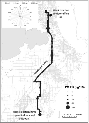
Figure 2. (a) Graph indicating the average particulate matter exposure by hour of the day for all combined personal samples. (b) Graph indicating the average PM_2.5 exposure overall, by location and by activity (with standard errors). Activity measurements were self-reported by participants in activity journals.

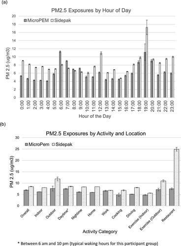
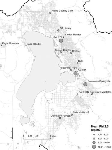
Figure 3. Map indicating the 15 sampling locations and their overall average PM_2.5 as measured by the SidePak over the course of the study period (µg/m³). The red star indicates the stationary monitor located in Lindon, UT. Daily data from this monitor are shown in Figure 5.

GPS tracking

We used a GPS tracker along with the personal exposure monitors for both personal and fixed-location sampling. This allowed us to pinpoint the locations at which measurements were being taken. We used a Bad Elf model BE-GPS-2200 GPS unit (Bad Elf LLC, West Hartford, CT), which was placed in the sampling vest. The unit recorded latitude and longitude coordinates that were downloaded as .kml files. GPS coordinates were matched with the MicroPEM measurements by time and date. As the GPS unit would not always collect readings indoors (due to impaired satellite connections), we used an algorithm identifying the closest GPS reading within 15 min of each MicroPEM sample to create a match. Those MicroPEM readings that did not have a GPS match within 15 min were not used in the personal calculations.

Outdoor air quality monitor

Daily PM_2.5 readings were obtained from an outdoor air pollution monitor located in Lindon, UT. The Lindon monitoring station is operated by the Utah Department of Environmental Quality (DEQ), Division of Air Quality, and collects continuous measures of PM_2.5, PM₁₀, wind speed, wind direction, and ambient temperature. Real-time PM_2.5 measures were collected using a tapered element oscillating microbalance (TEOM). The Lindon monitor was selected based on its centralized location in Utah County, and because it had complete outdoor air pollution data available for each 24-hr period during which personal and fixed-location samples were collected. The location of the monitoring station is shown in Figure 3 (shown later).

Instrument validation

After completion of all personal and fixed-location sampling, one MicroPEM and one SidePak were compared side-by-side to the Lindon air pollution monitor. The MicroPEM and SidePak were attached to a stand and placed on the roof of the Lindon air quality monitoring station within 18 inches of the TEOM air inlet. Instruments were run continuously for 5 hr 20 min during afternoon hours and the evening commute. Data points from the MicroPEM and SidePak were averaged over 6-min time intervals and time-matched to the Lindon monitor data, which also reported average PM_2.5 concentration in 6-min intervals. Instrument readings were compared using a mixed model analysis of variance (ANOVA) blocking on time. There was a significant effect by instrument on mean PM_2.5 concentration at the p < 0.05 level (F(2, 638) = 132.79, p < 0.0001). Post hoc comparisons were made using the Tukey–Kramer test. Results showed there was no difference between the Lindon monitor (M = 5.8 µg/m³, SD = 2.7) and the SidePak (M = 5.6 µg/m³, SD = 3.0) in mean PM_2.5 concentration (Difference = 0.2 µg/m³, T638 = 1.29, p = 0.40). However, there was a significant difference between the MicroPEM (M = 3.7 µg/m³, SD = 0.7) and both the Lindon monitor (Difference = 2.2 µg/m³, T638 = 14.72, p < 0.0001) and the SidePak (Difference = –2.0 µg/m³, T638 = –13.42, p < 0.0001). Based on these findings we determined that the Lindon monitor and SidePak instruments could be directly compared to each other, but not to the MicroPEM. We did not evaluate intra- or interinstrument bias. Based on manufacturers’ laboratory calibration procedures, intrainstrument variability can range to ±10% for both the SidePaks and MicroPEMs. However, instrument performance may vary under field-use conditions, and nephelometer data reported here might not reflect manufacturers’ reported precisions.

Pump flow rates were postcalibrated on all instruments following each participant and each day of fixed-location sampling. For personal exposure monitors, a pre- to postcalibration difference within ±5% was considered acceptable (DiNardi and AIHA, 2003). Postcalibration flow rates were within ±4.61% and ±4.37% of precalibration values for SidePaks and MicroPEMs, respectively. MicroPEM nephelometer zeroes were checked during postcalibration using Docking Station software. Instruments were turned on for at least 5 min with an in-line HEPA filter in place, after which the nephelometer reading was checked. All instrument nephelometers read zero at postcalibration. For the SidePaks, instruments were used with an alkaline battery pack. This increased sample collection times, but instruments were dead when returned to the laboratory. Thus, postcalibration flow rates were measured with new batteries installed in the instruments, which may have affected flow rates, and laser diode zeroes were not checked post sample collection. TSI reports the zero stability of the SidePak is ±1.0 µg/m³ over 24 hr.

To account for hygroscopic particle enlargement due to relative humidity (RH), MicroPEMs were operated with the RH correction factor enabled. However, over the sampling period RH averaged 36.9% (18.3–74.8%) and 32.7% (16.2–67.5%) as measured by personal and fixed-location MicroPEMs, respectively. At these low RH levels we would expect inappreciable hygroscopic particle growth, and no influence on the MicroPEM nephelometer (Williams, 2014). No corrections were made to the SidePak data.

Data alignment

Data from the MicroPEM, SidePak, GPS, and personal journals were joined using an algorithm that matched samples based on time. As described, for the personal samples we joined the MicroPEM data with the GPS readings based on the closed reading within 15 min. Since the fixed-location samples were entirely outdoors and the GPS never lost connection with the satellite, we matched GPS coordinates as the most recent reading within 3 min of a SidePak reading. The MicroPEMs did not show stable readings below 3 µg/m³, so time points that had a MicroPEM level below 3 were dropped to calculate averages by hour of day and activity. For the fixed-location monitoring, only SidePak measurements were used since they were compared to the Lindon monitor rather than the MicroPEM. The journals were also joined to the personal monitor readings using a time- and date-matching algorithm. Since the journals recorded each 15 min of personal activity, MicroPEM readings were simply assigned the activity category that was recorded for the 15-min time window during which they occurred.

Analysis

We computed the mean, standard error, and standard deviation PM_2.5 measures for each personal sample by time of day. We also calculated these measures combined for all samples. Average PM_2.5 exposure was calculated by activity as self-reported in participants’ journals. Activity-specific particulate concentrations were reported for total indoor and outdoor exposures and for indoor and outdoor locations separately. The activity subcategories reported were cooking, driving, eating at a restaurant, and exercising (indoors and outdoors).

Fixed-location sample measurements taken by the SidePak were combined by week and interpolated using empirical Bayesian Kriging as implemented in ArcMap v. 10.2 using an empirical data transformation. The transformation brought the data close to normal distribution, but with some variation from the line of normality on a QQ-plot at the tails. This was due to many weeks having a few locations with very low pollution exposures making transformation difficult. This, in combination with variability in sample timing, means that kriging results represent rough estimates. Measurements taken at the same location were averaged prior to interpolation. Bayesian Kriging repeatedly estimates the underlying semivariogram in order to account for uncertainty in the covariance functions (Pilz and Spock, 2008). Only readings within 0.15 miles of the central latitude and longitude point recorded in Table S1 were used, rather than all readings taken in between fixed-location monitoring stops. A range of 10–15 nearest neighbors was used to create prediction and standard error maps.

We reported the MicroPEM readings in the text with and without levels lower than 3 µg/m³. This is in line with known limitations in the instrument as described by the manufacturers at RTI. Due to necessary settings on the nephelometer, the MicroPEM records data at very low pollution levels in intervals of three. Leaving in the zero values would result in an underestimate of exposure, since background pollution levels are actually always greater than zero.

To estimate personal exposure for each participant using the fixed-location samples, individual paths were layered on top of the Kriged values from their corresponding week. Finally, the interpolated air pollution values were extracted for each GPS-recorded point and averaged to provide an estimated personal exposure with standard error (Figure S4). These estimates were compared with the true personal samples, as well as with average 24-hr PM_2.5 measurements from the Lindon air pollution monitor.

Results

Personal monitoring

There were in total 10 participants in the study who wore the MicroPEM and SidePak personal air pollution monitors for a 24-hr period. Each participant’s PM_2.5 exposure was mapped according to the person’s location and graphed by time of day. To protect confidentiality, individual maps are not shown here, except for an example participant who consented to having his or her location data mapped (Figure 1). However, individual graphs over time using the SidePak and MicroPEM measures are shown in Figures S2 and S3, respectively. Maps revealed variation in exposure levels, even while traveling along the same roadway.

Journals were returned to study personnel complete, aside from participant 8, who did not account for his or her activities between 10:00 a.m. and 3:00 p.m.; participant 1, who did not account for his or her activities between 10:00 a.m and 11:00 a.m.; and participant 10, who did not account for his or her activities between 5:30 a.m. and 10:00 a.m. Based on personal journals, participants spent an average of 86.9% of their time indoors and 10.2% of their time outdoors (2.9% of time not defined). Participants reported spending approximately half (47.5%) of their time in their home. Of those who reported working, 22.7% of their time was spent at work. More time was reportedly spent in restaurants than cooking, 0.5% (3 participants reporting activity) compared to 0.4% (2 participants reporting activity).

The average PM_2.5 exposure recorded by the MicroPEM nephelometer (without readings below 3 removed) was 2.4 µg/m³ (range = (0–4825 µg/m³), stderr = 0.06). Due to low indoor pollution levels, many participants had the bulk of their personal pollution readings as zero, for reasons described in the following. An average of 64% of data points were removed from individual data collection to report the average with readings below 3 removed. This increased average personal exposure levels to increase to 6.93 µg/m³ (stderr = 0.15). The true average is between the readings with zeros included and without. The average exposure recorded by the SidePak was higher (8.47 µg/m³, range = (0–4434 µg/m³), stderr = 0.10). Individual exposure varied widely by activity and time of day. PM_2.5 average levels according to the MicroPEM and SidePak are shown in Figure 2 for all participants by time, location, and activity.

All but three participants (P4, P7, and P8) had single time point exposure levels exceeding 100 µg/m³; however, we did not find any consistent time–activity patterns or exposure windows that explain these results. Based on diary entries, participants 1, 6, and 10 had short-term peak exposures > 100 µg/m³ during evening hours, corresponding to being at work, being near a campfire, and being at home, respectively. Participant 2 experienced a peak exposure around 3:00 p.m. and participant 5 around 11:00 a.m. (both at work). Participants 3, 9, and 10 had peak exposures after 10:00 p.m., when they reported being at home. Considering PM_2.5 originates primarily from fuel combustion, we postulate that these exposures may have come from domestic activities such as burning candles or cooking. As shown in Figure 2a, the highest average level by hour of day was between 7:00 p.m. and 7:59 p.m. (MicroPEM = 11.14 µg/m³, stderr = 2.05, SidePak = 17.23 µg/m³, stderr = 1.79), and the lowest was between 3:00 p.m. and 3:59 p.m. (MicroPEM = 4.47 µg/m³, stderr = 0.12, SidePak = 4.77 µg/m³, stderr = 0.08). Levels were also very low during the early morning hours (2–4 a.m.). During the peak window between 7:00 and 7:59 p.m., participants were exposed during commuting, eating in a restaurant, cooking at home, and participating in outdoor activities. Vehicle emissions were likely the primary source of exposure during commuting and evening outdoor activities, while frying, sautéing, or open-grill cooking may explain the home and restaurant exposures. There was a second, smaller window of elevated readings between 7 and 9 p.m. Note that a single participant (participant 6) was near a campfire at 7:35 p.m. (4,825 µg/m³ as measured by the MicroPEM). These readings are responsible for some of the larger standard errors seen between 7 and 9 p.m. This reading is shown in Figures S2 and S3. SidePak and MicroPEM readings were typically proportionate to each other, except for around 12:00 p.m. and 7:00 p.m. (SidePak higher).

Average particulate exposure was highest while participants were outdoors (MicroPEM = 7.61 µg/m³, stderr = 1.08, SidePak = 11.85 µg/m³, stderr = 0.83) or in restaurants (MicroPEM = 7.48 µg/m³, stderr = 0.39, SidePak = 24.93 µg/m³, stderr = 0.82), and lowest when participants were exercising indoors (MicroPEM = 4.78 µg/m³, stderr = 0.23, SidePak = 5.63 µg/m³, stderr = 0.08). Exposures while driving were comparatively high (MicroPEM = 5.13 µg/m³, stderr = 0.10, SidePak = 8.03 µg/m³, stderr = 0.09). The categories are not mutually exclusive. For example, exposures while exercising outdoors were also counted as part of the total outdoor exposure.

Fixed-location monitoring

Data collected from the 15 fixed-location monitoring sites with the SidePak were used to interpolate particulate levels for Utah County. Each site’s average particulate level for the entire study period is shown in Figure 3 and Table S1. The highest exposure levels on average were taken in downtown Springville in southern Utah county (12.38 µg/m³, stderr = 0.45), while the lowest levels were recorded at the Eagle Mountain sampling location (4.71 µg/m³, stderr = 0.13). As shown in Figure S4, however, areas of high and low particulate concentrations varied from week to week.

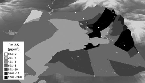
After the Bayesian Kriging of the SidePak data was completed for each week, individual participants’ paths were then mapped on top of the interpolated values, and average levels were extracted based on participants’ locations as described. Interpolated values for all of Utah County are shown in Figure 4, while values from individual weeks are shown in Figure S4 with prediction standard errors. The data shown in Figure 4 are collapsed data that were subject to temporal variability, and should be interpreted as a broad estimate of microclimate locations.

Figure 4. Map showing the overall data using Bayesian Kriging to interpolate values between sampling locations. Data are draped over a three-dimensional Utah elevation map. The location of sampling sites are shown as gray dots. The variation in PM_2.5 concentrations demonstrates the large variation in microclimates in Utah County. (Measurements are from SidePak. For maps by week, see Figure S4.)

The range of average PM_2.5 exposure levels estimated for each participant using the interpolated fixed-location data was 2.83 to 19.26 µg/m³ (mean = 8.3, stderr = 1.4). These estimated levels were compared with average exposure from personal samples (Figure 5). Data from the stationary outdoor monitor in Lindon, UT, were added for reference. As data between the Lindon monitor and SidePak were comparable, the SidePak data were used to estimate fixed-location measurements.

Figure 5. Graph showing comparisons in PM_2.5 estimates between personal breathing zone monitoring and estimated exposures from fixed-location sampling using the SidePak. Bars represent average 24-hr levels with standard errors. The line graph represents PM_2.5 values recorded at the Lindon, UT, outdoor stationary monitor, and is included for reference.

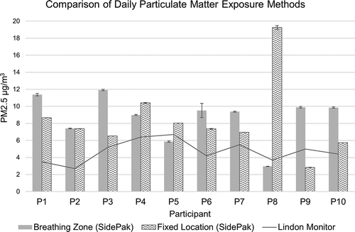
When comparing the personal samples with estimates from the interpolated fixed-location samples, 7 of 10 participants (except 5, 8, and 9) had personal exposure measures that were more closely approximated by the fixed-location method than by the central Lindon monitor. The Lindon monitor particulate measurements ranged from 2.7 µg/m³ to 6.7 µg/m³. Participant 8’s exposure was especially not well estimated using fixed-location monitoring. This participant spent a great deal of time traveling through and staying in high-pollution areas, but remained predominantly indoors.

Discussion

Outdoor stationary monitors have been the standard measurement equipment for estimating PM_2.5 levels for research and public health awareness for decades. There is tremendous interest in using GIS to accurately interpolate local exposure levels using stationary monitors, traffic-related data, and land use methods (Brauer et al., 2003; Hoek et al., 2008; Eeftens et al., 2012). These techniques are very sophisticated and would be improved with more precise results than stationary monitors alone. However, the development of personal exposure monitors provides valuable opportunities to collect even more precise information for governments and individuals. These new tools allow for less reliance on stationary monitors to identify pollution microclimates. Such data have the potential to be very powerful in studying the impacts of air pollution on human health while providing individuals with preexisting respiratory conditions the data they need to make informed decisions. We chose a sampling method that was very simple, and the analysis tools we chose are commonly available to government entities seeking to supplement measurement networks that are currently using stationary monitors alone. While temporal and spatial variability likely influenced our results in ways that make them not as reliable for more strict research purposes, they did still more closely approximate the gold standard of personal monitoring than a centralized monitor. The very broad range in personal exposure levels and microclimates shown in this study reinforces their utility for discerning local areas of high pollution and tracking individual exposure.

In our study, the highest exposure levels were outside, including those exposures that occurred while driving. Vehicle emissions and roadway exposures were major contributors to individual particulate exposures in Utah County. Restaurants represented the indoor activity with the highest levels of PM_2.5. The mean PM_2.5 exposure in our study (SidePak = 24.93 µg/m³) was similar to values reported by Brown et al. (2012) for restaurants during the summer (Brown et al., 2012). This was expected, since previous studies have identified cooking in large volume on open grills as a significant source of particulate matter exposure (Zhao et al., 2007; Abdullahi et al., 2013; Taner et al., 2013). Restaurant PM_2.5 exposures deserve further study because high particulate levels may represent an occupational health hazard to restaurant employees.

While the self-reported journals were very helpful in identifying time spent indoors and outdoors (including driving time), there are some activities for which the time spent and thus exposure levels were underestimated. The clearest example of this was cooking, which was only self-reported by two participants. Since the participants only recorded their own activities, they would not have reported another household member cooking despite the fact that they were still probably exposed to particulates from that activity.

Results from this study are consistent with previous research showing that particulate matter exposures measured in the breathing zone are generally higher than estimates from centralized outdoor air pollution monitors (Ozkaynak et al., 1995; Janssen et al., 1998; Meng et al., 2005; Rodes et al., 2010; Wallace et al., 2011; Wheeler et al., 2011; Bereznicki et al., 2012; Stevens et al., 2014). This difference is partially explained by individuals’ time–activity patterns as they travel through various microclimates during their daily activities. By measuring microclimate PM_2.5 levels throughout Utah County using the fixed-location monitoring strategy, we were able to more closely approximate participants’ breathing-zone exposures in 7 of 10 subjects compared to estimates from the stationary outdoor monitor. These findings suggest that GPS-enabled personal exposure monitors may have application in current air pollution monitoring programs.

This study was limited by a relatively small number of participants, and by short-duration sampling during one annual season. Air pollution levels are heavily influenced along the Wasatch front by season, with the highest PM_2.5 concentrations occurring during winter weather inversions (Pope, 1995). The microclimate exposures identified in this study may change dramatically during winter months. This study was also limited by PM_2.5 estimates from the MicroPEMs. Tracking of microclimate exposures requires data from real-time particle counters that can be compared to personal time–activity patterns. Personal exposures are usually based on measures from optical particle counters that use photometric light scattering to estimate airborne particulate matter concentrations. The light scattering properties of airborne particulate matter differ widely by location and pollution source, and for best results must be calibrated with an aerosol similar to the one being sampled. In this study, we did not collect enough particulate mass on the MicroPEM filters to compare nephelometer and gravimetric results. However, using a second personal monitor that was comparable with the central Lindon monitor was a strength, in that we were able to overcome some of the limitations of the MicroPEMs. For the SidePak instruments, we recognize that there may have been some particle loss due to the length of the Tygon tubing. Instrument accuracy may have also been affected by body/tube movement on the participant, which influenced pump flow rates.

As technology continues to improve the capability of personal monitors and to reduce cost, more research is needed into how to best integrate these monitors into personal health decision making and current government monitoring programs. Personal particulate monitors will become more accessible to individuals with underlying respiratory and cardiovascular conditions who want to monitor particulate levels in order to protect their own health. The data would certainly be valuable to government health offices, as having more detailed data on regional pollution microclimates can motivate policy changes toward reducing the burden of air pollution. We found that in comparing the two monitors, each had strengths and weaknesses. In conducting individual-level data collection, the MicroPEM is more practical in that it weighs much less than the SidePak and is far quieter. Many participants found the SidePak’s noise level bothersome. It also is able to collect both gravimetric and nepholometer-based results, and contains an accelerometer, making it a major step forward in personal sampling versatility. However, the MicroPEM pulls air at a low flow rate (making it very quiet, but collecting less dust than other monitors), and does not currently perform well at low pollution levels. This may improve as the technology advances. The SidePak performs well at a range of pollution levels and was shown to be comparable to the central monitoring site used in this study. However, it does not collect dust for gravimetric analysis. In government monitoring situations the SidePak may be very useful for collecting data to supplement those of central monitors if noise and weight are not an issue. Also, of note, with an extended battery pack the batteries can last about 22 hr in the SidePak, whereas they can last up to 40 hr in the MicroPEM.

In our study, we identified localized variation in PM_2.5 concentrations that served to more accurately estimate the exposure levels of individuals traveling through the environment than a central monitoring site alone. These estimates were not perfect, however, especially for those who traveled outside the measured area or participated in high-exposure activities. Government-level use of fixed-location sampling may be a good solution for using personal monitors to explore and identify local pollution microclimates. Individual-level monitoring may be better for those who either participate in high-risk activities or have underlying conditions.

Funding

The authors gratefully acknowledge the support of staff at the Utah Department of Environmental Quality, Division of Air Quality for the assistance with data from the Lindon stationary monitor and Ryan Chartier and Jonathan Thornburg at RTI International for technical assistance with the MicroPEMs. This work was funded by Brigham Young University.

Supplemental Data

Supplemental data for this paper can be accessed at the publisher’s website

Additional information

Funding

The authors gratefully acknowledge the support of staff at the Utah Department of Environmental Quality, Division of Air Quality for the assistance with data from the Lindon stationary monitor and Ryan Chartier and Jonathan Thornburg at RTI International for technical assistance with the MicroPEMs. This work was funded by Brigham Young University.

Notes on contributors

Chantel D. Sloan

Chantel D. Sloan, Tyler J. Philipp, Rebecca K. Bradshaw, Sara Chronister, W. Bradford Barber, and James D. Johnston work in the Department of Health Science at the Brigham Young University.

Tyler J. Philipp

Chantel D. Sloan, Tyler J. Philipp, Rebecca K. Bradshaw, Sara Chronister, W. Bradford Barber, and James D. Johnston work in the Department of Health Science at the Brigham Young University.

Rebecca K. Bradshaw

Chantel D. Sloan, Tyler J. Philipp, Rebecca K. Bradshaw, Sara Chronister, W. Bradford Barber, and James D. Johnston work in the Department of Health Science at the Brigham Young University.

Sara Chronister

Chantel D. Sloan, Tyler J. Philipp, Rebecca K. Bradshaw, Sara Chronister, W. Bradford Barber, and James D. Johnston work in the Department of Health Science at the Brigham Young University.

W. Bradford Barber

Chantel D. Sloan, Tyler J. Philipp, Rebecca K. Bradshaw, Sara Chronister, W. Bradford Barber, and James D. Johnston work in the Department of Health Science at the Brigham Young University.

James D. Johnston

Chantel D. Sloan, Tyler J. Philipp, Rebecca K. Bradshaw, Sara Chronister, W. Bradford Barber, and James D. Johnston work in the Department of Health Science at the Brigham Young University.

References

- Abdullahi, K.L., J.M. Delgado-Saborit, and R.M. Harrison 2013. Emissions and indoor concentrations of particulate matter and its specific chemical components from cooking: A review. Atmos. Environ. 71:260–94. doi:10.1016/j.atmosenv.2013.01.061
- Adams, H., M. Nieuwenhuijsen, R. Colvile, M. McMullen, and P. Khandelwal. 2001. Fine particle (PM 2.5) personal exposure levels in transport microenvironments, London, UK. Sci. Total Environ. 279(1):29–44. doi:10.1016/S0048-9697(01)00723-9
- Anderson, J.O., J.G. Thundiyil and A. Stolbach. 2012. Clearing the air: A review of the effects of particulate matter air pollution on human health. J. Med. Toxicol. 8(2):166–75. doi:10.1007/s13181-011-0203-1
- Avery, C.L., K.T. Mills, R. Williams, K.A. McGraw, C. Poole, R.L. Smith, and E.A. Whitsel. 2010. Estimating error in using residential outdoor PM2.5 concentrations as proxies for personal exposures: a meta-analysis. Environ. Health Perspect. 118(5):673. doi:10.1289/ehp.0901158
- Bereznicki, S.D., J.R. Sobus, A.F. Vette, M.A. Stiegel, and R.W. Williams. 2012. Assessing spatial and temporal variability of VOCs and PM-components in outdoor air during the Detroit Exposure and Aerosol Research Study (DEARS). Atmos. Environ. 61:159–68. doi:10.1016/j.atmosenv.2012.07.008
- Berrio, P., V. Sanchez, V. Tapia, G. Gonzalez, K. Steenland, R. Chartier, C. Rodes, L. Naeher, and O. Adetona. 2013. Assessment of exposure to wood combustion generated household air pollution in Ayacucho, Peru. Health 1(2):3.
- Brauer, M., G. Hoek, P. van Vliet, K. Meliefste, P. Fischer, U. Gehring, J. Heinrich, J. Cyrys, T. Bellander, M. Lewne, and B. Brunekreef. 2003. Estimating long-term average particulate air pollution concentrations: application of traffic indicators and geographic information systems. Epidemiology 14(2):228–39. doi:10.1097/01.EDE.0000041910.49046.9B
- Breen, M.S., T.C. Long, B.D. Schultz, J. Crooks, M. Breen, J.E. Langstaff, K.K. Isaacs, Y.-M. Tan, R.W. Williams, and Y. Cao. 2014. GPS-based microenvironment tracker (MicroTrac) model to estimate time–location of individuals for air pollution exposure assessments: Model evaluation in central North Carolina. J. Expos. Sci. Environ. Epidemiol. 24(4):412–20. doi:10.1038/jes.2014.13
- Brook, R.D., S. Rajagopalan, C.A. Pope, 3rd, J.R. Brook, A. Bhatnagar, A.V. Diez-Roux, F. Holguin, Y. Hong, R.V. Luepker, M.A. Mittleman, A. Peters, D. Siscovick, S.C. Smith, Jr., L. Whitsel, J.D. Kaufman, American Heart Association Council on Epidemiology and Prevention, Council on the Kidney in Cardiovascular Disease, and Council on Nutrition, Phyiscal Activity and Metabolism. 2010. Particulate matter air pollution and cardiovascular disease: An update to the scientific statement from the American Heart Association. Circulation 121(21):2331–78. doi:10.1161/CIR.0b013e3181dbece1
- Brown, K.W., J.A. Sarnat, and P. Koutrakis. 2012. Concentrations of PM2.5 mass and components in residential and non-residential indoor microenvironments: The Sources and Composition of Particulate Exposures study. J. Expos. Sci. Environ. Epidemiol. 22(2):161–72. doi:10.1038/jes.2011.41
- Dales, R., L. Liu, A.J. Wheeler, and N.L. Gilbert. 2008. Quality of indoor residential air and health. Can. Med. Assoc. J. 179(2):147–52. doi:10.1503/cmaj.070359
- Das, R., K. Allen, M. Morishita, B. Nan, B. Mukherjee, J. Harkema and J. Wagner. 2014. Cardiovascular depression during inhalation exposure to a mixture of ozone and rural ambient fine particles (PM2.5) in rats on a high fructose diet. Am. J. Respir. Crit. Care Med. 189:A1668.
- Dias, D., and O. Tchepel. 2014. Modelling of human exposure to air pollution in the urban environment: A GPS-based approach. Environ. Sci. Pollut. Res. 21(5):3558–71. doi:10.1007/s11356-013-2277-6
- DiNardi, S.R., and American Industrial Hygiene Association. 2003. The Occupational Environment: Its Evaluation, Control, and Management. Fairfax, VA: AIHA Press (American Industrial Hygiene Association).
- Dons, E., L. Int Panis, M. Van Poppel, J. Theunis, H. Willems, R. Torfs, and G. Wets. 2011. Impact of time–activity patterns on personal exposure to black carbon. Atmos. Environ. 45(21):3594–602. doi:10.1016/j.atmosenv.2011.03.064
- Dons, E., M. Van Poppel, B. Kochan, G. Wets and L. I. Panis. 2014. Implementation and validation of a modeling framework to assess personal exposure to black carbon. Environ. Int. 62: 64–71. doi:10.1016/j.envint.2013.10.003
- Eeftens, M., R. Beelen, K. de Hoogh, T. Bellander, G. Cesaroni, M. Cirach, C. Declercq, A. Dedele, E. Dons, A. de Nazelle, K. Dimakopoulou, K. Eriksen, G. Falq, P. Fischer, C. Galassi, R. Grazuleviciene, J. Heinrich, B. Hoffmann, M. Jerrett, D. Keidel, M. Korek, T. Lanki, S. Lindley, C. Madsen, A. Molter, G. Nador, M. Nieuwenhuijsen, M. Nonnemacher, X. Pedeli, O. Raaschou-Nielsen, E. Patelarou, U. Quass, A. Ranzi, C. Schindler, M. Stempfelet, E. Stephanou, D. Sugiri, M. Y. Tsai, T. Yli-Tuomi, M. J. Varro, D. Vienneau, S. von Klot, K. Wolf, B. Brunekreef, and G. Hoek. 2012. Development of land use regression models for PM2.5, PM2.5 absorbance, PM10 and PMcoarse in 20 European study areas; Results of the ESCAPE project. Environ. Sci. Technol. 46(20):11195–205.
- Eide, M., and D. Lillquist. The Occupational Environment: Its Evaluation, Control and Management. Fairfax, VA, AIHA Press.
- Fann, N., A.D. Lamson, S.C. Anenberg, K. Wesson, D. Risley and B.J. Hubbell. 2012. Estimating the national public health burden associated with exposure to ambient PM2.5 and ozone. Risk Anal. 32(1):81–95. doi:10.1111/j.1539-6924.2011.01630.x
- Gamble, J.F. 1998. PM2.5 and mortality in long-term prospective cohort studies: cause-effect or statistical associations? Environ. Health Perspect. 106(9):535–49. doi:10.1289/ehp.98106535
- Gerharz, L.E., O. Klemm, A.V. Broich, and E. Pebesma. 2013. Spatio-temporal modelling of individual exposure to air pollution and its uncertainty. Atmos. Environ. 64:56–65. doi:10.1016/j.atmosenv.2012.09.069
- Glad, J.A., L.L. Brink, E.O. Talbott, P.C. Lee, X.H. Xu, M. Saul, and J. Rager. 2012. The relationship of ambient ozone and PM2.5 levels and asthma emergency department visits: Possible influence of gender and ethnicity. Arch. Environ. Occup. Health 67(2):103–8. doi:10.1080/19338244.2011.598888
- Gu, J., U. Kraus, A. Schneider, R. Hampel, M. Pitz, S. Breitner, K. Wolf, O. Hänninen, A. Peters, and J. Cyrys. 2015. Personal day-time exposure to ultrafine particles in different microenvironments. Int. J. Hyg. Environ. Health 218(2):188–95. doi:10.1016/j.ijheh.2014.10.002
- Gulliver, J., and D.J. Briggs. 2004. Personal exposure to particulate air pollution in transport microenvironments. Atmos. Environ. 38(1):1–8. doi:10.1016/j.atmosenv.2003.09.036
- Hasenfratz, D., O. Saukh, S. Sturzenegger, and L. Thiele. 2012. Participatory air pollution monitoring using smartphones. Mobile Sensing. April 16–20, 2012.
- Hochstetler, H.A., M. Yermakov, T. Reponen, P.H. Ryan, and S.A. Grinshpun. 2011. Aerosol particles generated by diesel-powered school buses at urban schools as a source of children’s exposure. Atmos. Environ. 45(7):1444–53. doi:10.1016/j.atmosenv.2010.12.018
- Hoek, G., R. Beelen, K. de Hoogh, D. Vienneau, J. Gulliver, P. Fischer, and D. Briggs. 2008. A review of land-use regression models to assess spatial variation of outdoor air pollution. Atmos. Environ. 42(33):7561–78. doi:10.1016/j.atmosenv.2008.05.057
- Janssen, N.A.H., G. Hoek, B. Brunekreef, H. Harssema, I. Mensink, and A. Zuidhof. 1998. Personal sampling of particles in adults: Relation among personal, indoor, and outdoor air concentrations. Am. J. Epidemiol. 147(6):537–47. doi:10.1093/oxfordjournals.aje.a009485
- Klepeis, N.E., W.C. Nelson, W.R. Ott, J.P. Robinson, A.M. Tsang, P. Switzer, J.V. Behar, S.C. Hern, and W.H. Engelmann. 2001. The National Human Activity Pattern Survey (NHAPS): A resource for assessing exposure to environmental pollutants. J. Expos. Anal. Environ. Epidemiol. 11(3):231–52. doi:10.1038/sj.jea.7500165
- Lippmann, M. 2014. Toxicological and epidemiological studies of cardiovascular effects of ambient air fine particulate matter (PM2.5) and its chemical components: coherence and public health implications. Crit. Rev. Toxicol. 44(4):299–347. doi:10.3109/10408444.2013.861796
- Meng, Q.Y., B.J. Turpin, L. Korn, C.P. Weisel, M. Morandi, S. Colome, J.J. Zhang, T. Stock, D. Spektor, A. Winer, L. Zhang, J.H. Lee, R. Giovanetti, W. Cui, J. Kwon, S. Alimokhtari, D. Shendell, J. Jones, C. Farrar, and S. Maberti. 2005. Influence of ambient (outdoor) sources on residential indoor and personal PM2.5 concentrations: analyses of RIOPA data. J. Expos. Anal. Environ. Epidemiol. 15(1):17–28. doi:10.1038/sj.jea.7500378
- Miranda, M.L., S.E. Edwards, M.H. Keating, and C.J. Paul. 2011. Making the environmental justice grade: the relative burden of air pollution exposure in the United States. Int. J. Environ. Res. Public Health 8(6):1755–71. doi:10.3390/ijerph8061755
- Ozkaynak, H., J. Xue, J. Spengler, L. Wallace, E. Pellizzari and P. Jenkins. 1995. Personal exposure to airborne particles and metals: Results from the particle team study in Riverside, California. J. Expos. Anal. Environ. Epidemiol. 6(1):57–78. doi:10.1097/00001648-199503000-00239
- Pilz, J., and G. Spock. 2008. Why do we need and how should we implement Bayesian kriging methods. Stochast. Environ. Res. Risk Assess. 22(5):621–32. doi:10.1007/s00477-007-0165-7
- Pope, C. III. 1995. Particulate pollution and health: a review of the Utah valley experience. J. Expos. Anal. Environ. Epidemiol. 6(1):23–34. doi:10.1097/00001648-199503000-00237
- Pope, C. A. III. 1991. Respiratory hospital admissions associated with PM10 pollution in Utah, Salt Lake, and Cache Valleys. Arch. Environ. Health 46(2):90–97. doi:10.1080/00039896.1991.9937434
- Pope, C. A. III, J. Schwartz, and M.R. Ransom. 1992. Daily mortality and PM10 pollution in Utah Valley. Arch. Environ. Health 47(3):211–17. doi:10.1080/00039896.1992.9938351
- Rodes, C., S. Chillrud, W. Haskell, S. Intille, F. Albinali, and M. Rosenberger. 2012. Predicting adult pulmonary ventilation volume and wearing complianceby on-board accelerometry during personal level exposure assessments. Atmos. Environ. 57:126–37. doi:10.1016/j.atmosenv.2012.03.057
- Rodes, C.E., P.A. Lawless, J.W. Thornburg, R.W. Williams, and C.W. Croghan. 2010. DEARS particulate matter relationships for personal, indoor, outdoor, and central site settings for a general population. Atmos. Environ. 44(11):1386–99. doi:10.1016/j.atmosenv.2010.02.002
- Sloan, C.D., A.S. Andrew, J.F. Gruber, K.M. Mwenda, J.H. Moore, T. Onega, M.R. Karagas, X. Shi, and E.J. Duell. 2012. Indoor and outdoor air pollution and lung cancer in New Hampshire and Vermont. Toxicol. Environ. Chem. 94(3):605–15. doi:10.1080/02772248.2012.659930
- Sorensen, M., B. Daneshvar, M. Hansen, L.O. Dragsted, O. Hertel, L. Knudsen, and S. Loft. 2003. Personal PM2.5 exposure and markers of oxidative stress in blood. Environ. Health Perspect. 111(2):161–66. doi:10.1289/ehp.5646
- Steinle, S., S. Reis, and C. Sabel. 2011. Assessment of personal exposure to air pollutants in Scotland—An integrated approach using personal monitoring data. MODSIM. http://www.mssanz.org.au.previewdns.com/modsim2011/E1/steinle.pdf.
- Steinle, S., S. Reis, and C.E. Sabel. 2013. Quantifying human exposure to air pollution—Moving from static monitoring to spatio-temporally resolved personal exposure assessment. Sci. Total Environ. 443:184–93. doi:10.1016/j.scitotenv.2012.10.098
- Stern, G., P. Latzin, M. Roosli, O. Fuchs, E. Proietti, C. Kuehni, and U. Frey. 2013. A prospective study of the impact of air pollution on respiratory symptoms and infections in infants. Am. J. Respir. Crit. Care Med. 187(12):1341–48. doi:10.1164/rccm.201211-2008OC
- Stevens, C., R. Williams and P. Jones. 2014. Progress on understanding spatial and temporal variability of PM 2.5 and its components in the Detroit Exposure and Aerosol Research Study (DEARS). Environ. Sci. Processes Impacts 16(1):94–105. doi:10.1039/C3EM00364G
- Taner, S., B. Pekey, and H. Pekey. 2013. Fine particulate matter in the indoor air of barbeque restaurants: Elemental compositions, sources and health risks. Sci. Total Environ. 454–55:79–87. doi:10.1016/j.scitotenv.2013.03.018
- Wallace, L.A., A.J. Wheeler, J. Kearney, K. Van Ryswyk, H. You, R.H. Kulka, P.E. Rasmussen, J.R. Brook and X. Xu. 2011. Validation of continuous particle monitors for personal, indoor, and outdoor exposures. J. Expos. Sci. Environ. Epidemiol. 21(1):49–64. doi:10.1038/jes.2010.15
- Wheeler, A.J., X. Xu, R. Kulka, H. You, L. Wallace, G. Mallach, K.V. Ryswyk, M. MacNeill, J. Kearney, and P.E. Rasmussen. 2011. Windsor, Ontario exposure assessment study: Design and methods validation of personal, indoor, and outdoor air pollution monitoring. J. Air Waste Manage. Assoc. 61(2):142–56. doi:10.3155/1047-3289.61.2.142
- Wheeler, A.J., X. Xu, R. Kulka, H. You, L. Wallace, G. Mallach, K. Van Ryswyk, M. MacNeill, J. Kearney, and P.E. Rasmussen. 2011. Windsor, Ontario Exposure Assessment Study: Design and methods validation of personal, indoor, and outdoor air pollution monitoring. J. Air Waste Manage. Assoc. 61(3):324. doi:10.3155/1047-3289.61.3.324
- Williams, R., J. Suggs, A. Rea, K. Leovic, A. Vette, C. Croghan, L. Sheldon, C. Rodes, J. Thornburg, and A. Ejire. 2003. The Research Triangle Park particulate matter panel study: PM mass concentration relationships. Atmos. Environ. 37(38):5349–63. doi:10.1016/j.atmosenv.2003.09.019
- Williams, R.K., A. Kaufman, T. Hanley, J. Rice, and S. Garvey. 2014. Evaluation of field-deployed low cost PM sensors. Washington, DC: U.S. EPA. EPA/600/R-14/464.
- Zhao, Y. L., M. Hu, S. Slanina, and Y. H. Zhang. 2007. The molecular distribution of fine particulate organic matter emitted from Western-style fast food cooking. Atmos. Environ. 41(37):8163–8171. doi:10.1016/j.atmosenv.2007.06.029
- Zuurbier, M., G. Hoek, M. Oldenwening, V. Lenters, K. Meliefste, P. van den Haze, and B. Brunekreef. 2010. Commuters’ exposure to particulate matter air pollution is affected by mode of transport, fuel type, and route. Environ. Health Perspect. 118(6):783–89. doi:10.1289/ehp.0901622
- Zuurbier, M., G. Hoek, M. Oldenwening, K. Meliefste, P. van den Hazel, and B. Brunekreef. 2011. Respiratory effects of commuters’ exposure to air pollution in traffic. Epidemiology 22(2):219–27. doi:10.1097/EDE.0b013e3182093693