Source apportionment of emissions from light-duty gasoline vehicles and other sources in the United States for ozone and particulate matter

ABSTRACT

Federal Tier 3 motor vehicle emission and fuel sulfur standards have been promulgated in the United States to help attain air quality standards for ozone and PM_2.5 (particulate matter with an aerodynamic diameter <2.5 μm). The authors modeled a standard similar to Tier 3 (a hypothetical nationwide implementation of the California Low Emission Vehicle [LEV] III standards) and prior Tier 2 standards for on-road gasoline-fueled light-duty vehicles (gLDVs) to assess incremental air quality benefits in the United States (U.S.) and the relative contributions of gLDVs and other major source categories to ozone and PM_2.5 in 2030. Strengthening Tier 2 to a Tier 3-like (LEV III) standard reduces the summertime monthly mean of daily maximum 8-hr average (MDA8) ozone in the eastern U.S. by up to 1.5 ppb (or 2%) and the maximum MDA8 ozone by up to 3.4 ppb (or 3%). Reducing gasoline sulfur content from 30 to 10 ppm is responsible for up to 0.3 ppb of the improvement in the monthly mean ozone and up to 0.8 ppb of the improvement in maximum ozone. Across four major urban areas—Atlanta, Detroit, Philadelphia, and St. Louis—gLDV contributions range from 5% to 9% and 3% to 6% of the summertime mean MDA8 ozone under Tier 2 and Tier 3, respectively, and from 7% to 11% and 3% to 7% of the maximum MDA8 ozone under Tier 2 and Tier 3, respectively. Monthly mean 24-hr PM_2.5 decreases by up to 0.5 μg/m³ (or 3%) in the eastern U.S. from Tier 2 to Tier 3, with about 0.1 μg/m³ of the reduction due to the lower gasoline sulfur content. At the four urban areas under the Tier 3 program, gLDV emissions contribute 3.4–5.0% and 1.7–2.4% of the winter and summer mean 24-hr PM_2.5, respectively, and 3.8–4.6% and 1.5–2.0% of the mean 24-hr PM_2.5 on days with elevated PM_2.5 in winter and summer, respectively.

Implications: Following U.S. Tier 3 emissions and fuel sulfur standards for gasoline-fueled passenger cars and light trucks, these vehicles are expected to contribute less than 6% of the summertime mean daily maximum 8-hr ozone and less than 7% and 4% of the winter and summer mean 24-hr PM_2.5 in the eastern U.S. in 2030. On days with elevated ozone or PM_2.5 at four major urban areas, these vehicles contribute less than 7% of ozone and less than 5% of PM_2.5, with sources outside North America and U.S. area source emissions constituting some of the main contributors to ozone and PM_2.5, respectively.

Introduction

The U.S. Environmental Protection Agency (EPA) has set new “Tier 3” vehicle emission standards for tailpipe and evaporative emissions from passenger cars, light-duty trucks, medium-duty passenger vehicles, and some heavy-duty vehicles and lowered the allowed sulfur content of gasoline to approximately 10 ppm, considering the vehicle and its fuel as an integrated system (EPA, 2014a). The Tier 3 standards are closely coordinated with California’s Low Emission Vehicle (LEV III) standards. The primary aim of these standards is to improve ambient air quality, as emissions of volatile organic compounds (VOCs), nitrogen oxides (NO_x), and particulate matter (PM) from vehicles are often key precursors to ambient ozone (O₃) and fine particulate matter (aerodynamic diameter <2.5 μm; PM_2.5). The Tier 3 program is a successor to EPA’s Tier 2 federal emissions program, finalized in 2000, and the earlier Tier 1 program.

It is useful to understand the ambient air quality benefits of the Tier 3 emissions program as well as the likely major contributors to the residual ambient O₃ and PM_2.5 concentrations after implementation of the program. In a prior modeling study (Vijayaraghavan et al., 2012), we examined the incremental benefits of the Tier 1 and Tier 2 programs as well as nationwide adoption of a standard similar to the LEV III standards for on-road gasoline-fueled light-duty vehicles (gLDVs) for O₃ and PM_2.5 concentrations in the eastern United States (U.S.) in 2022. Gasoline sulfur was assumed to comply with a standard of 30 ppm sulfur except in California where the counties used lower sulfur, and the reductions in NO_x, VOCs, and sulfur dioxide (SO₂) emissions due to gasoline sulfur reductions mandated by the LEV III standard were not considered. Another limitation of the prior study was the lack of complete phase-in of the LEV III standard by 2022, the basis year for comparing emission standards. The current study builds upon the prior work by considering a more reasonable lower gasoline sulfur content and its effect on emissions, and considers a year further in the future (2030) when greater (70%) penetration of the LEV III (i.e., Tier 3) vehicle fleet is expected to occur. We also assess the relative contributions of various anthropogenic emission source categories in the U.S. and sources outside the U.S. to O₃ and PM_2.5 concentrations in 2030.

We apply state-of-the-science emissions models and an advanced regional three-dimensional (3-D) photochemical air quality model, the Comprehensive Air Quality Model with Extensions (CAMx) (ENVIRON, 2011), that simulates transport and dispersion, atmospheric chemical transformation, and deposition to the earth’s surface of trace gases and aerosols, along with the CAMx O₃ Source Apportionment Technology (OSAT) (Yarwood et al., 1996; Dunker et al., 2002) and Particulate Source Apportionment Technology (PSAT) (Yarwood et al., 2005) for source apportionment. OSAT uses multiple tracer species to track the fate of ozone precursor emissions (VOC and NO_x) and the ozone formation caused by these emissions within a simulation (ENVIRON, 2011). The tracers operate as spectators to the normal CAMx calculations so that the underlying CAMx predicted relationships between emission groups (sources) and ozone concentrations at specific locations are not perturbed. The tracers in the OSAT track the effects of chemical reaction, transport, diffusion, emissions, and deposition within CAMx and allow ozone formation from multiple “source groupings” to be tracked simultaneously, where the source grouping could be a region or source sector. Similarly, in PSAT, reactive tracers are added for each source category/region for primary PM and secondary PM and precursors. The OSAT and/or PSAT tools have been widely applied to estimate the contributions of multiple source areas and categories to O₃ and PM formation in the U.S., respectively (e.g., Wagstrom et al., 2008; Koo et al., 2009; EPA, 2010a; Collet et al., 2014b). Here, we apply CAMx with these tools to estimate the incremental benefits of the different gLDV emissions and fuel programs in 2030 and to assess the contributions of gLDVs and other sources O₃ and primary and secondary PM in the eastern U.S. in 2030 in hypothetical scenarios with the Tier 2 standard and nationwide LEV III standards with 30 and 10 ppm gasoline sulfur.

Methods

Modeling domain and emissions scenarios

The air quality simulations are conducted with CAMx using on-road emissions inventories derived using the Motor Vehicle Emission Simulator (MOVES) (EPA, 2010b) and other model inputs as discussed below. We applied version 5.40 of CAMx with the Carbon Bond 5 (CB05) chemical mechanism and version 2010a of MOVES.

The geographic region studied here follows that in Vijayaraghavan et al. (2012) and includes part of the eastern U.S. with focus on 4 of 13 urban areas discussed in EPA’s PM Risk Assessment analysis (EPA, 2010c). The four areas selected are Atlanta, Detroit, Philadelphia, and St. Louis. The CAMx modeling domain extends over the Continental U.S. (CONUS) at 36-km horizontal resolution, with an inner nested domain at 12-km resolution over part of the eastern U.S. including the four urban areas of interest (Figure 1). The domain has a pressure-based vertical structure with 26 layers, with the model top at 145 mb or approximately 14 km above mean sea level.

Figure 1. Air quality modeling domain and urban areas analyzed.

The model performance of this CAMx configuration was previously evaluated for a 2008 baseline year (Vijayaraghavan et al., 2012). The 2008 CAMx predictions of 1-hr and 8-hr average O₃ concentrations were compared with measurements in the Air Quality System (AQS) network (EPA, 2013) and the Clean Air Status and Trends Network (CASTNET; EPA, 2011a). Model predictions of PM_2.5 mass and components were compared with daily (24-hr) average measurements in the AQS and the Interagency Monitoring of Protected Visual Environments (IMPROVE, 1995) networks. Overall, model performance was good for O₃ in the eastern U.S., with mean normalized bias (MNB) for 8-hr O₃ ranging from 5.6% to 26.7% (depending on season and network) at over 500 monitoring stations, mean normalized error (MNE) ranging from 11.3% to 28.6%, and unpaired peak accuracy ranging from −11.9% to 28.4%, with some overprediction of summertime ozone. Model performance for 24-hr PM_2.5 was found comparable to previous studies (see Vijayaraghavan et al., 2012, and references cited therein), with mean fractional bias (MFB) ranging from −3.4% to 49.6% at over 140 monitoring stations and mean fractional gross error (MFE) ranging from 32.8% to 54.7%. The bias and error for 24-hr PM_2.5 mass and components were within the model performance criteria of Boylan and Russell (2006). More detailed information on the CAMx model performance evaluation may be found elsewhere (Vijayaraghavan et al., 2012).

Three 2030 LDV scenarios are modeled here:

1. 2030 Tier 2 with approximately 30 ppm gasoline sulfur (assume that only U.S. Tier 2 standards are implemented through 2030)

2. 2030 LEV III with approximately 30 ppm gasoline sulfur (assume that the California LEV III standard is adopted nationwide, i.e., similar to Tier 3 standard, but with 30 ppm sulfur)

3. 2030 LEV III with approximately 10 ppm gasoline sulfur (assume that the California LEV III standard is adopted nationwide, similar to Tier 3 standard with 10 ppm sulfur)

Emissions from all sources other than gLDVs are held constant across the three 2030 scenarios and calculated as described below. 2030 is chosen as the modeling year following EPA’s selection of 2030 as the future year in its Regulatory Impacts Analysis for the Tier 3 rulemaking; 70% of the vehicle miles traveled in 2030 are from vehicles that meet the fully phased-in Tier 3 standards (EPA, 2014b).

All simulations are conducted for a winter month (February) and summer month (July).

Meteorology

The air quality simulations with CAMx for the 2030 scenarios are driven by year 2008 meteorological fields from the Weather Research and Forecast (WRF) model–Advanced Research WRF (ARW) core (Skamarock et al., 2008). The WRF meteorological fields and performance evaluation are described elsewhere (Vijayaraghavan et al., 2012). The year 2008 was selected due to the availability of meteorological fields from the EPA (R. Gilliam, EPA, personal communication, 2011) and the availability of emissions from the National Emissions Inventory (NEI) used for the model performance evaluation in the prior study. The uncertainty associated with the choice of meteorological year is discussed later.

On-road motor vehicle emissions

The group of vehicle types collectively referred to as gLDVs includes three categories:

1. Light-duty gasoline vehicles (LDGV)

2. Light-duty gasoline trucks weighing less than 6000 lbs (LDGT1)

3. Light-duty gasoline trucks weighing between 6001 and 8500 lbs (LDGT2)

The Tier 2 program instituted gasoline sulfur and vehicle emission standards for nonmethane organic gases (NMOG), carbon monoxide (CO), NO_x, and PM for model years 2004 onwards and phased in completely in 2007 for the three categories of gLDVs considered in this study. The California LEV III standards apply to vehicle model years 2015–2028, with the phase-in for O₃ precursors, NO_x and NMOG, completed by 2025, and that for PM by 2028. The exhaust emission standards for the Tier 2 program, the California LEV III standards and the Federal Tier 3 program for gLDVs are shown in Tables 1, 2 and 3. The phase-in schedule for Tier 3 PM standards is shown in Table S1.1 (Supplemental Material). The main difference between the LEV III and Tier 3 standards is that the LEV III regulates PM down to a 1 mg/mi standard, whereas Tier 3 regulates it down to 3 mg/mi only. Thus, the current study, which applies the LEV III standard on a nationwide basis, simulates greater PM reduction than the Federal Tier 3 standard.

Table 1. Light-duty gasoline-vehicle exhaust emission standards^a,b (g/mi at 10 years/100,000 miles^c).

Standard	Model Year	NMOG	CO	NOx	PM	NMOG + NOx
Tier 2	2004+^d	0.0–0.09	0.0–4.2	0.07^e	0.0–0.02	—
LEV III	2015	—	—	—	—	0.100
	2016	—	—	—	—	0.093
	2017	—	—	—	0.006	0.086
	2018	—	—	—	0.005	0.079
	2019	—	—	—	0.004	0.072
	2020	—	—	—	0.003	0.065
	2021	—	—	—	0.003	0.058
	2022	—	—	—	0.003	0.051
	2023	—	—	—	0.003	0.044
	2024	—	—	—	0.003	0.037
	2025	—	—	—	0.0025	0.030
	2026	—	—	—	0.002	—
	2027	—	—	—	0.0015	—
	2028	—	—	—	0.001	—

Notes: NMOG = nonmethane organic gases; CO = carbon monoxide; NO_x = oxides of nitrogen; PM = particulate matter. ^aTier 2 data source: http://www.epa.gov/tier2/ (accessed February 2013). ^bLEV III data source: http://www.arb.ca.gov/msprog/levprog/leviii/meetings/071911/071911_lev_zev_eplabel_scoping.pdf (accessed January 2013). ^cExcept LEV III for which 150,000 mile standard is shown. ^d2004 to 2007 phase-in, ranges presented for all but NO_x emission rates due to phase-in with emission standards that vary by vehicle definition bin. ^eFleet-wide standard.

Table 2. Tier 3 LDV, LDT, and MDPV fleet average FTP NMOG + NO_x standards (mg/mi) (source: EPA, 2014a).

Vehicle Class	Model Year
	2017^a	2018	2019	2020	2021	2022	2023	2024	2025 and later
LDV/LDT1^b	86	79	72	65	58	51	44	37	30
LDT2, 3, and 4 and MDPV	101	92	83	74	65	56	47	38	30

Notes: FTP = Federal Test Procedure. ^bFor LDV and LDTs above 6000 lbs GVWR and MDPVs, the fleet average standards apply beginning in model year 2018. ^cThese standards apply for a 150,000 mile useful life. Manufacturers can choose to certify some or all of their LDVs and LDT1s to a useful life of 120,000 miles. If a vehicle model is certified to the shorter useful life, a proportionally lower numerical fleet average standard applies, calculated by multiplying the respective 150,000 mile standard by 0.85 and rounding to the nearest mg.

Table 3. Tier 3 LDV, LDT, and MDPV fleet average SFTP NMOG + NO_x standards (mg/mi) (source: EPA, 2014a).

Pollutant	Model Year
	2017^a	2018	2019	2020	2021	2022	2023	2024	2025 and later
NMOG + NOx	103	97	90	83	77	70	63	57	50

Notes: SFTP = Supplemental Federal Test Procedure. ^aFor LDVs and LDTs above 6000 lbs GVWR and MDPVs, the fleet average standards apply beginning in model year 2018.

MOVES 2010a is used to prepare on-road emissions inventories in the CONUS for the three 2030 emissions scenarios. MOVES is run for calendar year 2030 for vehicle aged 0–30 to develop on-road vehicle emissions for each scenario.

The emission factors complying with the LEV III or Tier 3 standards do not exist by default in MOVES and are simulated using alternative emissions inventory tools. Ratios of LEV III to LEV II emissions from the California Air Resources Board’s LEV III Inventory Database Tool (California Air Resources Board, 2011) are used to adjust MOVES model LEV II emission factors (EPA, 2010d) to calculate emission factors for the 2030 scenario of LEV III standards with approximately 30 ppm sulfur.

The 2010a version of MOVES includes the effect of low-sulfur gasoline (below 30 ppm) on exhaust emissions, but adjusts emissions via extrapolation from 30 ppm gasoline sulfur data collected from vehicles less modern than Tier 2. For this study, we improve upon the MOVES method by modeling the gasoline fuel sulfur effect using the California Predictive Model (California Air Resources Board, 2012). Exhaust emissions ratios from gasoline LDVs operating on ~10 ppm sulfur gasoline over ~30 ppm sulfur gasoline are used to adjust the emissions from the LEV III with ~30 ppm sulfur gasoline scenario to generate the LEV III with ~10 ppm sulfur gasoline scenario. The low-sulfur gasoline effects on emissions are estimated not only for gLDVs but all gasoline-fueled vehicle classes, including motorcycles and heavy-duty gasoline vehicles. Detailed information on the calculation of the on-road emissions in the three 2030 scenarios is provided in Supplemental Material (Section S2). A comparison of the on-road emissions results from the current study with those of the EPA Tier 3 rulemaking analysis for 2030 is also presented in Supplemental Material (Section S3).

CAMx-ready emissions are prepared from MOVES outputs following methods described earlier (Vijayaraghavan et al., 2012). The on-road emissions for winter and summer from MOVES for the three emissions scenarios are speciated to CAMx model species, spatially allocated to grid cells, and temporally allocated to hourly emissions using version 2.7 of the Sparse Matrix Operator Kernel Emissions (SMOKE) model (http://cmascenter.org/smoke). Emission estimates for total VOC are converted to the CB05 chemical mechanism in CAMx using VOC speciation profiles derived from EPA’s SPECIATE database, version 4.3 (EPA, 2011b). PM emissions are speciated to primary organic aerosol, primary elemental carbon, primary nitrate, primary sulfate, primary fine other PM, and coarse PM following methods outlined by Baek and DenBleyker (2010). On-road mobile sources generated using MOVES at the county level are allocated to CAMx 36-km and 12-km grid cells using spatial surrogates derived with the Spatial Surrogate Tool (http://www.epa.gov/ttn/chief/emch/spatial/spatialsurrogate.html).

Other emissions

Emissions from anthropogenic area and point sources in the CONUS other than on-road emissions for the 2030 emissions scenarios are compiled from the EPA 2030 inventory developed for the modeling analysis of the Heavy Duty Vehicle Green House Gas (HDGHG) Rule with emissions projected by EPA from 2005 data (EPA, 2011c). The source sectors obtained from the 2030 HDGHG inventory include fugitive dust, agricultural, nonpoint, electric generating units (EGUs), point sources other than EGUs, aircraft, locomotives, commercial marine vehicles, and nonroad sources. We used the projections by EPA for 2020 for anthropogenic area and point emissions for Canada and Mexico (EPA, 2010e) because these sources are not projected to 2030 in the EPA 2030 HDGHG modeling platform. The model simulations applied biogenic emissions of CO, nitric oxide, isoprene, and other VOCs, wildfire emissions of CO, NO_x, VOCs, sulfur dioxide (SO₂), ammonia (NH₃), and PM and sea salt emissions of particulate sodium, chloride, and sulfate developed previously (Vijayaraghavan et al., 2012) across the CAMx 36-km domain and are held constant across the emissions scenarios. All emissions inventories described above are converted to speciated, gridded, temporally varying emissions files suitable for air quality modeling with CAMx in the nested 36/12-km domains and are held constant across the three 2030 scenarios.

Other model inputs

Boundary concentrations of O₃, PM components and precursors, landuse/landcover data, and photolysis rates were obtained from the prior study (Vijayaraghavan et al., 2012) and held constant across the 2030 scenarios. In particular, boundary concentrations of O₃ and PM components and precursors for February and July 2008 (in addition to a 15-day model spin-up in each case) for the CAMx 36-km domain were derived from the global chemical and transport model, Model for Ozone and Related Chemical Tracers (MOZART) version 4.6 (Emmons et al., 2010), which applied 2008 meteorology driven by the Goddard Earth Observing System Model version 5 (GEOS-5; http://gmao.gsfc.nasa.gov/GEOS/) and global emissions inventory compiled during the Arctic Research of the Composition of the Troposphere from Aircraft and Satellites (ARCTAS) project (http://bio.cgrer.uiowa.edu/arctas/emission.html). Six-hourly model outputs in a latitude-longitude coordinate system with a spatial resolution of about 2.8° for both latitude and longitude and 28 vertical layers were mapped onto the CAMx domain and speciated for the CB05 chemical mechanism.

Emission sources and other categories for source attribution

Tracers are added in the OSAT tool in CAMx to track O₃ formation from O₃ precursors from the source categories shown in Table 4. These include anthropogenic and natural sources in the U.S., sources in Canada and Mexico, as well as the contribution of sources outside North America through boundary conditions for the 36-km grid resolution domain, referred to here as the North American background. The PSAT algorithm is similarly applied to track PM and precursors from these source categories.

Table 4. Source categories for source attribution.

Category	Description
S1	Area sources, i.e., nonpoint sources
S2	Nonroad mobile sources (“Nonroad”)
S3	On-road gasoline-fueled light-duty vehicles (“OnroadLDV”)
S4	Other on-road vehicles (“Onroad other”)
S5	Electric generating units (EGUs)
S6	Point sources other than EGUs (“nonEGU Pt”)
S7	Sources in Canada and Mexico in 36-km domain (“nonUS within 36 km domain”)
S8	Natural/biogenic emissions (“Natural”)
S9	Boundary conditions of 36-km domain (“North American background”)

Results and discussion

Emissions

In general, the gLDV emissions of VOC, NO_x, PM_2.5, CO, and SO₂ respond similarly in the four urban areas to the shift from Tier 2 to adoption of the LEV III standards and lower sulfur gasoline (Tables 5 and 6). However, the emission benefits are most pronounced in Detroit. The emission reductions from adopting LEV III emission standards with 10 ppm sulfur gasoline (i.e., percent change from Tier 2 to LEV III with 10 ppm S) are larger on a relative basis in Detroit than the other cities and the national total because Detroit’s gasoline LDV fleet is modeled using a younger fleet age distribution, resulting in LEV III vehicles making up a larger portion of the LDV fleet (i.e., it has more LDVs of the newer model years, including those that are affected by LEV III [2015+] than the fleets from other cities). When considering emissions from all on-road vehicles for an average winter and summer day (Tables 7 and 8), the NO_x benefit in Detroit due to the Tier 3-like standards is not distinctly larger than in the other areas because NO_x emissions from heavy-duty vehicles are not reduced in the LEV III scenario in any of the urban areas.

Table 5. Emissions from gasoline-fueled LDVs, winter 2030.

Region	Tier 2 30 ppm S (Mg day^−1)	LEV III 30 ppm S (Mg day^−1)	LEV III 10 ppm S (Mg day^−1)	Tier 2 − LEV III with 10 ppm S (Mg day^−1)	Tier 2 − LEV III with 10 ppm S(%)
VOC
CONUS	1919	1240	1219	700	−36%
Atlanta	28	18	18	10	−36%
Detroit	28	17	16	12	−42%
Philadelphia	18	11	11	7	−38%
NOx
CONUS	2096	1402	1269	827	−39%
Atlanta	32	21	19	13	−41%
Detroit	30	18	16	14	−47%
Philadelphia	16	11	10	7	−41%
PM2.5
CONUS	203	131	131	72	−35%
Atlanta	3	2	2	1	−31%
Detroit	4	2	2	2	−42%
CO
CONUS	62,567	43,980	43,395	19,172	−31%
SO2
CONUS	44	44	16	28	−63%

Table 6. Emissions from gasoline-fueled LDVs, summer 2030.

Region	LDV Tier 2 Emissions, ~30 ppm S (Mg day^−1)	LDV LEV III Emissions, ~30 ppm S (Mg day^−1)	LDV LEV III Emissions, ~10 ppm S (Mg day^−1)	Reduction from Tier 2 to LEV III with ~10 ppm S (Mg day^−1)	% Change from Tier 2 to LEV III with ~10 ppm
VOC
CONUS	1965	1220	1204	761	−39%
Atlanta	29	18	18	11	−38%
Detroit	27	15	15	12	−45%
Philadelphia	18	11	10	7	−40%
St. Louis	18	12	12	7	−37%
NOx
CONUS	2220	1495	1363	857	−39%
Atlanta	36	24	21	15	−41%
Detroit	28	16	15	13	−47%
Philadelphia	16	11	10	6	−40%
St. Louis	23	15	14	9	−39%
PM2.5
CONUS	117	89	89	28	−24%
Atlanta	2	2	2	0	−22%
Detroit	2	1	1	0	−24%
Philadelphia	1	1	1	0	− 21%
St. Louis	1	1	1	0	−24%
CO
CONUS	35,149	25,252	24,949	10,200	−29%
Atlanta	521	375	370	151	−29%
Detroit	424	288	284	140	−33%
Philadelphia	291	205	202	88	−30%
St. Louis	317	231	228	89	−28%
SO2
CONUS	51	51	18	32	−64%
Atlanta	1	1	0	1	−67%
Detroit	1	1	0	1	−67%
Philadelphia	1	1	0	0	−67%
St. Louis	1	1	0	0	−67%

Table 7. Emissions from all on-road vehicles, winter 2030.

Region	LDV Tier 2 Emissions, 30 ppm S (Mg day^−1)	LDV LEV III Emissions, 30 ppm S (Mg day^−1)	LDV LEV III Emissions,10 ppm S (Mg day^−1)	Reduction from Tier 2 to LEV III with 10 ppm S (Mg day^−1)	% Change from Tier 2 to LEV III with 10 ppm
VOC
CONUS	2439	1760	1736	703	−29%
Atlanta	34	24	24	10	−30%
Detroit	35	24	23	12	−34%
Philadelphia	24	18	18	7	−28%
St. Louis	24	18	18	6	−26%
NOx
CONUS	4851	4157	3988	863	−18%
Atlanta	73	62	59	14	−19%
Detroit	70	57	55	15	−21%
Philadelphia	33	28	26	7	−21%
St. Louis	57	50	48	9	−15%
PM2.5
CONUS	260	189	189	72	−27%
Atlanta	4	3	3	1	−23%
Detroit	5	4	4	2	−32%
Philadelphia	3	2	2	1	−28%
St. Louis	3	2	2	1	−27%
CO
CONUS	70,671	52,084	51,423	19,248	−27%
Atlanta	877	653	643	234	−27%
Detroit	1930	1338	1321	609	−32%
Philadelphia	755	542	534	221	−29%
St. Louis	615	465	459	156	−25%
SO2
CONUS	56	56	26	30	−53%
Atlanta	1	1	0	1	−55%
Detroit	1	1	0	0	−54%
Philadelphia	1	1	0	0	−60%
St. Louis	1	1	0	0	−55%

Table 8. Emissions from all on-road vehicles, summer 2030.

Region	LDV Tier 2 Emissions, 30 ppm S (Mg day^−1)	LDV LEV III Emissions, 30 ppm S (Mg day^−1)	LDV LEV III Emissions,10 ppm S (Mg day^−1)	Reduction from Tier 2 to LEV III with 10 ppm S (Mg day^−1)	% Change from Tier 2 to LEV III with 10 ppm S
VOC
CONUS	2694	1949	1931	763	−28%
Atlanta	36	25	25	11	−31%
Detroit	36	25	24	12	−33%
Philadelphia	27	20	20	7	−26%
St. Louis	27	20	20	7	−25%
NOx
CONUS	4738	4013	3848	890	−19%
Atlanta	74	61	59	15	−20%
Detroit	64	53	50	14	−21%
Philadelphia	31	26	25	6	−21%
St. Louis	54	47	45	9	−17%
PM2.5
CONUS	178	150	150	28	−16%
Atlanta	3	3	3	0	−14%
Detroit	3	3	3	0	−14%
Philadelphia	2	1	1	0	−15%
St. Louis	2	2	2	0	−14%
CO
CONUS	40,843	30,946	30,598	10,245	−25%
Atlanta	603	457	451	152	−25%
Detroit	513	376	372	141	−28%
Philadelphia	339	253	250	89	−26%
St. Louis	384	299	295	89	−23%
SO2
CONUS	65	65	31	34	−53%
Atlanta	1	1	1	1	−54%
Detroit	1	1	1	1	−54%
Philadelphia	1	1	0	0	−59%
St. Louis	1	1	0	0	−54%

If emission standards and gasoline sulfur regulations were to remain at the Tier 2 level with 30 ppm sulfur, the average 2030 VOC emissions from gLDVs during winter are approximately 1,900 Mg per day and slightly higher in summer. The adoption of more stringent LEV III emission controls with 30 ppm sulfur gasoline reduces the total on-road VOC emissions in the CONUS by 28% in both summer and winter relative to the Tier 2 case. The additional VOC benefit of switching to ~10 ppm sulfur gasoline (i.e., a standard similar to Tier 3) is 1%. The total CONUS NO_x emissions from gLDVs in Tier 2 with ~30 ppm sulfur gasoline are approximately 2,000 Mg per day on an average winter day and slightly higher in summer. The nationwide adoption of LEV III with ~30 ppm sulfur gasoline is estimated to reduce CONUS total on-road NO_x by 15%, and the reduction in gasoline sulfur to a 10 ppm standard reduces NO_x by another 4%. The total NO_x reduction is 19%, comparing the most stringent scenario (LEV III with 10 ppm sulfur standard gasoline) with the Tier 2 scenario.

NO_x emissions are higher in summer because higher running exhaust in summer more than compensate for higher cold start emissions in winter; more vehicle miles traveled (VMT) in summer results in more fuel consumed and higher NO_x exhaust emissions. In particular, Atlanta has the highest LDV emissions of NO_x, VOC, and PM_2.5 among the urban areas in summer due to a combination of higher ambient temperatures and higher VMT. SO₂ is higher in summer in all urban areas due to higher VMT. CO is higher in winter due to more frequent cold starts resulting from lower temperatures. Also, the higher average temperatures in summer result in more air-conditioning in vehicles, and that is accounted for in MOVES. The use of air-conditioning systems increases VOCs, CO, and NO_x emissions, but cold starts affect primarily CO (and VOCs to a lesser extent).

PM_2.5 emissions from gLDVs in the Tier 2 scenario are 74% higher for the average winter day compared with summer due to cold temperature effects on gasoline-vehicle PM exhaust. The gLDVs accounted for 78% and 66% of the total on-road PM_2.5 emissions during winter and summer, respectively. However, the on-road PM_2.5 emissions represent a very small fraction of total anthropogenic PM_2.5 inventory (see below). Compared with the Tier 2 scenario, the LEV III with ~10 ppm sulfur case reduces the gasoline LDV PM_2.5 emissions by 35% in winter and 24% in summer, and the CONUS total on-road PM_2.5 emissions by 27% and 16% in winter and summer, respectively.

Figure 2 presents the total anthropogenic emissions estimated in the CONUS and the fractions of the major source categories in February and July 2030 with a nationwide LEV III standard with 10 ppm gasoline sulfur. Similar plots are shown in Supplemental Material for the Tier 2 program and with a nationwide LEV III standard with 30 ppm sulfur (Figures S4.1 and S4.2). The sectors shown include area sources (comprising residential, commercial, and small industrial sources), EGUs, stationary point sources other than EGUs (abbreviated here as non-EGU Pt), off-road sources, gLDVs and other on-road sources. Following the implementation of the LEV III standard, NO_x emissions from gLDVs in 2030 represent 6% of the total CONUS anthropogenic inventory, reduced from 20% in 2008 (Vijayaraghavan et al., 2012) and 9% in 2030 with the Tier 2 standard (Supplemental Material). NO_x emissions from all on-road vehicles constitute approximately 18% of the total with the LEV III standard. Emissions from EGUs and point sources other than EGUs constitute the two largest NO_x source categories in the U.S. in 2030, each representing approximately 22% of the 2030 inventory.

Figure 2. Estimated wintertime and summertime anthropogenic emissions in the continental U.S. in 2030 with a nationwide LEV III standard with 10 ppm gasoline sulfur (Tier 3-like standard).

The on-road fraction of the anthropogenic inventory varies considerably across pollutants; it is highest for CO (28–49%), lower for VOCs (7%), and negligible for SO₂ (0.2%). CO emissions are dominated by on-road vehicles in winter but by off-road sources in summer (48% of total CO inventory). The doubling of off-road CO emissions from winter to summer is due to the sharp increase in usage in summer of the major nonroad emission sources: lawn and garden equipment and commercial equipment. Due to their slow reactivity, CO emissions have a much smaller effect on O₃ concentrations than NO_x or VOC emissions. NH₃ emissions from gLDVs constitute a large fraction (85%) of total on-road emissions but represent a very small fraction (2%) of the total anthropogenic inventory due to the dominance of other sources such as livestock farming. Although primary PM_2.5 emissions from vehicles can directly affect ambient PM_2.5, these represent a very small fraction (2–3%) of the total anthropogenic inventory; there is a much larger PM contribution from stationary sources, road dust, wood-burning, and other sources.

Ambient air quality

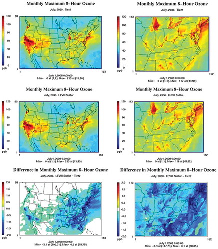
If LDV emission standards in 2030 were no more stringent than the Tier 2 standard, the summertime monthly mean of the MDA8 O₃ could be as high as 76 ppb over the eastern U.S. (near Washington, DC), with values exceeding 60 ppb in large parts of the eastern U.S. and the New York/New Jersey/Washington, DC, corridor experiencing more than 70 ppb (Figure 3). When considering the entire CONUS, the monthly mean goes up to 88 ppb, with the highest value predicted in the Los Angeles basin. The incremental benefits of the nationwide LEV III standards are examined by difference with the Tier 2 scenario (Figure 3; here “LEVIII” denotes the 30 ppm scenario and “LEVIIISulfur” denotes the 10 ppm scenario). Strengthening the Tier 2 standard to the Tier 3-like standard (LEV III with 10 ppm sulfur limit) results in a reduction of approximately 1 ppb in the monthly mean of MDA8 ozone in large parts of the eastern U.S. and up to 1.5 ppb (a 2.1% reduction from a maximum concentration of 70 ppb) near New York City. Reducing the gasoline sulfur limit from approximately 30 to 10 ppm reduces the monthly mean of MDA8 O₃ by up to 0.3 ppb in parts of the eastern U.S. (Figure S5.1). The monthly maximum of MDA8 O₃ with the Tier 3-like standard (Figure 4) exceeds 75 ppb in large parts of the eastern U.S., including Connecticut, Maryland, Pennsylvania, New Jersey, and New York City). Concentrations exceeding 75 ppb were also modeled by Collet et al. (2014a) in comparable regions in the eastern U.S. in a 2030 modeling study with a different air quality model, the Community Multiscale Air Quality Model (CMAQ). We find that the maximum reduction in the monthly maximum of MDA8 O₃ in the eastern U.S. is 2.8 ppb (or 2.7% from a concentration of 105 ppb near Washington, DC) from Tier 2 to the LEV III scenario with 30 ppm sulfur and by up to an additional 0.6 ppb (a 3.3% overall reduction from Tier 2) with the lower 10 ppm limit.

Figure 3. Monthly mean of daily maximum 8-hr ozone concentrations in July 2030 in the 36-km domain (left) and 12-km domain (right) in the Tier 2 scenario (top), “LEV III with 30 ppm sulfur” − Tier 2 (middle), and “LEV III with 10 ppm sulfur” − Tier 2 (bottom).

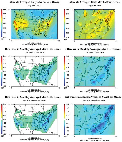
Figure 4. Monthly maximum of daily maximum 8-hr ozone concentrations in July 2030 in the 36-km domain (left) and 12-km domain (right) in the Tier 2 scenario (top), LEV III with 10 ppm sulfur scenario (middle), and “LEV III with 10 ppm sulfur” − Tier 2 (bottom).

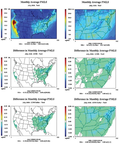
Wintertime monthly mean concentrations of PM_2.5 mass in the 2030 Tier 2 scenario exceed 15 μg/m³ (the annual mean standard for PM_2.5) in large parts of the Upper Midwest, Georgia, North Carolina, and the Northeast (Figure 5). The monthly mean decreases by up to 0.4 μg/m³ (a 2.7% reduction) in the LEV III 30 ppm scenario and by less than 0.1 μg/m³ additionally (a 3.3% overall reduction from Tier 2) with the lower 10 ppm standard (Figure S5.2). Reductions in PM_2.5 concentrations between the Tier 2 and LEV III scenarios are generally lower in summer (Figure 6) than winter, a maximum improvement of 0.2 μg/m³ in winter versus 0.4 μg/m³ in winter. This is likely due, in part, to less formation of PM nitrate from NO_x emissions in summer due to enhanced volatilization from the particulate phase (Vijayaraghavan et al., 2012). The exceptionally high summertime PM_2.5 concentrations predicted in northern California (>100 μg/m³) are due to emissions from extreme wildfire events in this region. Improvements in PM_2.5 are negligible in switching from 30 to 10 ppm sulfur except for some small reductions (0.04 μg/m³) in the Northeast (Figure S5.3).

Figure 5. Monthly mean of 24-hr PM_2.5 concentrations in February 2030 in the 36-km domain (left) and 12-km domain (right) in the Tier 2 scenario (top), “LEV III with 30 ppm sulfur” − Tier 2 (middle), and “LEV III with 10 ppm sulfur” − Tier 2 (bottom).

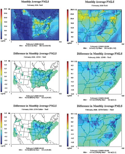
Figure 6. Monthly mean of 24-hr PM_2.5 concentrations in July 2030 in the 36-km domain (left) and 12-km domain (right) in the Tier 2 scenario (top), “LEV III with 30 ppm sulfur” − Tier 2 (middle), and “LEV III with 10 ppm sulfur” − Tier 2 (bottom).

Ozone and PM_2.5 source apportionment

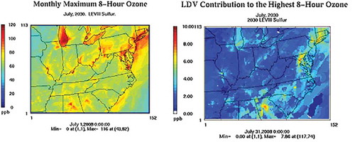
The OSAT tool in CAMx is used to track the ozone contribution from different emission groups with emphasis on the gLDVs. The summertime gLDV contributions to the monthly averaged MDA8 O₃ in 2030 under the Tier 2 program are highest in New York City, Atlanta, and Washington, DC, each averaging approximately 6 ppb O₃ (Figure 7), or approximately 9.4% (Figure S5.4). The LEV III program with 30 ppm sulfur results in reductions in gLDV contributions of approximately 1.8 ppb in the regions with the highest contributions in Tier 2. Additional reductions in the gLDV contribution with a 10 ppm sulfur limit are much smaller, less than 0.4 ppb throughout the domain. Overall, gLDVs in the LEV III scenario with 10 ppm sulfur contribute less than 5.5% to the monthly averaged MDA8 O₃ in most of the eastern U.S. (Figure S5.4), with the peak contribution of 6.1% near Atlanta. Ozone attainment will likely be influenced more by emission source contributions on days with elevated ozone concentrations. When considering the monthly highest MDA8 O₃, gLDV contributions range from 0 to 5 ppb across most of the eastern U.S. (Figure 8), with a peak absolute contribution of 7.9 ppb near Washington, DC, and a peak relative contribution of 10% (not shown) near Raleigh in North Carolina.

Figure 7. Contribution of gLDVs to the monthly mean of daily maximum 8-hr ozone in July 2030 in three scenarios: Tier 2 (top left), LEV III with 30 ppm sulfur (top middle), LEV III with 10 ppm sulfur (top right), “LEV III with 30 ppm sulfur” − Tier 2 (bottom middle), “LEV III with 10 ppm sulfur” − “LEV III with 30 ppm sulfur” (bottom right).

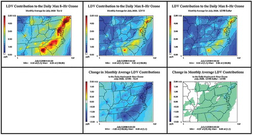
Figure 8. Monthly maximum of daily maximum 8-hr ozone concentrations in July 2030 in the LEV III 10 ppm sulfur scenario (left) and contribution of gLDVs to the maximum ozone concentration (right).

Figure 9 presents the relative contributions from the eight emission categories (listed in Table 4) and the North American background (boundary conditions) to the summertime monthly mean of MDA8 O₃ in Atlanta and Detroit in 2030. Similar plots are shown in Figure S5.5 for Philadelphia and St. Louis. Under the Tier 2 scenario, gLDVs are predicted to contribute 5 to 6% of the summertime mean MDA8 O₃ in Detroit, Philadelphia, and St. Louis, with the contribution higher in Atlanta at 9%. Under the Tier 3-like standard (the LEV III scenario with 10 ppm sulfur), the on-road LDV contributions to summertime mean MDA8 O₃ are reduced to 3–6%, whereas the North American background contributes 28–39% to the summertime mean O₃ across these four urban areas (or approximately 19–20 ppb in each area). The contribution of gLDVs to the monthly highest MDA8 O₃ (Figures 10 and S5.6) ranges from 6% to 11% under Tier 2 at the four urban areas. The Tier 3 emissions and fuel sulfur standards are effective in reducing the gLDV contribution to 3–7% of the highest MDA8 O₃ across these four areas. Interestingly, the share of the North American background to O₃ at Detroit drops from 39% to 19% when considering the day with highest ozone in July rather than the monthly mean, with that share picked up now by non-EGU point sources, EGUs, and natural sources.

Figure 9. Source apportionment of monthly mean of daily maximum 8-hr ozone in July 2030 in Tier 2 (left) and LEV III 10 ppm sulfur scenario (right) in Atlanta (top) and Detroit (bottom).

Figure 10. Source apportionment of monthly maximum of daily maximum 8-hr ozone in July 2030 in Tier 2 (left) and LEV III 10 ppm sulfur scenario (right) in Atlanta (top) and Detroit (bottom).

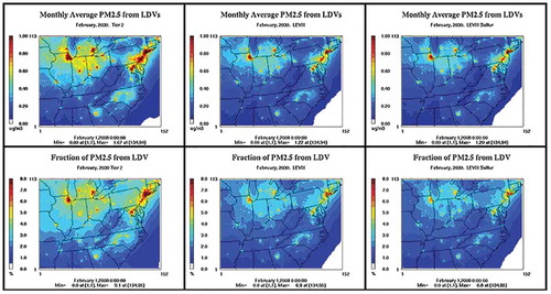
The gLDV contribution to monthly mean PM_2.5 is higher in February than in July (Figures 11 and S5.7) in all three scenarios due, in part, to higher gLDV primary PM_2.5 emissions arising from colder temperatures in winter. Under the Tier 2 scenario, the wintertime gLDV contributions are highest in urban areas in the upper Midwest and between Washington, DC, and New York City, with a peak contribution of 1.7 μg/m³ (or 9% of the total PM_2.5). LDV contributions in the southeastern U.S. are generally smaller than in the Northeast. The wintertime gLDV contribution is lower by between 0.3 and 0.4 μg/m³ in the LEV III 30 ppm scenario compared with the Tier 2 scenario in New York City, Chicago, and Detroit, representing 2% reductions in each region. Further strengthening of the standard to 10 ppm sulfur offered little additional PM_2.5 reductions in the 12-km domain. The largest PM_2.5 benefit going from Tier 2 to the LEV III with 30 ppm sulfur scenario (0.4 μg/m³) is an order of magnitude greater than the largest benefit (0.04 μg/m³) when transitioning from LEV III with 30 ppm sulfur to 10 ppm sulfur. This follows the smaller reduction in PM_2.5 precursor emissions with the transition from 30 to 10 ppm sulfur compared with the transition from Tier 2 to LEV III with 30 ppm sulfur. In July, gLDVs account for up to 4.3% of the total PM_2.5 under the Tier 2 program; the highest contribution is 0.6 μg/m³ in New York City. The LEV III program with 30 ppm sulfur reduces the PM_2.5 contribution up to 0.12 μg/m³; lowering the gasoline sulfur content to 10 ppm decreases the mean July contribution by less than 0.02 μg/m³.

Figure 11. Contribution of gLDVs to monthly average PM_2.5 in February 2030. Absolute contribution in μg/m³ (top) and relative contribution in % (bottom): Tier 2 (left), LEV III with 30 ppm sulfur (middle), and LEV III with 10 ppm sulfur (right).

Figures 12 and S5.8 present relative source contributions to the wintertime monthly mean of 24-hr PM_2.5 in Atlanta, Detroit, Philadelphia, and St. Louis in 2030. Similar plots are shown for summertime in Figures 13 and S5.9. Area source emissions (i.e., nonpoint sources) are the largest contributor to monthly averaged PM_2.5 in both winter and summer in all four urban areas in both scenarios, constituting 29–45% of the total PM_2.5, followed by non-EGU point sources in Detroit, Philadelphia, and St. Louis. Natural sources contribute over a third to mean summertime PM_2.5 in Atlanta, likely reflecting the influence of biogenic emissions in the region. On-road gLDVs account for 5–7% of the total PM_2.5 in February under Tier 2 controls, with the highest relative contribution in Detroit. As explained above, Detroit experiences a larger percent reduction in emissions from Tier 2 to LEV III compared with other three urban areas. LEV III controls with 30 ppm sulfur reduced the LDV impact by 2% in Detroit and 1% elsewhere from Tier 2 controls. Lowering the gasoline sulfur to 10 ppm offered little additional improvement for PM_2.5. In July, area, other, and non-EGU point sources are the largest contributors to PM_2.5 at these four cities. LDV contributions amounted to 2–3% of the total PM_2.5 under Tier 2 controls, and 2% under the LEV III scenarios at all four sites.

Figure 12. Source apportionment of monthly average 24-hr PM_2.5 in February 2030 in Tier 2 (left) and LEV III 10 ppm sulfur scenario (right) in Atlanta (top) and Detroit (bottom).

Figure 13. Source apportionment of monthly average 24-hr PM_2.5 in July 2030 in Tier 2 (left) and LEV III 10 ppm sulfur scenario (right) in Atlanta (top) and Detroit (bottom).

To investigate whether gLDVs have a larger contribution to days with elevated PM_2.5 than the monthly mean PM_2.5, we identified days with higher PM_2.5 (defined here as those with 24-hr PM_2.5 exceeding 15 μg/m³) and calculated average contributions from each source sector across those days. The threshold of 15 μg/m³ is somewhat arbitrary and is chosen to account roughly for the top 20–30% of days in each month for 24-hr PM_2.5. The results of this source apportionment at the four urban areas are presented in Figures 14, 15, S5.10, and S5.11. When considering days with elevated PM_2.5 only, the relative contribution of gLDVs to 24-hr PM_2.5 in winter and summer in the four urban areas ranges from 2% to 7% under Tier 2 and reducing to 1–5% under the Tier 3-like standard, and in both cases about 0.2% higher than when considering just the monthly mean PM_2.5. Area source emissions continue to be the dominant contributor to PM_2.5 in all four areas. A synopsis of the gLDV contributions to elevated ozone and PM_2.5 under the Tier 3-like standard in presented in Table 9.

Table 9. Contributions of gLDVs to elevated ozone and PM_2.5 concentrations in 2030 under the Tier 3-like standards (LEV III with 10 ppm sulfur).

	Atlanta		Detroit		Philadelphia		St. Louis
Measurement	Total	gLDV Contribution	Total	gLDV Contribution	Total	gLDV Contribution	Total	gLDV Contribution
Maximum daily 8-hr maximum ozone in July (ppb)	85.9	6.9%	74.9	3.1%	94.3	4.0%	86.6	3.7%
Average PM2.5 across days in February with 24-hr PM2.5 more than 15 μg/m^3 (μg/m^3)	18.3	4.0%	23.2	4.6%	26.0	4.5%	22.1	3.8%
Average PM2.5 across days in July with 24-hr PM2.5 more than 15 μg/m^3 (μg/m^3)	17.9	1.8%	17.9	2.0%	17.4	2.0%	16.3	1.5%

Figure 14. Source apportionment on days with elevated 24-hr PM_2.5 in February 2030 in Tier 2 (left) and LEV III 10 ppm sulfur scenario (right) in Atlanta (top) and Detroit (bottom): Average across days where the 24-hr PM_2.5 exceeds 15 μg/m³.

Figure 15. Source apportionment on days with elevated 24-hr PM_2.5 in July 2030 in Tier 2 (left) and LEV III 10 ppm sulfur scenario (right) in Atlanta (top) and Detroit (bottom): Average across days where the 24-hr PM_2.5 exceeds 15 μg/m³.

In summary, emissions from gLDVs contribute up to 6.1% to summertime monthly averaged MDA8 O₃ in the eastern U.S. following the nationwide implementation of a LEV III program with 10 ppm gasoline sulfur content similar to the Tier 3 standards, decreasing from 9.4% under the previous federal Tier 2 program. The North American background (global background concentrations) could constitute up to a third or more of U.S. ozone. PM precursor emissions from gLDVs in the eastern U.S. contribute up to 6.8% and 3.6% to winter and summer mean PM_2.5, respectively, under Tier 3-like standards, decreasing from 9.1% and 4.3%, respectively, under Tier 2, with area source emissions typically contributing over 30% in both programs. At the four urban areas of Atlanta, Detroit, Philadelphia, and St. Louis, gLDV emissions are responsible for up to 5.8% of the mean summertime MDA8 ozone and up to 5.0% of winter/summer mean 24-hr PM_2.5 concentrations under the Tier 3 program. When considering only days with higher O₃ and PM_2.5 concentrations under the Tier 3-like standards, gLDVs contribute up to 6.9% of summertime maximum MDA8 ozone and up to 4.6% to elevated winter/summer 24-hr PM_2.5 concentrations across these four areas. Thus, although gLDVs have a slightly (1%) higher contribution to peak O₃ compared with the monthly average, their relative contribution to PM_2.5 is lower when considering days with higher PM_2.5 instead of the monthly average, suggesting that those days are influenced more by other sources.

There is uncertainty in ozone and PM predictions associated with the choice of 2008 as the meteorological year. Weather-adjusted trend analyses of ambient concentrations in the U.S. by EPA (2015) shows that 2008 is neither particularly conducive nor nonconducive to ozone formation in the eastern U.S. The years 2005, 2007, 2010, and 2012 were more conducive to ozone formation in the Northeast than 2008, whereas the years 2003, 2004, 2006, and 2009 were less conducive than 2008 (see figures 2–5 in EPA, 2015). Thus, applying ambient air temperature and other meteorological fields from the former set of years would have likely resulted in greater local anthropogenic contributions (including those from on-road mobile sources) to ozone formation, whereas the converse would be true if meteorology from the latter set of years had been applied in modeling. Similarly, the choice of meteorological year also affects the prediction of the relative contributions of PM, in particular, that of secondary PM from local precursor sources of VOCs and NO_x such as on-road LDVs.

The CAMx OSAT and PSAT techniques provide a useful means to explore relative source contributions to ambient ozone and PM_2.5 concentrations. The application of these techniques here enables the estimation of the contribution of gasoline-fueled LDVs to residual ambient air pollution in the U.S. in 2030 following the implementation of the Tier 3 emissions and fuel sulfur standards.

Funding

This work was supported by the Coordinating Research Council Atmospheric Impacts Committee under Project A-76-3.

Supplemental Material

Supplemental data for this article can be accessed on the publisher’s website.

Additional information

Funding

This work was supported by the Coordinating Research Council Atmospheric Impacts Committee under Project A-76-3.

Notes on contributors

Krish Vijayaraghavan

Krish Vijayaraghavan and Chris Lindhjem are senior managers, Tejas Shah and Bonyoung Koo are managers, Edward Tai and Yesica Alvarez are associates, and Greg Yarwood is a principal at Ramboll Environ US Corporation, Novato, CA, USA. Allison DenBleyker is a staff engineer at Eastern Research Group, Boston, MA, USA.

Chris Lindhjem

Krish Vijayaraghavan and Chris Lindhjem are senior managers, Tejas Shah and Bonyoung Koo are managers, Edward Tai and Yesica Alvarez are associates, and Greg Yarwood is a principal at Ramboll Environ US Corporation, Novato, CA, USA. Allison DenBleyker is a staff engineer at Eastern Research Group, Boston, MA, USA.

Bonyoung Koo

Krish Vijayaraghavan and Chris Lindhjem are senior managers, Tejas Shah and Bonyoung Koo are managers, Edward Tai and Yesica Alvarez are associates, and Greg Yarwood is a principal at Ramboll Environ US Corporation, Novato, CA, USA. Allison DenBleyker is a staff engineer at Eastern Research Group, Boston, MA, USA.

Allison DenBleyker

Krish Vijayaraghavan and Chris Lindhjem are senior managers, Tejas Shah and Bonyoung Koo are managers, Edward Tai and Yesica Alvarez are associates, and Greg Yarwood is a principal at Ramboll Environ US Corporation, Novato, CA, USA. Allison DenBleyker is a staff engineer at Eastern Research Group, Boston, MA, USA.

Edward Tai

Krish Vijayaraghavan and Chris Lindhjem are senior managers, Tejas Shah and Bonyoung Koo are managers, Edward Tai and Yesica Alvarez are associates, and Greg Yarwood is a principal at Ramboll Environ US Corporation, Novato, CA, USA. Allison DenBleyker is a staff engineer at Eastern Research Group, Boston, MA, USA.

Tejas Shah

Krish Vijayaraghavan and Chris Lindhjem are senior managers, Tejas Shah and Bonyoung Koo are managers, Edward Tai and Yesica Alvarez are associates, and Greg Yarwood is a principal at Ramboll Environ US Corporation, Novato, CA, USA. Allison DenBleyker is a staff engineer at Eastern Research Group, Boston, MA, USA.

Yesica Alvarez

Krish Vijayaraghavan and Chris Lindhjem are senior managers, Tejas Shah and Bonyoung Koo are managers, Edward Tai and Yesica Alvarez are associates, and Greg Yarwood is a principal at Ramboll Environ US Corporation, Novato, CA, USA. Allison DenBleyker is a staff engineer at Eastern Research Group, Boston, MA, USA.

Greg Yarwood

Krish Vijayaraghavan and Chris Lindhjem are senior managers, Tejas Shah and Bonyoung Koo are managers, Edward Tai and Yesica Alvarez are associates, and Greg Yarwood is a principal at Ramboll Environ US Corporation, Novato, CA, USA. Allison DenBleyker is a staff engineer at Eastern Research Group, Boston, MA, USA.

References

- Baek, B.H., and A. DenBleyker. 2010. User’s Guide for the SMOKE-MOVES Integration Tool. Prepared for the U.S. Environmental Protection Agency Office of Air Quality Planning and Standards. July. http://cmascenter.org/smoke/documentation/smoke_moves_tool/SMOKE-MOVES_Tool_Users_Guide.pdf (accessed April 2013).
- Boylan, J.W., and A.G. Russell. 2006. PM and light extinction model performance metrics, goals, and criteria for three-dimensional air quality models. Atmos. Environ. 40:4946–4959. doi:10.1016/j.atmosenv.2005.09.087
- California Air Resources Board. 2011. LEV 3 Inventory Database Tool version 9h. November. http://www.arb.ca.gov/msprog/clean_cars/clean_cars_ab1085/lev3-inv-dbase_v9h.accdb (accessed April 2013).
- California Air Resources Board. 2012. Predictive model spreadsheets containing 2011 amendments. http://www.arb.ca.gov/fuels/gasoline/premodel/premodel.htm# (accessed January 2013).
- Collet, S., H. Minoura, T. Kidokoro, Y. Sonoda, Y. Kinugasa, and P. Karamchandani. 2014a. Evaluation of light-duty vehicle mobile source regulations on ozone concentration trends in 2018 and 2030 in the western and eastern United States. J Air Waste Manage. Assoc. 64:175–183. doi:10.1080/10962247.2013.845621
- Collet, S., H. Minoura, T. Kidokoro, Y. Sonoda, Y. Kinugasa, P. Karamchandani, J. Johnson, T. Shah, J. Jung, and A. DenBleyker. 2014b. Future year ozone source attribution modeling studies for the eastern and western United States. J Air Waste Manage. Assoc. 64:1174–1185. doi:10.1080/10962247.2014.936629
- Dunker A.M., G. Yarwood, J.P. Ortmann, and G.M. Wilson. 2002. Comparison of source apportionment and source sensitivity of ozone in a three dimensional air quality model. Environ. Sci. Technol. 36:29532964. doi:10.1021/es011418f
- Emmons, L.K., S. Walters, P.G. Hess, J.-F. Lamarque, G.G. Pfister, D. Fillmore, C. Granier, A. Guenther, D. Kinnison, T. Laepple, et al. 2010. Description and evaluation of the Model for Ozone and Related chemical Tracers, version 4 (MOZART-4). Geosci. Model Dev. 3:43–67. doi:10.5194/gmd-3-43-2010
- ENVIRON. 2011. User’s Guide, Comprehensive Air Quality Model with Extensions (CAMx), Version 5.40. http://www.camx.com (accessed August 2013).
- IMPROVE. 1995. IMPROVE Data Guide. University of California Davis, August 1995. http://vista.cira.colostate.edu/improve/Publications/OtherDocs/IMPROVEDataGuide/IMPROVEDataGuide.htm (accessed August 2013).
- U.S. Environmental Protection Agency. 2010a. Regulatory Impact Analysis for the Proposed Transport Rule. Docket ID No. EPA-HQ-OAR-2009-0491. Washington, DC: Office of Air Quality and Planning Standards, U.S. Environmental Protection Agency. July. http://www.epa.gov/ttn/ecas/regdata/RIAs/proposaltrria_final.pdf (accessed May 2013).
- U.S. Environmental Protection Agency. 2010b. Technical Guidance on the Use of MOVES2010 for Emission Inventory Preparation in State Implementation Plans and Transportation Conformity. EPA-420-B-10-023. Washington, DC: Office of Transportation and Air Quality, U.S. Environmental Protection Agency. April. http://www.epa.gov/otaq/models/moves/420b10023.pdf (accessed June 2013).
- U.S. Environmental Protection Agency. 2010c. Quantitative Health Risk Assessment for Particulate Matter. EPA-452/R-10-005. Washington, DC: Office of Air Quality Planning and Standards, U.S. Environmental Protection Agency. June. http://www.epa.gov/ttn/naaqs/standards/pm/data/PM_RA_FINAL_June_2010.pdf (accessed June 2013).
- U.S. Environmental Protection Agency. 2010d. LEV and Early NLEV modeling information. August. http://www.epa.gov/otaq/models/moves/MOVES2010a/levandearlynlevmodelinginformation.zip (accessed June 2013).
- U.S. Environmental Protection Agency. 2010e. 2020 Emissions Data from EPA’s 2005-Based v4 Modeling Platform. Prepared by Rich Mason, Office of Air Quality Planning and Standards, U.S. Environmental Protection Agency. April 15. ftp://ftp.epa.gov/EmisInventory/2005v4/2020emis/readme_2020_2005v4cap_bafm.doc (accessed July 2013).
- U.S. Environmental Protection Agency. 2011a. CASTNET. Clean Air Status and Trends Network. http://epa.gov/castnet/ (accessed July 2013).
- U.S. Environmental Protection Agency. 2011b. SPECIATE 4.3: Addendum to SPECIATE 4.2. Speciation Database Development Documentation. EPA/600/R-11/121. Prepared for the Office of Research and Development, U.S. Environmental Protection Agency. Prepared by TransSystems, E.H. Pechan & Associates. September. http://www.epa.gov/ttn/chief/software/speciate/speciate4/addendum4.2.pdf (accessed July 2013).
- U.S. Environmental Protection Agency. 2011c. Heavy-Duty Vehicle Greenhouse Gas (HDGHG) Emissions Inventory for Air Quality Modeling Technical Support Document. EPA-420-R-11-008. Washington, DC: Office of Air and Radiation, U.S. Environmental Protection Agency. August. http://www.epa.gov/otaq/climate/documents/420r11008.pdf (accessed July 2013).
- U.S. Environmental Protection Agency. 2013. Air Quality System User’s Guide Version 1.0.0. U.S. Environmental Protection Agency, Technology Transfer Network. July 31. http://www.epa.gov/ttn/airs/airsaqs/manuals/docs/users_guide.html (accessed November 2013).
- U.S. Environmental Protection Agency. 2014a. Control of Air Pollution from Motor Vehicles: Tier 3 Motor Vehicle Emission and Fuel Standards. Final Rule. Research Triangle Park, NC: U.S. Environmental Protection Agency. April. http://www.gpo.gov/fdsys/pkg/FR-2014-04-28/pdf/2014-06954.pdf (accessed April 2014).
- U.S. Environmental Protection Agency. 2014b. Control of Air Pollution from Motor Vehicles: Tier 3 Motor Vehicle Emission and Fuel Standards Final Rule. Regulatory Impacts Analysis. EPA-420-R-14-005. Washington, DC: U.S. Environmental Protection Agency. February. http://www.epa.gov/otaq/documents/Tier 3/420r14005.pdf (accessed March 2014).
- U.S. Environmental Protection Agency. 2015. Air Quality Modeling Technical Support Document for the 2008 Ozone NAAQS Transport Assessment. Office of Air Quality Planning and Standards, U.S. Environmental Protection Agency. January. http://www.epa.gov/airtransport/O3TransportAQModelingTSD.pdf (accessed August 2015).
- Vijayaraghavan, K., C. Lindhjem, A. DenBleyker, U. Nopmongcol, J. Grant, E. Tai, and G. Yarwood. 2012. Effects of light duty gasoline vehicle emission standards in the United States on O3 and particulate matter. Atmos. Environ. 60:109–120. doi:10.1016/j.atmosenv.2012.05.049
- Yarwood, G., R.E. Morris, M.A. Yocke, H. Hogo, and T. Chico. 1996. Development of a methodology for source apportionment of ozone concentration estimates from a photochemical grid model. Presented at the 89th Air & Waste Management Association Annual Meeting, Nashville, TN, June 23–28.