
ABSTRACT
A new method has been developed for a direct and remote measurement of industrial flare combustion efficiency (CE). The method is based on a unique hyper-spectral or multi-spectral Infrared (IR) imager which provides a high frame rate, high spectral selectivity and high spatial resolution. The method can be deployed for short-term flare studies or for permanent installation providing real-time continuous flare CE monitoring.
In addition to the measurement of CE, the method also provides a measurement for level of smoke in the flare flame regardless of day or night. The measurements of both CE and smoke level provide the flare operator with a real-time tool to achieve “incipient smoke point” and optimize flare performance.
The feasibility of this method was first demonstrated in a bench scale test. The method was recently tested on full scale flares along with extractive sampling methods to validate the method. The full scale test included three types of flares – steam assisted, air assisted, and pressure assisted. Thirty-nine test runs were performed covering a CE range of approximately 60-100%. The results from the new method showed a strong agreement with the extractive methods (r2=0.9856 and average difference in CE measurement=0.5%).
Implications: Because industrial flares are operated in the open atmosphere, direct measurement of flare combustion efficiency (CE) has been a long-standing technological challenge. Currently flare operators do not have feedback in terms of flare CE and smoke level, and it is extremely difficult for them to optimize flare performance and reduce emissions. The new method reported in this paper could provide flare operators with real-time data for CE and smoke level so that flare operations can be optimized. In light of EPA’s focus on flare emissions and its new rules to reduce emissions from flares, this policy-relevant development in flare CE monitoring is brought to the attention of both the regulating and regulated communities.
Introduction
Industrial flares are widely used primarily as safety devices in chemical process industries (e.g., petroleum refineries, chemical plants, etc.) and oil and gas fields. Waste process gases, particularly gases released due to process upset or emergency, are vented to flares to be safely combusted over the flare tips, avoiding industrial accidents and reducing air pollution. Although comprehensive emission inventories of flares and their associated emissions are not readily available, some anecdotal information is available to provide a sense of scale for the emission of volatile organic compounds (VOC) and greenhouse gases (GHG) from flares due to imperfect combustion. In the Fact Sheet for the Proposed Petroleum Refinery Sector Risk and Technology Review and New Source Performance Standards, the U.S. Environmental Protection Agency (EPA) states that the proposed new standards for flares will reduce VOC emissions from flares in this sector by 33,000 tons per year (EPA, 2014). In the same Fact Sheet, the total VOC emission reductions for all affected sources in this proposed rule are projected to be 52,000 tons per year. The flare portion accounts for 63% of the total reductions. There are more flares in chemical and petrochemical sectors. In 2007, the Texas Commission on Environmental Quality (TCEQ) conducted a special emission inventory of Highly Reactive Volatile Organic Compounds (HRVOC) in Harris County for the period from February 1, 2006 to January 31, 2007. HRVOC is a subset of VOC that represents the most potent ozone precursors. Results of this special emission inventory showed that the HRVOC emissions from flares were 1,469.5 tons out of a total HRVOC emission inventory of 2,433.4 tons in Harris County, Texas; that is, flare emissions accounted for 60.8% of total HRVOC emissions (ENVIRON, Citation2008).
Emissions from flares also represent a significant contribution to GHG emissions. According to a report by GE Energy, approximately 150 billion cubic meters of natural gas are flared in the world each year, roughly the same as the annual household consumption for the entire United States. The flaring of 150 billion cubic meters of natural gas produces 400 million tons per year of carbon dioxide (CO2), equivalent to annual emissions from 77 million cars (34% of the U.S. fleet) (Farina, Citation2011). The GHG impact for 1 lb of methane emissions is equivalent to 21 lb of CO2 emissions. Since the amount of methane emission is a function of flare combustion efficiency (CE), estimation of CE for these flares has a large impact on these GHG emission estimates.
Current practice is to assume that flares control 98% of the hydrocarbons (largely VOC) fed to flares, provided that some surrogate parameters (e.g., heat content of the vent gases and exit velocity of gases at the flare tip) are within established ranges. Field studies and modeling analyses conducted in Texas (e.g., Texas Air Quality Study of 2000, and Texas Air Quality Study II in 2006) have demonstrated that these assumptions regarding flare CE may be inaccurate, and total flare emissions in this airshed could be significantly underestimated. The uncertainty introduced into emission inventories due to flare CE assumptions could be significant enough to alter the outcome of large-scale air quality management decision making. Despite its importance, determining flare CE (and therefore emission rates) remains a technological challenge. Unlike other emission sources, the combustion for an industrial flare occurs in open air, leaving no practical method for capturing postcombustion gases. As a result, it is not possible to routinely apply traditional methods (such as extractive sampling) for analysis of the postcombustion gases or determination of control efficiency. Flare operations typically involve a drastic “turn-down ratio,” that is, changes in the volume of gases sent to flares in a very short period of time when an upset or emergency release occurs. The sharp changes in throughput can significantly disrupt the proper steam or air to fuel ratio and therefore alter flare efficiency. Due to these factors, determination of flare CE and destruction and removal efficiency (DRE) is extremely difficult. In 2009, TCEQ contracted with the University of Texas Austin (UT) to conduct a comprehensive study on flare CE and DRE (Allen and Torres, Citation2011). Results from this study (hereafter referred to the TECQ 2010 flare study) are very valuable in characterizing flare CE and DRE under the test conditions, and they have had a lasting impact on flare operations and flare management programs. One of the findings demonstrated that even if a flare is operated in accordance with the federal regulation 40 CFR §60.18, it still may not achieve assumed 98% CE. A reduction in CE from 98% to 90% represents a fivefold increase in flare emissions.
While the TCEQ 2010 flare study was a major undertaking, it demonstrated that realistic operating conditions can result in a large variability in flare CE. In many cases flare operators do have the means to optimize flare operating conditions (e.g., changing the steam to vent gas ratio, adding supplemental fuel, etc.). However, their ability to optimize the flare to achieve a high flare CE is severely limited by the lack of a real-time measurement of flare CE. Currently there is no technology that can provide real-time autonomous and direct measurement of flare CE.
A new flare CE measurement and monitoring method has been proposed by Zeng et al. (Citation2012). This method utilizes a multispectral infrared (IR) imager to simultaneously measure the relative concentrations of combustion products, carbon dioxide (CO2), and unburned hydrocarbon (HC) at a pixel level. The relative concentrations of CO2 and HC levels measured at each pixel are used to calculate the CE for that pixel, which represents a path-averaged CE for a column of combustion gases represented by the pixel. A CE value representing the flare at any given moment is calculated by averaging CE values of the pixels that represent the outer layer of the combustion zone of the flare. The imager has a high frame rate (11–30 frames per second) that results in a data acquisition cycle of 91–33 msec. The short data acquisition cycle means that the path length through the plume depth can be considered constant for each measurement (frame). This addresses the significant limitation of other imaging based technologies with long data acquisition cycles (e.g., 1 sec). As the data acquisition cycle increases, the uncertainty due to the changing conditions (plume depth) increases and the accuracy of the method will suffer. The proposed method provides the first practical, autonomous, real-time measurement of flare CE.
An experiment was conducted using full-scale flares to validate this new method. The experiment setup and results are presented in this paper.
Experiment setup
Flare CE is determined by the following equation (Allen and Torres, Citation2011):
where CE(%) is the combustion efficiency, as a percentage; [C]CO2 the volume concentration of CO2 in the plume once combustion has ceased; [C]CO the volume concentration of carbon monoxide (CO) in the plume once combustion has ceased; [C]HCi the volume concentration of the ith HC compound remaining in the plume once combustion has ceased; ni the number of carbon atoms in the ith HC compound; and i the ith hydrocarbon compound in the flare vent gas. When there is only one compound, i = 1.
When there is no unburned HC ([C]HCi = 0) and no product of incomplete combustion such as CO in the plume ([C]CO = 0), the combustion is complete and CE = 100%. Strictly speaking, there may be other products of incomplete combustion (such as soot), which are generally at trace levels and ignored. Under most common conditions, the concentration of CO as a product of incomplete combustion is orders of magnitude lower than either CO2 or HC. For this experiment, CO is also neglected in the CE calculation. Therefore, eq (1) becomes eq (2):
Because eq (2) directly compares unburned HC and its ultimate combustion product (CO2), the CE calculated by eq (2) can also be used as approximation of destruction and removal efficiency (DRE) for HC, that is, how much HC is destroyed regardless of how much is in the CO stage.
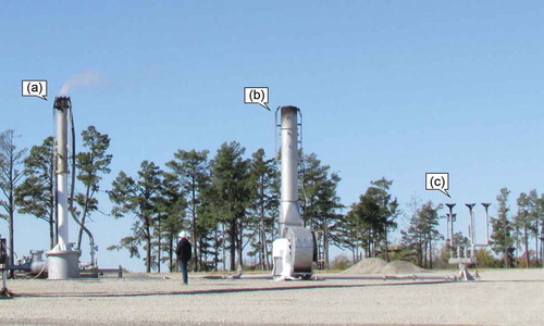
The experiment was conducted in November 2014 at the flare test facility of Zeeco, Inc., located near Tulsa, OK. Three full-scale fares were tested: a 16-inch steam assisted flare (Zeeco model QFS), a 10-inch air-assisted flare (Zeeco Model AFDS), and a multipoint sonic flare (also referred to as a pressure assisted flare and used as a ground flare; Zeeco model MPGF). is a picture of these three flares used in the experiment.
Figure 1. Three flares used in the experiment: (a) QFS steam-assisted flare; (b) AFDS air-assisted flare; and (c) MPGF multipoint sonic flare.
The experiment setup is illustrated in . For this experiment, a hyperspectral infrared (IR) imager (model SOC750 by Surface Optics Corp.) was used to image flares at a distance of 300 ft from the base of the flare stacks. The optics of SOC750 includes a 50 mm lens with a field of view (FOV) of 8.8 degrees. The SOC750 is a “staring” hyperspectral imager with 42 spectral bands in the wavelength of 2–5 µm. The spectral resolution is approximately 73 nm. As a staring imager, it has high frame rate. It is radiometrically calibrated. Its sensor is a 256 × 240 cooled midwave infrared (MWIR) focal plane array. For this experiment, the SOC750 was operated to acquire and process spectral imagery at a rate of approximately 11 data cubes (256 × 240 pixels × 42 bands) per second. For each test run, SOC750 acquired data for 30 sec, generating 325 cubes for each test run.
Figure 2. Experiment setup. (a) SOC750 hyper-spectral imager; (b) extractive sampling apparatus; and (c) gas monitoring trailer.
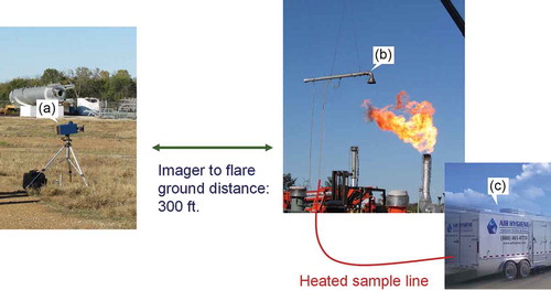
In order to validate this new method, an extractive sampling system was used (see ). An inductor with a sampling hood was suspended over the flare using a crane. A portion of the gases captured by the inductor was extracted and transported via a heated sampling line to the monitoring trailer. Inside the trailer, a contracted stack tester continuously analyzed samples for combustion products carbon dioxide (CO2) and carbon monoxide (CO), unburned hydrocarbon (HC), and oxygen (O2). The analyzers used for CO2, CO, HC, and O2 measurements were Servomex model 1440, ThermoFisher Scientific model 48C, VIG model 210, and Servomex model 1440, respectively. The test methods and procedures used were consistent with standard EPA methods for stack testing.
Thirty-nine test runs were completed (test numbers 0–39; test number 33 was aborted because the imager was not ready). The test conditions are summarized in . The flares were operated by Zeeco personnel and the information in was provided by Zeeco, except for the notes added by the authors based on observation. As discussed earlier, three types of flares were tested: air-assisted (AFDS), steam-assisted (QFS), and pressure-assisted (MPGF). Four types of fuels were used in the test: propane, propane/nitrogen blend (50:50), propylene, and natural gas. For the air-assisted flare, airflow rates are provided in with the unit of standard cubic feet per minute (SCFM). Based on the fuel flow, the amount of air supplied was also expressed as a percentage of stoichiometric air needed for the combustion. In addition to the supplied air, combustion can occur utilizing air from the atmosphere. For the steam-assisted flare, both steam rates and steam to HC ratio (on a mass basis) are provided in . also provides combustion zone net heating values (CZNHV) for air-assisted and steam-assisted flares, an important parameter used by EPA for these types of flares.
Table 1. Flare test conditions.
Among the 39 test runs, 28 were designed to validate this method using the data from the extractive sampling system. The remaining 11 of the 39 test runs were designed to test the capability of this method under some extreme conditions. Among these 11 runs, four of them (test numbers 0, 14, 15, and 16) had heavy smoke. Five of them (test numbers 10, 11, 19, 20, and 35) were operated at extremely low vent gas rates (very small flame footprints). Two of them (test numbers 12 and 13) had no vent gas and were designed to test the imager’s capability to image the pilot at the 300-ft distance.
Results and discussion
As described in the previous section, in total, 325 data cubes were acquired by the SOC750 hyperspectral imager for each of the 39 test runs. For each test run, an average data cube was derived by averaging the 325 cubes temporally. The reason for this averaging was to reduce the number of data sets to be processed manually in this study to a more manageable numbers. This averaging was appropriate because the flare was operated under a steady-state condition during each 30-sec test run and the images were inspected to ensure there was no significant change in the pattern of the flare flame. When this method is deployed in a monitoring instrument and data analysis is automated, this temporal averaging step will be eliminated to preserve the short analytical cycle in rapidly changing flare conditions. The final flare CE values can be averaged over a period of time desired by flare operators.
For each pixel of the average data cube, relative concentrations of CO2 and HC, which were represented by the IR intensities in their respective spectral bands, were used in eq (2) to calculate CE for that pixel. There were 256 × 240 pixels. For the pixels that represent the flare flame (“flame pixels”), the IR intensity was high and the CE calculation was carried out. The rest of the 256 × 240 image is background scene where the IR intensity registered by the imager was virtually zero. For these nonflame, background-scene pixels (“background pixels”), no CE values were calculated.
Within the flame pixels, there was a subset of pixels that represented an outer combustion envelope where combustion ceased. Inside the combustion envelope the combustion is still progressing, unburned hydrocarbon concentrations tended to be high (particularly at the center of the flame near the flare tip), and CE values at the pixel level tended to be low. The pixels inside the combustion envelope do not represent the CE of the flare; rather, the pixels on the outer combustion envelope represent the true CE. Therefore, only the pixels representing the outer combustion envelope were averaged to derive a single CE value, which was used to represent the flare CE during the 30-sec test run. The same approach could be used for different temporal intervals, for example, 10, 20, or 60 sec, and the resulting CE values would provide corresponding time-averaged CE for the flare being monitored.
Once the CE value was calculated using the new method, it was compared to the CE value determined by the extractive method. The extractive method generated concentrations of CO2 and HC at a 1-sec time interval. From these second-by-second CO2 and HC data, CE was calculated using eq (2) in the same way as the new method. The time stamps of both the new method and the extractive method were synchronized, and the 30-sec test period of the new method was matched with the corresponding time window in the continuous data stream generated by the extractive method. is an example showing how the two data sets are matched for test numbers 36–39. The CE values generated by the extractive method during each 30-sec data cube were averaged and compared with the CE result from the new method.
Figure 3. Example O2, CO2, and CE data from extractive method overlaid with imager test time for test numbers 36, 37, 38, and 39.
Results from 28 CE validation tests
The results of the 28 CE validation tests are summarized in . The first seven columns of data in show the flare operating data (provided by Zeeco) that were presented in and are repeated in for convenience. The “CE-extractive method” and “CE-new method” are the results from the two methods, and the column labeled “CE difference” is the difference between the two methods. The column labeled “Smoke Index” is discussed in a later section. The last column is the 30-sec average of oxygen in the extracted sample. If the value in this column is close to 21%, it suggests that the extracted sample was significantly diluted by ambient air, possibly due to positioning of the extraction hood in relation to the changing flare plume or a small flare plume. It is ideal to capture as much of the flare combustion gases as possible with minimum ambient air dilution. For this experiment, extractive sampling data points with an oxygen level less than 19.5% are considered to be a higher quality data, that is, better plume extraction and less ambient air dilution. Among the 28 tests in , 18 are in this category.
Table 2. Flare CE validation test results.
Overall, the CE values measured by the new method agree well with the CE values measured by the extractive method. The average difference between the two methods is 0.50% when all 28 tests are included. The average difference is smaller (0.10%) when only the 18 higher quality extractive data points are considered. In addition to the extractive sampling data quality, the CE level appears to play a role in the accuracy of the method. The difference between the two methods is larger when the CE is low (e.g., test numbers 32, 34, and 36, with their CE being 67.48%, 59.99%, and 70.57%, respectively). Under these low CE conditions, the new method tends to overestimate the CE when compared to the extractive results. The two methods correlate well with an r2 of 0.9856. However, the projected regression line does not pass through the origin (see ), which is consistent with the positive bias of the new method in the low CE region. It should be noted that the flares are not designed to operate with such a low CE. However, low CE conditions may occur, for example, oversteaming (Allen and Torres, Citation2011). Currently there is no practical means to alert flare operators the presence of low CE operating conditions. The new method should be capable of providing real-time CE to flare operators so that low CE (i.e., high emission) conditions can be detected and rectified.
Figure 4. Flare CE measured by extractive method and by new method in 28 validation test runs.
As the CE level in these tests increased, the hydrocarbon level decreased significantly and became particularly small in comparison to the level of CO2. For the tests that had high CE values, the hydrocarbon level was very low for both methods. In many of these tests, the hydrocarbon concentration in the extracted samples was in 0.05–1 ppm range, which was fairly close to the hydrocarbon analyzer baseline and significantly lower than the span of gas concentration of the analyzer. Similarly, the hydrocarbon peak in the imager spectral data was barely recognizable. This challenge generally exists in any instrument attempting to measure both extremely high and low concentrations at the same time. This factor could be a contributor to the difference between the two methods at high CE levels.
Duplicate test runs were conducted to provide a measure of repeatability for the new method used. Out of the 28 validation tests listed in , 26 tests were paired with a duplicate result with flare conditions held as steady as possible. Only test numbers 1 and 34 did not have a paired test. The absolute difference between the 13 paired tests was calculated separately for the extractive method and the new method. The results are summarized in . Tests 31–37 were designed to create low CE conditions by oversteaming. As a result, it was difficult to hold the flare condition constant between two duplicated tests for the desired amount of time. For two of the 13 paired tests (test numbers 31 and 32 and test numbers 36 and 37), the CE values were not repeatable. It should be noted that the difference between the extractive method and the new method in the contemporaneous time frame among these four tests actually agreed reasonably well. Excluding these two pairs that were not actually paired, the average difference in the measured CE is 0.07% and 0.20% for the extractive method and the new method, respectively. These differences suggested strong repeatability for the new method.
Table 3. Repeatability - duplicated tests.
Results for heavy smoke conditions
Flares should not be operated with visible smoke. There are regulatory limits on opacity for flare operations. Flare technology has progressed over the decades with flare manufacturers designing flares that can achieve smokeless operations by means of assisting the flare with steam, air, or pressure. One of the major findings of the 2010 TCEQ flare study is that flare CE can be severely reduced when oversteaming occurs, and the best CE is achieved when the flare is operated at an “incipient smoke point”—the condition where the steam is reduced to a point just before smoke is observed (Allen and Torres, Citation2011). In practice, it is difficult to operate a flare at an incipient point without some measure of the level of smoke in the flare plume. Relying on the operator’s visual observation of smoke is generally impractical and will be technically infeasible at night.
In addition to continuous and autonomous CE measurements, the newly proposed method can detect and measure the presence of aerosols. In the case of flare combustion, the aerosol represents soot or smoke in the flare plume. A unitless metric called the “smoke index” has been developed to measure the level of smoke, as illustrated in . An optically transparent flare plume results in a smoke index (SI) of zero, and the SI progressively increases as the smoke level in the flare plume increases. It is anticipated that flare operators can observe the flare smoke condition in conjunction with the SI provided by this new monitoring method to establish an operational SI range. When the flare is operated within this range, no visible smoke is expected. For this particular study, no visible smoke was observed when the smoke index was below 6. However, there was not a sufficient number of tests designed to cover the transition from smoke to nonsmoke conditions. Therefore, the upper limit for the operational SI range may be less than 6. Nevertheless, SI = 6 is used as a preliminary dividing line between smoke and smokeless conditions. In future tests, the flare opacity determined using EPA Method 9 can be recorded simultaneously with the SI generated by this method. If the two metrics exhibit a close correlation, the SI can be used quantitatively as a flare operational control parameter or even as a surrogate to opacity monitoring for flares.
Figure 5. Examples of smoke level and smoke index: (a) test 29, smoke index = 0.56; (b) test 18, smoke index = 2.24; (c) test 14, smoke index = 7.41; and (d) test 16, smoke index = 8.89.
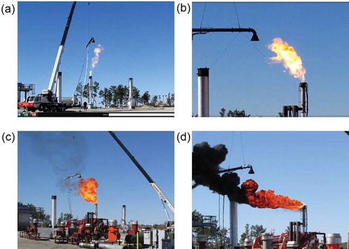
Because the new CE measurement method is an optically based method, it was expected that a significant level of smoke or soot in the flare might interfere with the CE measurement. The experiment included test conditions to study this assumption. Four tests were conducted under heavy smoke conditions and the test results are summarized in . During these four tests, air assist (test number 0) or steam assist (test numbers 14–16) was turned off, resulting in heavy smoke. In some cases, the extractive hood had to be positioned further away to avoid black smoke, as indicated by relatively high oxygen levels in the extracted samples in . The extracted samples were filtered by a sample conditioning system in the test trailer to remove soot, and the results indicated good CE values. As expected, the new method did not agree with the extractive method as well as it did under smokeless conditions in , especially for test number 15. For test number 16, the smoke was overwhelming (also see ), and the data was inadequate for CE calculation. From a practical viewpoint, bringing the flare into a smokeless condition would be a higher priority for the flare operators than getting more accurate CE readings under such a heavy smoke condition. The data from the extractive method showed that the CE was high during this heavy smoke condition.
Table 4. Flare CE tests with smoke conditions.
The significance of the SI is that it can provide a meaningful metric for flare operators to gauge the level of smoke in a flare plume from the control room day and night. The combination of the two parameters, CE and SI, in real time can provide flare operators the information needed to optimize flare operations.
Flare flame size and imager optics
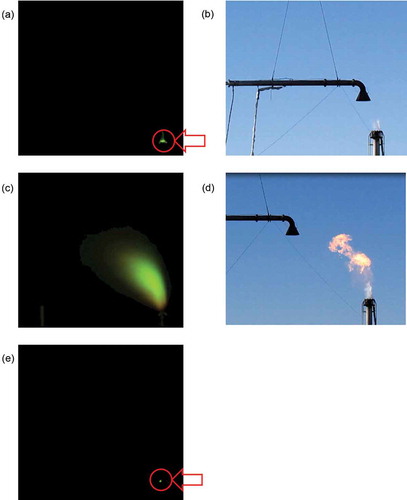
Four of the 39 test runs (test numbers 10, 11, 19, and 20) were conducted when the flare was operated at very low fuel rates (see ), This resulted in very small flame sizes in the IR images captured by the SOC750 at 300 ft ground distance. The results of these tests are summarized in , in the upper portion. To provide a perspective of the flame image sizes, both an IR image from one spectral band of SOC750 (i.e., image corresponding to one spectral slice of the 30-sec average data cube) and a snapshot visible image of test 19 (fuel rate: 237 lb/hr) are provided in , along with similar IR and visible images of test 18 (fuel rate: 4,910 lb/hr, nearly 10 times higher than test 19). The images of tests 10, 11, 19, and 20 are so small at this distance and with this lens that there are only 1–4 pixels on the outer combustion envelope (see , column labeled “Number of usable pixels”). Consequently, the CE results derived from such a small number of pixels are not very consistent with the CE results from the extractive sampling, and they are considered unreliable. Under these conditions, even the extractive sampling system may not produce reliable results because the flame is small and the hood may not capture a representative sample of combustion gases. This speculation is supported by the fact that oxygen levels in the four extracted samples were very close to the ambient air oxygen level. It should be noted that the new method made measurements based on what was in the combustion zone, whereas the extractive method was based on what was extracted. The two might not have been the same under unstable, poor combustion conditions.
Table 5. Flare CE tests at very low fuel rates and small flame sizes.
Figure 6. Images of small flare sizes and pilot: (a) IR image of Test 19; (b) visible image of test 19; (c) IR image of test 18; (d) visible image of test 18; and (e) IR image of test 13—no vent gas, lit pilot only.
Tests 34–37 were operated at high steam, low fuel conditions. The CE measured by the extractive method were low, 20.38–83.15% (see the lower portion of ). Particular attention was given to test 35, which was problematic for both methods. This test had very low CE and the flame size was so small that only 1 pixel was usable for CE calculation in the new method. It also had a near ambient air oxygen level, indicating that the extractive sampling method had poor plume extraction due to the small flame size. The discussions in the preceding paragraph are applicable to test 35. For these reasons, test 35 was excluded from validation test shown in and . The remaining three tests in this group (test numbers 34, 36, and 37) had a higher CE measured by the extractive method, better extraction indicated by oxygen levels, and most importantly more than 200 usable pixels in the SOC750 images to make CE calculations. The results of these three tests are included in and , along with other validation tests.
The issue of small flame size as it relates to the number of usable pixels in the new method (as indicated in and discussed earlier) should be viewed in the context of the distance from the imager to the flare and the optics of the imager. If a lens with a longer focal length and narrower field of view (FOV) is used, the flare image will be magnified and the number of usable pixels will increase, resulting in a suitable number of pixels for this new method. Similarly, positioning the imager closer to the flare may also yield a suitable number of usable pixels for small flame sizes. An elegant solution will be an imager equipped with two optical paths, a wider FOV when the flare is operated at high rates and a narrower FOV when the flare is operated at low rates.
Tests 12 and 13 were designed to test if the pilot of the flare could be imaged by SOC750 at this distance when there was no flame other than the small flame of the lit pilot (see ). No CE measurement was made by extractive method. However, the SOC750 was used to capture the same 30 sec of IR images as in other tests. The CE calculation was not performed because the pilot flame was too small to be represented by a sufficient number of usable pixels for the method. The image of the pilot was detected by the SOC750 (see ), which allowed for the detection of the lit pilot based on the concentration of the pilot flame combustion product (CO2). The same result was observed during test 12. Collectively, test numbers 12 and 13 suggest that the new method can be used to confirm the presence of a lit pilot, which is a critical piece of information for flare operators.
Conclusion
Operation of an industrial flare is a very dynamic process and the combustion efficiency (CE) of the flare is of utmost importance. Currently there is no method to directly measure flare CE in real time and to provide feedback for control and optimization of such a dynamic process. The experiment conducted on three of the most common types of flares (steam-assisted, air-assisted, and pressure-assisted flares) has demonstrated the technical feasibility of using a hyperspectral or multispectral staring infrared imager to directly and remotely measure flare CE. Thirty-nine tests were conducted using this new method and a conventional extractive method simultaneously to evaluate the capability and validity of the new method. While the extractive method is not practical for routine operations due to the cumbersome and manual extraction process, it does serve the purpose of providing validation for the new method. The 28 validation tests have shown strong agreement between the two methods with an average difference of 0.50% in CE measurement, and strong correlation with an r2 of 0.9856. In 11 pairs of duplicated tests conducted under steady flare operating conditions, the average absolute difference between duplicated tests is 0.20% while the same measurement is 0.07% for the extractive method, indicating good repeatability for both methods.
The new method utilizes an imager to collect data. The entire flare is imaged and the data from the outer combustion envelope are used to determine the combustion efficiency. Unlike path-based optical measurement techniques, the imaging capability of this new method eliminates the need for aiming the optical path at certain regions of the flare plume where the combustion has completed and it can tolerate variability of the flare influenced by atmospheric conditions.
The new method also provides a metric called the smoke index, which serves as an indicator for level of smoke in the flare plume. The smoke index is a unitless metric derived from the IR characteristics of soot in the flare plume, and it should monotonically vary with the level of smoke. In a future study, it will be worthwhile to explore the relationship between the smoke index and the opacity of the flare.
Recent studies have concluded that performance is the best when the flare is operated near the incipient smoke point. To achieve this optimal operating condition, flare operators need to strike a balance between CE and the level of smoke, and both these parameters are currently not available to operators. The new method will provide both metrics continuously and in real time.
The new method can be applied to various sizes of flares. Although the method needs a reasonable number of pixels representing the flare plume, this requirement can be met by combination of imager’s optics (i.e., field of view or magnification power) and the distance between the flare and the imager.
Acknowledgments
The authors thank Zeeco, Inc., for providing its flare test facility for this study. Specifically, the support provided by Scot Smith, Doug Allen, Kristen Weidner, Garrett Midgley, Cody Little, and others at Zeeco was greatly appreciated.
Funding
This work was partially funded by the EPA through its Small Business Innovative Research (SBIR) program under contract EP-D-15-012.
Additional information
Funding
Notes on contributors
Yousheng Zeng
Yousheng Zeng, Ph.D., and Jon Morris, M.S., are chief executive officer (CEO) and chief technical officer (CTO), respectively, of Providence Photonics, based in Baton Rouge, LA.
Mark Dombrowski
Mark Dombrowski, B.S., is Vice-President of Surface Optics Corp., based in San Diego, CA.
References
- Allen, D.T., and V.M. Torres. 2011. TCEQ 2010 flare study final report. Prepared for TCEQ. PGA No. 582-8-862-45-FY09-04 with supplemental support from TCEQ grant 582-10-94300. http://www.tceq.texas.gov/assets/public/implementation/air/rules/Flare/2010flarestudy/2010-flare-study-final-report.pdf (accessed March 23, 2015).
- ENVIRON. 2008. Cost analysis of HRVOC controls on polymer plants and flares. Report prepared for Texas Commission on Environmental Quality, Project 2008-104, Work Order 582-07-84005-FY08-12. http://www.tceq.state.tx.us/assets/public/implementation/air/rules/Flare/HRVOC_Cost_Analysis_Report.pdf (accessed March 23, 2015).
- Farina, M.F. 2011. Flare gas reduction—Recent global trend and policy considerations. GE Energy Global Strategy and Planning, GEA18592 (10/2010). http://www.genewscenter.com/ImageLibrary/DownloadMedia.ashx?MediaDetailsID=3691 (accessed January 17, 2014).
- U.S. Environmental Protection Agency. 2012. Parameters for properly designed and operated flares. EPA Office of Air Quality Planning and Standards (OAQPS). http://www.epa.gov/ttn/atw/flare/2012flaretechreport.pdf (accessed March 24, 2015).
- U.S. Environmental Protection Agency. 2014. Fact sheet, Proposed petroleum refinery sector risk and technology review and new source performance standards. http://www.epa.gov/airtoxics/petrefine/20140515factsheet.pdf (accessed on March 24, 2015).
- Zeng, Y., J. Morris, and M. Dombrowski. 2012. Multi-spectral infrared imaging system for flare combustion efficiency monitoring. Provisional patent application 61/662,781 filed with the U.S. Patent and Trademark Office on June 21, 2012 and utility patent application S.N. 13/850,832 filed on March 26, 2013.