Collocated comparisons of continuous and filter-based PM_2.5 measurements at Fort McMurray, Alberta, Canada

ABSTRACT

Collocated comparisons for three PM_2.5 monitors were conducted from June 2011 to May 2013 at an air monitoring station in the residential area of Fort McMurray, Alberta, Canada, a city located in the Athabasca Oil Sands Region. Extremely cold winters (down to approximately −40°C) coupled with low PM_2.5 concentrations present a challenge for continuous measurements. Both the tapered element oscillating microbalance (TEOM), operated at 40°C (i.e., TEOM₄₀), and Synchronized Hybrid Ambient Real-time Particulate (SHARP, a Federal Equivalent Method [FEM]), were compared with a Partisol PM_2.5 U.S. Federal Reference Method (FRM) sampler. While hourly TEOM₄₀ PM_2.5 were consistently ~20–50% lower than that of SHARP, no statistically significant differences were found between the 24-hr averages for FRM and SHARP. Orthogonal regression (OR) equations derived from FRM and TEOM₄₀ were used to adjust the TEOM₄₀ (i.e., TEOM_adj) and improve its agreement with FRM, particularly for the cold season. The 12-year-long hourly TEOM_adj measurements from 1999 to 2011 based on the OR equations between SHARP and TEOM₄₀ were derived from the 2-year (2011–2013) collocated measurements. The trend analysis combining both TEOM_adj and SHARP measurements showed a statistically significant decrease in PM_2.5 concentrations with a seasonal slope of −0.15 μg m⁻³ yr⁻¹ from 1999 to 2014.Implications: Consistency in PM_2.5 measurements are needed for trend analysis. Collocated comparison among the three PM_2.5 monitors demonstrated the difference between FRM and TEOM, as well as between SHARP and TEOM. The orthogonal regressions equations can be applied to correct historical TEOM data to examine long-term trends within the network.

Introduction

Epidemiological studies have found associations between particulate matter (PM) concentrations and adverse health effects (Chow et al., 2006a; Pope and Dockery, 2006; USEPA, 2004; Vedal, 1997; Watson et al., 1997). In 2013, PM from outdoor air pollution was classified as carcinogenic to humans by the International Agency for Research on Cancer (Loomis et al., 2013). PM also causes visibility impairment (Chow et al., 2002; Watson, 2002) and affects the earth’s thermal radiation balance (Fiore et al., 2015).

PM_2.5 and PM₁₀ (particulate matter with aerodynamic diameters less than 2.5 and 10 µm, respectively) concentrations are indicators of adverse health effects (Bachmann, 2007). Canadian Ambient Air Quality Standards (CAAQS) for PM_2.5 replaced the Canada-Wide Standard (CWS), reducing 24-hr PM_2.5 levels from 30 to 28 μg m⁻³ with an annual average of 10 µg m⁻³ (https://www.ec.gc.ca).

CAAQS and CWS compliance is determined by measurements made with Federal Reference Methods (FRMs) or Federal Equivalent Methods (FEMs) developed by the U.S. Environmental Protection Agency (U.S. EPA) (USEPA, 2014). The tapered element oscillating microbalance (TEOM) monitor (model 1400a, Rupprecht & Patashnick, now Thermo Scientific, Waltham, MA) has been designated as a PM₁₀ FEM since 1990 (USEPA, 2014). The TEOM PM₁₀ monitor, configured with either a sharp cut cyclone (SCC) or a very sharp cut cyclone (VSCC, BGI, now Mesa Labs, Inc., Lakewood, CO) (Watson and Chow, 2011), monitored PM_2.5 (Sofowote et al., 2014) before designation of FEMs PM_2.5.

To determine compliance with CAAQS, PM_2.5 measurements have been acquired as part of the Wood Buffalo Environmental Association (WBEA, www.wbea.org) air quality monitoring network in northeastern Alberta, Canada, where TEOM monitors (model 1400a) with SCC (or VSCC) inlets measured hourly PM_2.5 from 1999 to 2011. These instruments operated at 40°C, as specified by Alberta Environment and Sustainable Resource Development. After June 2009, Synchronized Hybrid Ambient Real-time Particulate (SHARP) monitors (model 5030, Thermo Scientific, Waltham, MA), designated as Class III PM_2.5 FEMs by the U.S. EPA (2009), were installed as replacements for the aging TEOMs. PM_2.5 from collocated TEOM and SHARP monitors show differences that affect the interpretation of long-term trends (Ayers et al., 1999; Bencs et al., 2010; Charron et al., 2004; Chow et al., 2008; Chow et al., 2006b; Cyrys et al., 2001; Hauck et al., 2004; Sofowote et al., 2014; Zhu et al., 2007). The extremely low temperatures (e.g., –40°C) and low PM_2.5 concentrations (e.g., annual average of ~5 µg m⁻³) in the Athabasca Oil Sands Region (AOSR, northeastern Alberta, Canada) present further challenges for consistent PM_2.5 measurements. The objectives of this study were to (1) evaluate the similarities and differences of PM_2.5 mass concentrations measured by collocated FRM samplers (Partisol, Thermo Scientific) and continuous TEOM and SHARP monitors; (2) examine relationships among the three measurements that might allow one to be predicted from another; and (3) determine the extent to which the TEOM PM_2.5 measurements can be adjusted to understand PM_2.5 trends since 1999.

Methodology

Site description

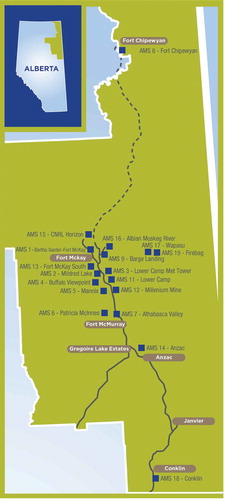
PM_2.5 was measured at four neighborhood-scale air monitoring stations (AMS) that are part of the WBEA monitoring network, shown in Figure 1. These include: (1) AMS 1 (57.189 N, 111.640 W) in a nonurban community ~58 km north-northwest of Fort McMurray in the First Nation and Métis Community of Fort McKay; (2) AMS 6 (56.751 N, 111.476 W) in an urban/residential area of Fort McMurray; (3) AMS 7 (Athabasca River valley in downtown, 56.732 N, 111.390 W) in the populated city of Fort McMurray (~61,300 residents); and (4) AMS 14 (~35 km southeast of Fort McMurray, 56.449 N, 111.037 W) in the nonurban residential area of Anzac. Both Fort McKay and Anzac contain only 550–600 inhabitants (www.statcan.gc.ca). Fort McKay is surrounded by AOSR mining activities. PM_2.5 concentrations in this region are affected by emissions from engine exhaust, cooking, residential wood combustion, and forest fires, as well as resuspended dust from paved/unpaved roads, construction, and mining activities (Wang et al., 2015a, 2015b, 2016; Watson et al., 2014; Watson et al., 2012).

Figure 1. WBEA ambient air quality monitoring stations in the Athabasca Oil Sands Region (AOSR) in northern Alberta Canada (www.wbea.org). PM_2.5 was measured at the nonurban communities of Fort McKay (AMS 1) and Anzac (AMS 14), as well as at the urban area of Fort McMurray (AMS 6 and 7).

PM_2.5 measurements

Tapered element oscillating microbalance (TEOM)

The TEOM collects PM on a vibrating substrate and measures the change in the oscillation frequency (Patashnick and Rupprecht, 1991) that decreases with mass loading. Operation of TEOM requires a constant temperature setting above ambient (typically 30–50°C) to prevent expansion and contraction of the tapered element and reduce interference from water vapor condensation. However, heating the ambient air enhances volatilization of particle-bound semivolatile compounds (e.g., ammonium nitrate and some organic species) (Ayers et al., 1999; Charron et al., 2004). This volatilization results in an underestimation of PM_2.5 mass, especially when semivolatile compounds favor the particulate phase during cold seasons (Allen et al., 1997; Rees et al., 2004).

Synchronized Hybrid Ambient Real-time Particulate (SHARP)

The SHARP monitor measures the photometric signal by light scattering in the sampling duct and the attenuation of an electron beam (beta rays) transmitted through particles collected on a filter tape. Both can be related to PM_2.5 mass, assuming certain particle sizes, shapes, and compositions. The relationship between monochromatic light scattered by an ensemble of particle sizes and numbers is (Gebhart, 2001; Thomas and Gebhart, 1994)

(1)

where P is scattered light flux collected by the detector, I₀ is the incident flux, V_m is the sensing volume, C_n is the total particle number concentration, f(d_p) is the particle number-based size distribution, d_p is particle diameter, S is the power of light scattered by a particle over the light-collecting solid angle of the scattered light detector, λ is wavelength, and m is refractive index. Light scattering can be measured with high time resolution (~1 sec). For particles with the same size distribution and composition, scattered light is proportional to the number or mass concentration (Wang et al., 2009). However, photometric measurements underestimate ultrafine (d_p < 0.1 µm) and large (> 2.5 μm) particle contributions when calibrated with aerosols typical of PM_2.5. Relationships between scattered light and particle concentration vary by location and season (Chow et al., 2006b). To account for the variable relationships between mass and particle light scattering, the SHARP periodically (every few hours) normalizes the scattering to the beta attenuation mass.

Beta attenuation is related to mass concentration by (Jaklevic et al., 1981)

(2)

where β is the transmitted electron flux, β₀ is the incident electron flux, µ is the mass absorption coefficient (cm² g⁻¹), and x is the mass thickness of the sample (g cm⁻²) (Kulkarni et al., 2011); μ is determined by comparing standards of known mass to β.

The light scattering-derived PM_2.5 mass concentration is

(3)

where N_ave is the 1-min average concentration (µg m⁻³) derived from light scattering, and B/N, a correction factor, is the ratio of concentrations between beta attenuation (B) and light scattering (N). A time constant, a function of the coefficient of variation of the light scattering signal, ranging from 20 to 480 min, is required to obtain the B/N ratio. To reduce the interference from water vapor, SHARP is equipped with a heating system that turns on when the relative humidity (RH) exceeds 35%. Because of the lower saturation water vapor pressure on cold days, only mild heating is needed. For example, heating the sampled air stream from –40°C to –9°C reduces the RH from 100% to 34%. Less heat is required to maintain RH at <35% in SHARP than for the TEOM samples at 40°C (i.e., TEOM₄₀). This results in lower losses of semivolatile compounds in the SHARP than in the TEOM.

Collocated comparisons were conducted over a period of 2 years (June 2011 to May 2013) for Partisol FRM, TEOM₄₀, and SHARP (all from Thermo Scientific) at the AMS 6 (residential Fort McMurray) site to determine how well one method compares with the others. Collocated FRM and TEOM₄₀ measurements were also acquired at the other three sites (i.e., AMS 1, 7, and 14) from February to August 2011 to evaluate the generality of the derived relationships. Both TEOM₄₀ and SHARP monitors were operated in temperature-controlled (22−25°C) shelters, while the Partisol FRM was on the shelter rooftop. Each of the three monitors was equipped with a VSCC size-selective inlet (~3 m above ground level). Twenty-four-hour Teflon-membrane filter samples (midnight to midnight) were collected every 6 days following the Canadian National Air Pollution Surveillance (NAPS) schedule. In addition to daily flow and display checks, routine maintenance (e.g., inlet cleaning and leak checks) was carried out on a monthly basis, and that frequency was increased when necessary. Greater detail is found in the standard operating procedures (http://www.wbea.org/air-monitoring/standard-operating-procedures).

Teflon-membrane filters for the FRM were equilibrated in a temperature (20–30°C) and RH (30–40%) controlled environment for >48 hr before the pre- and postsampling gravimetric analyses on a microbalance with ±1 μg sensitivity. Hourly PM_2.5 raw data from the TEOM₄₀ and SHARP monitors were retrieved from the data logger and archived in WBEA’s database. These Level 1 (L1) data were then reviewed monthly as part of the quality control (QC) and quality assurance (QA). Following the Air Monitoring Directive specified by the government of Alberta, negative TEOM values (often found during the cold seasons) were replaced by zeros for concentrations ranging from –3.0 to 0.0 μg m⁻³ and should be invalidated for concentrations <–3.0 μg m⁻³ as part of the Level 2 (L2) validation criteria (Alberta Environment and Sustainable Resource Development [AESRD], 2014). With an internal heating system, negative values were seldom found with the SHARP monitor. Although a common practice in cold environments caused by slowly evaporating compounds coupled with low PM concentrations, this zero adjustment approach yields a small positive bias to PM_2.5 concentrations (e.g., 24-hr, monthly, and annual averages), but it does not compensate for the TEOM₄₀’s negative bias. Both L1 and L2 data are available at http://www.wbea.org/monitoring-stations-and-data/historical-monitoring-data.

Statistical analysis

Nonparametric statistical analyses were employed (Hsu, 2013), including (1) Mann–Whitney rank sum test (Sigmaplot 11, San Jose, CA); (2) Spearman rank order correlation (SigmaPlot 11); (3) Mann–Kendall trend analysis (XLSTAT-Time, Addinsoft, New York, NY); and (4) Sen trend analysis (XLSTAT-Time). In addition, two regression analyses were applied: (1) simple linear regression analysis (SLR, Excel 2013, Redmond, WA) to assess the association between the independent and dependent variables without consideration of measurement uncertainties; and (2) orthogonal regression (OR; Minitab 16, State College, PA), which recognizes measurement uncertainties in both variables (Hauck et al., 2004). Pearson correlation coefficients (Excel 2013, Redmond, WA) and Spearman rank order correlation coefficients were calculated for the SLR and OR analyses, respectively.

Results and discussion

Hourly PM_2.5 concentrations from TEOM₄₀ and SHARP

The average and median for TEOM₄₀ PM_2.5 at the AMS 6 site from June 2011 to May 2013 were 4.3 and 2.3 µg m⁻³ (with 25th and 75th percentiles of 0.72 and 4.9 µg m⁻³, respectively). During the cold season (from November to April), snow cover minimizes fugitive dust emissions, although resuspension of deicing materials counters this reduction during thawing. Low temperatures cause more semivolatile species to condense, resulting in higher PM_2.5 mass with increased particle-phase ammonium (NH₄⁺), nitrate (NO₃⁻), and organic carbon (OC) (Chen et al., 2012; Green et al., 2015; Hsu and Clair, 2015). Major PM sources during the warm season (from May to October) are fugitive dust from paved and unpaved roads, construction, and mining activities, based on the 2009 National Pollutant Release Inventory published by Environment Canada (2011).

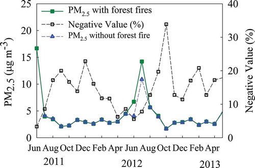
Figure 2 shows that monthly-average TEOM₄₀ PM_2.5 varied from 1.7 to 17 µg m⁻³. The two elevated monthly PM_2.5 concentrations (i.e., June 2011 and July 2012) corresponded with forest fires in the region, a common occurrence during summertime. PM_2.5 concentrations exceeded the maximum operation range of 450 µg m⁻³ for TEOM₄₀ with forest fires during May/June 2011. The percentage of negative hourly TEOM₄₀ PM_2.5 concentrations was more pronounced in winter than in summer. Approximately one-third (34%) of TEOM₄₀ PM_2.5 concentrations were negative during October 2012, coinciding with the lowest monthly average of 1.7 μg m⁻³.

Figure 2. Monthly average TEOM₄₀ PM_2.5 concentrations (µg m⁻³) with and without forest fires and percentage of hourly concentrations with all negative values for the residential Fort McMurray site (AMS 6) from June 2011 to May 2013. The data completeness criteria are: (1) the daily 24-hr PM_2.5 concentration is only valid if at least 75% (18 hr) of the 1-hr concentrations are available on the given day; and (2) there are at least 75% valid daily 24-hr PM_2.5 concentrations in the month.

Collocated comparison in Figure 3 shows higher PM_2.5 for SHARP compared to TEOM₄₀, with the exception of July 2012. Differences were largest when PM_2.5 was either high (e.g., 84 µg m⁻³ in June 2011) or low (e.g., 22 µg m⁻³ in January 2013) and can be attributed to the enhanced volatilization and frequent occurrence of negative concentrations for TEOM₄₀.

Figure 3. Collocated PM_2.5 TEOM₄₀ and SHARP concentrations with median, 5th, 10th, 25th, 75th, 90th, and 95th percentiles at the AMS 6 site from June 2011 to May 2013. (Note: The 95th percentile PM_2.5 concentrations in June 2011 were 71 and 90 µg m⁻³ for TEOM₄₀ and SHARP measurements, respectively.)

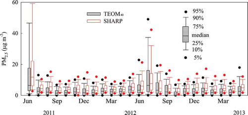
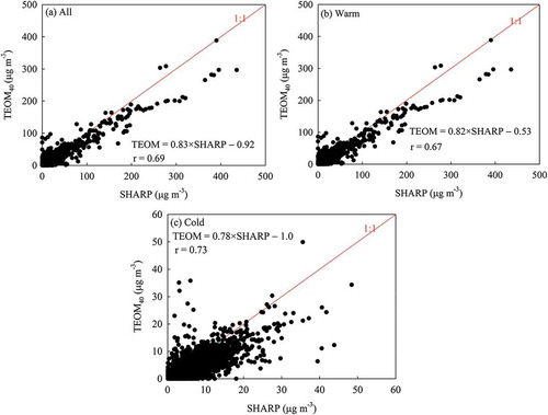
Similar OR slopes (0.82 and 0.78) were found for the warm and cold seasons (Figure 4), with consistent 20–30% lower PM_2.5 by TEOM₄₀. The largest discrepancy is found for PM_2.5 > 20 μg m⁻³. The correlation coefficients are higher for the cold (r = 0.73) than for the warm (r = 0.67) seasons. Table 1 shows nearly a factor of 2 difference (p < 0.01) in median PM_2.5 concentrations, ranging from 2.1 to 2.6 µg m⁻³ for TEOM₄₀ and from 4.1 to 4.6 µg m⁻³ for SHARP.

Table 1. Mann–Whitney rank sum tests for the 25th, 50th, and 75th percentile of hourly PM_2.5 concentrations (µg m⁻³) from the collocated TEOM₄₀ and SHARP measurements at the residential Fort McMurray (AMS 6) site from June 2011 to May 2013.

Season	Group	N (size)	25th Percentile	50th Percentile	75th Percentile	Mean	p Value
Warm	SHARP^a	7950	2.6	4.6	7.9	7.7	<0.001
	SHARP^b,c	7937	2.6	4.6	8.0	7.7
	TEOM40^a	7950	0.68	2.5	5.8	5.6
	TEOM40^b	7937	0.68	2.5	5.8	5.6
	TEOM40^c	7937	0.77	2.6	5.9	5.8
Cold	SHARP^a	8591	2.5	4.1	6.3	5.0	<0.001
	SHARP^b,c	8574	2.5	4.1	6.3	5.0
	TEOM40^a	8591	0.67	2.1	4.2	2.8
	TEOM40^b	8574	0.69	2.1	4.2	2.8
	TEOM40^c	8574	0.70	2.1	4.2	2.9
All	SHARP^a	16541	2.5	4.3	7.0	6.3	<0.001
	SHARP ^b	16511	2.5	4.3	7.0	6.3
	TEOM40^a	16541	0.68	2.3	4.8	4.1
	TEOM40^b	16511	0.69	2.3	4.8	4.1
	TEOM40^c	16511	0.73	2.3	4.9	4.3

Notes. 25^th, 50^th, and 75^th percentiles were computed from all the observations. SHARP^a: All SHARP data. SHARP^b,c: SHARP data excluding periods when TEOM data <-3.0 µg m⁻³. TEOM₄₀^a: All TEOM data (Level 1A, including all negative data). TEOM₄₀^b: TEOM data excluding <–3.0 µg m⁻³ but including those –3.0 to 0.0 µg m⁻³. (Level 1B). TEOM₄₀^c: TEOM data excluding <–3.0 µg m⁻³ and replacing those –3.0 to 0.0 µg m⁻³ with 0.0 µg m⁻³ (Level 2).

Figure 4. Two-year collocated comparison (June 2011 to May 2013) of hourly PM_2.5 concentrations by TEOM₄₀ and SHARP at the AMS 6 site for (a) entire sampling period, (b) warm season (May to October), and (c) cold season (November to April).

During the 2-year collocated comparison, negative (>–3.0 µg m⁻³) PM_2.5 concentrations were found for 14% (n = 2452) of TEOM₄₀ hourly averages. As shown in Table 2, similar averages (–0.81 µg m⁻³ for n = 2482 and –0.77 µg m⁻³ for n = 2452) were found between Level 1A (TEOM₄₀ was smaller than 0.0 µg m⁻³) and Level 1B (TEOM₄₀ was between –3.0 and 0.0 µg m⁻³), with the 50th percentile of –0.62 to –0.63 µg m⁻³. This is expected, as only ~1% of the hourly measurements were below –3 µg m⁻³. Assuming the SHARP PM_2.5 concentration is correct (no negative values found) for TEOM PM_2.5 concentration smaller than 0.0 µg m⁻³, replacing negative values with zero in the database (i.e., Level 2) resulted in an underestimate of approximately –2.0 µg m⁻³ (50th percentile or median) in TEOM₄₀, which is consistent with those shown in Table 1.

Table 2. Comparison between TEOM₄₀ PM_2.5 (<0.0 µg m⁻³) and corresponding SHARP concentrations using different validation criteria.

	TEOM40^a	SHARP^a	TEOM40^b	TEOM40^c	SHARP^b,c
Averacge ± SD (μg m^−3)	–0.81±0.73	2.7±1.7	–0.77±0.61	0±0	2.7±2.1
Number	2482	2482	2452	2452	2452
25th Percentile (μg m^−3)	–1.2	1.6	–1.1	0	1.6
50th Percentile (μg m^−3)	–0.63	2.1	–0.62	0	2.1
75th Percentile (μg m^−3)	–0.29	3.3	–0.29	0	3.3

Note. See definitions of TEOM₄₀ and SHARP in Table 1 footnote.

Comparison of 24-hr PM_2.5 concentrations among FRM, TEOM₄₀, and SHARP

Since PM_2.5 concentrations, compositions, and physical properties (e.g., refractive index, density, and size distribution) change during forest fires, a comparison was made between periods with and without forest fires. Scatter plots in Figure 5 show that the highest correlations (0.93 < r < 0.96) between the FRM and continuous monitors (i.e., SHARP and TEOM₄₀) were found during forest fires, along with higher intercepts (2.6−3.1 μg m⁻³). The higher intercepts may result from a positive organic artifact (Chow et al., 2010; Watson et al., 2009) due to the abundant volatile organic compounds (VOCs) emissions during forest fires. Future studies should include collocated FRMs with quartz-fiber backup filters for representative blank subtraction. With zero intercept, the slope increased from 0.74 to 0.79 for FRM versus SHARP and from 0.92 to 0.97 for FRM versus TEOM₄₀. Higher PM_2.5 mass in SHARP than FRM during forest fires is attributed to enhanced particle scattering, especially during the smoldering phase of combustion. Past studies (Hsu and Clair, 2015; Spracklen et al., 2007) have shown increases in NH₄⁺, NO₃⁻, OC, and elemental carbon (EC) concentrations during forest fires. The FRM PM_2.5 might not properly collect the semivolatile material due to the volatilization losses from the Teflon-membrane filter (Ashbaugh and Eldred, 2004; Chow et al., 2005; Long et al., 2003).

Figure 5. Collocated comparison (June 2011 to May 2013) between 24-hr PM_2.5 concentrations by FRM (Partisol) and continuous monitors (SHARP and TEOM₄₀) at the AMS 6 site using orthogonal regression for (a) non-forest-fire period (note different scales); (b) forest-fire period; and (c) entire sampling period. Warm (May to October) and cold (November to April) season comparisons are also shown for non-forest-fire periods in Figure 5a.

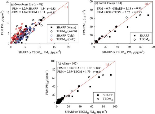
The median 24-hr PM_2.5 concentrations in Table 3 range from 3.6 to 4.5 µg m⁻³ for the FRM, but they are consistent at 4.3 µg m⁻³ for the SHARP and from 2.4 to 2.5 µg m⁻³ for the TEOM₄₀, irrespective of season. Mann–Whitney rank sum tests yield no statistically significant differences between the FRM and SHARP for any season, with p values ranging from 0.33 to 0.82. However, TEOM₄₀ PM_2.5 medians were statistically significantly lower (p < 0.01) than those of FRM and SHARP for all seasons except the warm season for TEOM₄₀ and FRM (p = 0.08).

Table 3. Mann–Whitney rank sum tests for the 25th, 50th, and 75th percentiles of 24-hr average PM_2.5 concentration (µg m⁻³) for the collocated Partisol FRM, SHARP, and TEOM₄₀ measurements at the AMS 6 site for the period of June 2011 to May 2013.

Season	Group	N (size)	25%	50%	75%
Warm	FRM	31	2.3	3.6	6.7
	SHARP	31	3.3	4.3	5.6
	TEOM40	31	1.3	2.5	4.6
	p = 0.33 between SHARP and FRM; p = 0.08 between TEOM40 and FRM; p < 0.01 between SHARP and TEOM40.
Cold	FRM	56	2.9	4.5	6.2
	SHARP	56	3.5	4.3	6.1
	TEOM40	56	1.5	2.4	3.7
	p = 0.82 between SHARP and FRM; p < 0.01 between TEOM40 and FRM; p < 0.01 between SHARP and TEOM40.
All	FRM	87	2.7	4.4	6.2
	SHARP	87	3.3	4.3	5.8
	TEOM40	87	1.5	2.4	3.8
	p = 0.44 between SHARP and FRM; p < 0.01 between TEOM40 and FRM; p < 0.01 between SHARP and TEOM40.

Although the OR slopes of FRM versus SHARP (1.25) and FRM versus TEOM₄₀ (1.16) for the non-forest-fire periods exceed unity, comparable PM_2.5 concentrations are found between FRM and SHARP during cold seasons (blue squares in Figure 5a). Forcing the intercept to zero, Table 4 shows that the ratios of FRM to SHARP are 0.99 for cold seasons and 0.97 for warm seasons, based on SLR. SHARP PM_2.5 are lower than FRM during the warm seasons and when PM_2.5 < ~6 μg m⁻³. Figure 5a shows that FRM PM_2.5 are systematically higher than TEOM₄₀ in both cold and warm seasons. For the entire sampling period, Figure 5c shows reasonable correlations (r = 0.83–0.84) between the FRM and continuous monitors, with slopes ranging from 0.78 to 0.95.

Table 4. Summary statistics of regression analysis between the collocated PM_2.5 measurements at the AMS 6 site for the non-forest-fire period of June 2011 to May 2013, with data from Environment Canada included for comparison.

Method comparison (Y/X)	Season^a	Slope (Y/X)	Intercept (μg m^−3)	r^b	Reference
FRM/SHARP	Cold (2013)	1.05	0.35	–	Environment Canada (http://www.ec.gc.ca/) (simple linear regression, SLR)
FRM/SHARP	Warm (2013)	0.99	0.22	–
FRM/TEOM40	Cold (2012)	1.3	0.94	–
FRM/TEOM40	Warm (2012)	0.94	1.72	–
FRM/TEOM40	Cold	0.88	2.20	0.71	This study (simple linear regression, SLR)
FRM/TEOM40	Warm	0.97	1.19	0.91
FRM/SHARP	Cold	1.02	–0.19	0.83
FRM/SHARP	Warm	1.10	–0.81	0.91
FRM/TEOM40	Cold	1.45	Intercept = 0	0.45
FRM/TEOM40	Warm	1.17		0.88
FRM/SHARP	Cold	0.99		0.83
FRM/SHARP	Warm	0.97		0.91
SHARP/TEOM40	Cold	1.28	1.27	0.73	This study (orthogonal regression, OR)
SHARP/TEOM40	Warm	1.21	0.64	0.67
SHARP/TEOM40	All	1.22	0.87	0.69
FRM/TEOM40	Cold	1.36	0.87	0.78
FRM/TEOM40	Warm	1.08	0.82	0.79
FRM/TEOM40	All	1.16	1.11	0.81
FRM/SHARP	Cold	1.27	–1.38	0.84
FRM/SHARP	Warm	1.23	–1.42	0.77
FRM/SHARP	All	1.25	–1.34	0.83

Notes. ^aCold and warm seasons are November to April and May to October, respectively.

^bParson correlation coefficient and Spearman rank order correlation coefficient were calculated for SLR and OR, respectively.

For non-forest-fire periods, Table 4 shows that the largest intercept, 2.2 μg m⁻³ with a slope of 0.88, was found by SLR for FRM versus TEOM₄₀ PM_2.5 during cold seasons. This differs from the OR result, which shows a lower intercept (0.87 μg m⁻³) and a higher slope (1.36). Setting the intercept to zero results in an FRM versus TEOM₄₀ slope of 1.45 and 1.17 for the cold and warm seasons, respectively, which is consistent with 20–50% losses of volatilized PM_2.5 with TEOM₄₀. FRM and SHARP comparisons are better, with ratios of 0.97–0.99 using zero intercept. Table 4 shows that the SLR regression equations developed in this study are similar to those found for other sites in Canada with TEOM₄₀ (http://www.ec.gc.ca), in that: (1) the slopes of FRM versus TEOM₄₀ are close to 1, within ~ ±30%; and (2) the slopes of FRM versus SHARP are closer to 1, within ~±10%.

Application of regression statistics to long-term databases

By incorporating measurement uncertainties, OR is a better metric than SLR for evaluating whether or not two tested variables (Y vs. X) are equivalent. The OR relationships between FRM and TEOM₄₀ measurements at the AMS 6 site were used to adjust TEOM₄₀ PM_2.5 at the other sites (i.e., TEOM_adj):

(4)

(5)

(6)

(7)

(8)

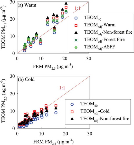
These relationships were applied to 44 sets of data from 2011 to evaluate their applicability at AMS 1, AMS 7, and AMS 14. During May to August, TEOM_adj was closer to the 1:1 line for PM_2.5 < 10 μg m⁻³, but it overestimated the FRM for PM_2.5 > 10 µg m⁻³ (Figure 6a). However, the number of data points (n = 15) for PM_2.5 > 10 μg m⁻³ was small.

Figure 6. Comparison of TEOM₄₀ and TEOM_adj (corrected with developed OR equations) with FRM PM_2.5 concentrations for (1) warm (May to August), and (2) cold (February to April) months of 2011. (TEOM_adj, Level 2 data replacing –3.0 to 0 μg m⁻³ with zero and invalidating data <–3.0 μg m⁻³; Non-forest fire, days excluding forest fires; Forest Fire, days with forest fires; ASFF, all seasons with forest fire.)

The relative differences (D, %) is

(9)

where TEOM represents either TEOM₄₀ (no correction) or TEOM_adj (using eqs 4 and 5). While D ranges from 13 to 15% for PM_2.5 < 10 µg m⁻³, these differences decrease to ~9% for PM_2.5 > 10 µg m⁻³ with TEOM₄₀ or TEOM_adj for all seasons with forest fires (ASFF). Comparability between FRM and TEOM_adj improves for the non-forest-fire period (February to April, n = 29). As shown in Figure 6b, the difference decreases from 18% for TEOM₄₀ to 13% for TEOM_adj.

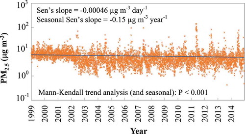
The OR equations (eqs 10–12) between SHARP (i.e., FEM) and TEOM₄₀ were applied to historical hourly TEOM₄₀ PM_2.5 concentrations at the AMS 6 site from January 1999 to August 2012 for trend analysis:

(10)

(11)

(12)

Table 5 demonstrates data completeness (91−100%) within Alberta Air Monitoring Directive specifications (AESRD, 2014), with the exception of 2005 (87%). Maximum hourly PM_2.5 varied by more than sevenfold, ranging from 73 μg m⁻³ in 2005 to 549 μg m⁻³ in 2011 (due to forest fires). The median concentrations varied more than twofold, ranging from 3.3 μg m⁻³ in 2005 to 7.7 μg m⁻³ in both 1999 and 2001. Annual averages ranged from 4.8 μg m⁻³ in 2005 to 9.3 μg m⁻³ in 2011 (and 9.1 μg m⁻³ in both 1999 and 2001), lower than the current CAAQS of 10 µg m⁻³ for PM_2.5.

Table 5. Descriptive statistics of TEOM_adj^a PM_2.5 (from January 1999 to August 2011) and SHARP PM_2.5 (from September 2011 to December 2014) concentrations (μg m⁻³) for the AMS 6 site.

Statistic	1999	2000	2001	2002	2003	2004	2005	2006	2007	2008	2009	2010	2011	2012	2013	2014
Number of observations	8760	8784	8760	8760	8760	8784	8760	8760	8760	8784	8760	8760	8760	8784	8760	8760
Completeness (%)	91	100	99	97	98	96	87	95	97	97	93	92	94	98	98	98
Maximum	221	182	124	335	78	106	73	275	303	220	340	92	549	377	140	218
25th Percentile	5.6	5.3	5.6	2.6	1.8	2.1	1.7	2.1	2.0	2.2	2.1	2.3	2.1	2.2	2.7	2.4
Median	7.7	7.3	7.7	4.8	3.6	4.3	3.3	4.0	3.7	4.4	3.9	4.3	4.0	4.2	4.3	4.3
75th Percentile	11	11	11	7.8	6.3	7.6	6.0	6.7	6.7	7.6	6.7	7.5	7.2	7.2	6.7	7.8
Mean	9.1	8.7	9.1	6.7	5.0	6.3	4.8	5.8	5.6	5.9	5.4	6.0	9.3	6.4	5.7	7.0

Note. ^aHourly TEOM_adj concentrations, adjusted based on eqs 10–12.

Long-term trends were examined with TEOM_adjFEM (eqs 10–12) using a Sen trend, seasonal Sen trend, and Mann–Kendall analyses as shown in Figure 7. A decreasing trend was found in PM_2.5 (Mann–Kendall analysis: p < 0.001) with a Sen’s slope of –4.6 × 10⁻⁴ μg m⁻³ day⁻¹ and a seasonal Sen’s slope of –0.15 μg m⁻³ year⁻¹.

Figure 7. The 24-hr average PM_2.5 concentrations using both TEOM_adj (January 1999 to August 2011) and SHARP (September 2011 to 2014) measurements with Sen’s slope at the AMS 6 site.

Conclusions

Three PM_2.5 monitors, Partisol FRM, TEOM operated at 40°C (i.e., TEOM₄₀), and SHARP FEM, were collocated at the residential Fort McMurray, Alberta, Canada, site (AMS 6) for 2 years (i.e., June 2011 to May 2013). Cold winter months (as low as –40°C) resulted in a high percentage of negative PM_2.5 concentrations in TEOM₄₀ (e.g., 34% in October 2012).

Hourly TEOM₄₀ PM_2.5 were lower than those by SHARP (p < 0.01), especially during the cold seasons (November to April). For the 2-year collocated measurements (June 2011 to May 2013), the median concentration for SHARP (4.3 μg m⁻³) was 85% higher than that of TEOM₄₀ (2.3 μg m⁻³) at the AMS 6 site.

Good correlations (r > 0.93) were found for the elevated, 24-hr PM_2.5 during forest fires between FRM and TEOM₄₀ or SHARP. However, TEOM₄₀ was lower than those of SHARP and FRM for PM_2.5 < 10 μg m⁻³. TEOM₄₀ PM_2.5 concentrations at the 25th, 50th, and 75th percentiles were lower than those of SHARP by ~2 μg m⁻³. Statistically significant differences (p < 0.01) between FRM and TEOM₄₀ were identified for all seasons. Closer agreements in PM_2.5 were found between FRM and SHARP as compared to TEOM₄₀. No statistically significant differences in PM_2.5 were found between FRM and SHARP. Given the comparability with Partisol FRM, low frequency of negative values, and high percentages of data completeness (98%), the SHARP FEM appears to be a reliable monitor for PM_2.5 measurements in extreme cold weather conditions.

Orthogonal regression (OR) that incorporates measurement uncertainties of both the response (Y) and predictor (X) variables appeared to be more representative than simple linear regression (SLR) to determine equivalence between monitors. The OR equations between FRM and TEOM₄₀ (collocated measurements) were used to adjust TEOM (i.e., TEOM_adj) at three selected sites within the Wood Buffalo Environmental Association (WBEA) air quality monitoring network. The developed regression equations improve comparability between FRM and TEOM₄₀, with the relative difference reduced from 18% to 13% during cold seasons. The 12-year (1999–2011) TEOM₄₀ PM_2.5 concentrations were adjusted with SHARP/TEOM₄₀ OR equations in order to integrate with SHARP measurements from 2011 to 2014. The 16-year trend analysis shows that there was a statistically significant decrease in PM_2.5 from 1999 to 2014 with a seasonal Sen’s slope of −0.15 μg m⁻³ yr⁻¹ for the residential Fort McMurray (AMS 6) site.

Acknowledgments

The content and opinions expressed by the authors in this study do not necessarily reflect the views of the WBEA or of the WBEA membership. The authors thank David Spink of Pravid Environmental, Inc., for his review and valuable comments and Iris Saltus of the Desert Research Institute for assembling and editing the paper.

Additional information

Notes on contributors

Yu-Mei Hsu

Yu-Mei Hsu is an atmospheric and analytic chemist for Wood Buffalo Environmental Association in Fort McMurray, Alberta, Canada.

Xiaoliang Wang

Xiaoliang Wang is an associate research professor at the Desert Research Institute, Reno, NV.

Judith C. Chow

Judith C. Chow and John G. Watson are research professors at the Desert Research Institute, Reno, NV.

John G. Watson

Judith C. Chow and John G. Watson are research professors at the Desert Research Institute, Reno, NV.

Kevin E. Percy

Kevin E. Percy is the Executive Director of the Wood Buffalo Environmental Association in Fort McMurray, Alberta, Canada.

References

- Alberta Environment and Sustainable Resource Development, 2014. Chapter 6: Ambient Data Quality for verification and validation of continuous ambient air quality data, Air Monitoring Directive. Alberta Environment and Sustainable Resource Development, Edmonton, Alberta.
- Allen, G., C. Sioutas, P. Koutrakis, R.Reiss, F.W. Lurmann, and P.T. Roberts. 1997. Evaluation of the TEOM® method for measurement of ambient particulate mass in urban areas. J. Air Waste Manage. 47:682–89. doi:10.1080/10473289.1997.10463923
- Ashbaugh, L.L., and R.A. Eldred. 2004. Loss of particle nitrate from Teflon sampling filters: Effects on measured gravimetric mass in California and in the IMPROVE Network. J. Air Waste Manage. 54:93–104. doi:10.1080/10473289.2004.10470878
- Ayers, G.P., M.D. Keywood, and J.L. Gras. 1999. TEOM vs. manual gravimetric methods for determination of PM2.5 aerosol mass concentrations. Atmos. Environ. 33:3717–21. doi:10.1016/S1352-2310(99)00125-9
- Bachmann, J. 2007. Will the circle be unbroken: A history of the US National Ambient Air Quality Standards. J. Air Waste Manage. 57:652–97. doi:10.3155/1047-3289.57.6.650
- Bencs, L., K. Ravindra, J. De Hoog, Z. Spolnik, N. Bleux, P. Berghmans, F. Deutsch, E. Roekens, and R. Van Grieken. 2010. Appraisal of measurement methods, chemical composition and sources of fine atmospheric particles over six different areas of northern Belgium. Environ. Pollut. 158:3421–30. doi:10.1016/j.envpol.2010.07.012
- Charron, A., R.M. Harrison, S. Moorcroft, and J. Booker. 2004. Quantitative interpretation of divergence between PM10 and PM2.5 mass measurement by TEOM and gravimetric (Partisol) instruments. Atmos. Environ. 38:415–23. doi:10.1016/j.atmosenv.2003.09.072
- Chen, L.W.A., J.G. Watson, J.C. Chow, M.C. Green, D. Inouye, and K. Dick. 2012. Wintertime particulate pollution episodes in an urban valley of the western US: A case study. Atmos. Chem. Phys. 12:10051–10064. doi:10.5194/acp-12-10051-2012
- Chow, J.C., P. Doraiswamy, J.G. Watson, L.W. Antony-Chen, S.S.H. Ho, and D.A. Sodeman. 2008. Advances in integrated and continuous measurements for particle mass and chemical, composition. J. Air Waste Manage. 58:141–63. doi:10.3155/1047-3289.58.2.141
- Chow, J.C., J.G. Watson, L.W.A. Chen, J. Rice, and N.H. Frank. 2010. Quantification of PM2.5 organic carbon sampling artifacts in US networks. Atmos. Chem. Phys. 10:5223–39. doi:10.5194/acp-10-5223-2010
- Chow, J.C., J.G. Watson, D.H. Lowenthal, and K.L. Magliano. 2005. Loss of PM2.5 nitrate from filter samples in central California. J. Air Waste Manage. 55:1158–68. doi:10.1080/10473289.2005.10464704
- Chow, J.C., J.G. Watson, D.H. Lowenthal, and L.W. Richards. 2002. Comparability between PM2.5 and particle light scattering measurements. Environ. Monit. Assess. 79:29–45.
- Chow, J.C., J.G. Watson, J.L. Mauderly, D.L. Costa, R.E. Wyzga, S. Vedal, G.M. Hidy, S.L. Altshuler, D. Marrack, J.M. Heuss, G.T. Wolff, C.A. Pope, and D.W. Dockery. 2006a. Health effects of fine particulate air pollution: Lines that connect. J. Air Waste Manage. 56:1368–80. doi:10.1080/10473289.2006.10464545
- Chow, J.C., J.G. Watson, K. Park, D.H. Lowenthal, N.F. Robinson, K. Park, and K.A. Magliano. 2006b. Comparison of particle light scattering and fine particulate matter mass in central California. J. Air Waste Manage. 56:398–410. doi:10.1080/10473289.2006.10464515
- Cyrys, J., G. Dietrich, W. Kreyling, T. Tuch, and J. Heinrich. 2001. PM2.5 Measurements in ambient aerosol: Comparison between Harvard Impactor (HI) and the tapered element oscillating microbalance (TEOM) system. Sci. Total Environ. 278:191–97. doi:10.1016/S0048-9697(01)00648-9
- Environment Canada 2011. 2009 Air pollutant emissions for Alberta, National Pollutant Release Inventory, http://www.ec.gc.ca.
- Fiore, A.M., V. Naik, and E.M. Leibensperger. 2015. Air quality and climate connections. J. Air Waste Manage. 65:645–85. doi:10.1080/10962247.2015.1040526
- Gebhart, J. 2001. Optical direct-reading techniques: light intensity systems. In Aerosol Measurement: Principles, Techniques, and Applications, 419–499, ed. P.A. Baron and K. Willeke. New York, NY: Wiley-Interscience.
- Green, M.C., J.C. Chow, J.G. Watson, K. Dick,and D. Inouye. 2015. Effect of snow cover and atmospheric stability on winter PM2.5 concentrations in western US valleys. J. Appl. Meteorol. Climatol. 54:1191–1201.
- Hauck, H., A. Berner, B. Gomiscek, S. Stopper, H. Puxbaum, M. Kundi, and O. Preining. 2004. On the equivalence of gravimetric PM data with TEOM and beta-attenuation measurements. J. Aerosol Sci. 35:1135–49. doi:10.1016/j.jaerosci.2004.04.004
- Hsu, Y.-M. 2013. Trends in Passively-measured ozone, nitrogen dioxide and sulfur dioxide concentrations in the Athabasca Oil Sands Region of Alberta, Canada. Aerosol Air Qual. Res. 13:16. doi:10.4209/aaqr.2012.08.0224
- Hsu, Y.-M., and T.A. Clair. 2015. Measurement of PM2.5 water-soluble inorganic species and precursor gases in the Alberta Oil Sands Region using an improved semi-continuous monitor. J. Air Waste Manage. Assoc. 65:423–35. doi:10.1080/10962247.2014.1001088
- Jaklevic, J.M., R.C. Gatti, F.S. Goulding, and B.W. Loo. 1981. A beta-gage method applied to aerosol samples. Environ. Sci. Technol. 15:7. doi:10.1021/es00088a006
- Kulkarni, P., P.A. Baron, and K. Willeke. 2011. Aerosol Measurement Principles, Techniques, and Applications, 3rd ed. Hoboken, NJ: Wiley.
- Long, R.W., N.L. Eatough, N.F. Mangelson, W. Thompson, K. Fiet, S. Smith, R. Smith, D.J. Eatough, C.A. Pope, and W.E. Wilson. 2003. The measurement of PM2.5, including semi-volatile components, in the Empact Program: Results from the Salt Lake City Study. Atmos. Environ. 37:4407–17. doi:10.1016/S1352-2310(03)00585-5
- Loomis, D., Y. Grosse, B. Lauby-Secretan, F. El Ghissassi, V. Bouvard, L. Benbrahim-Tallaa, N. Guha, R. Baan, H. Mattock, and K. Straif, IARC. 2013. The carcinogenicity of outdoor air pollution. Lancet Oncol. 14:1262–63. doi:10.1016/S1470-2045(13)70487-X
- Patashnick, H., and E.G. Rupprecht. 1991. Continuous PM10 measurements using the tapered element oscillating microbalance. J. Air Waste Manage. Assoc. 41:5. doi:10.1080/10473289.1991.10466903
- Pope, C.A., and D.W. Dockery. 2006. Health effects of fine particulate air pollution: Lines that connect. J. Air Waste Manage. 56:709–42. doi:10.1080/10473289.2006.10464485
- Rees, S.L., A.L. Robinson, A. Khlystov, C.O. Stanier, and S.N. Pandis. 2004. Mass balance closure and the Federal Reference Method for PM2.5 in Pittsburgh, Pennsylvania. Atmos. Environ. 38:3305–18. doi:10.1016/j.atmosenv.2004.03.016
- Sofowote, U., Y.S. Su, M.M. Bitzos, and A. Munoz. 2014. Improving the correlations of ambient tapered element oscillating microbalance PM2.5 data and SHARP 5030 Federal Equivalent Method in Ontario: A multiple linear regression analysis. J. Air Waste Manage. 64:104–14. doi:10.1080/10962247.2013.833145
- Spracklen, D.V., J.A. Logan, L.J. Mickley, R.J. Park, R. Yevich, A.L. Westerling, and D.A. Jaffe. 2007. Wildfires drive interannual variability of organic carbon aerosol in the western US in summer. Geophys. Res. Lett. 34. doi:10.1029/2007gl030037
- Thomas, A., and J. Gebhart. 1994. Correlations between gravimetry and light scattering photometry for atmospheric aerosols. Atmos. Environ. 28:935–38. doi:10.1016/1352-2310(94)90251-8
- U.S. Environmental Protection Agency. 2004. Air Quality Criteria for Particulate Matter, Vol. 1 and 2. EPA/600/P-99/002bF. http://ofmpub.epa.gov/eims/eimscomm.getfile?p_download_id=435945
- U.S. Environmental Protection Agency. 2009. Ambient air monitoring reference and equivalent methods: Designation of four new equivalent methods. Fed. Reg. 74:28696–98.
- U.S. Environmental Protection Agency. 2014. List of designated reference and equivalent methods. http://www.epa.gov/ttn/amtic/criteria.html.
- Vedal, S. 1997. Ambient particles and health: Lines that divide. J. Air Waste Manage. 47:551–81. doi:10.1080/10473289.1997.10463922
- Wang, X., G. Chancellor, J. Evenstad, J.E. Farnsworth, A. Hase, G.M. Olson, A. Sreenath, and J.K. Agarwal. 2009. A novel optical instrument for estimating size segregated aerosol mass concentration in real time. Aerosol Sci. Technol. 43:12. doi:10.1080/02786820903045141
- Wang, X., J.C. Chow, S.D. Kohl, K.E. Percy, A.H. Legge, and J.G. Watson. 2015a. Characterization of PM2.5 and PM10 fugitive dust source profiles in the Athabasca Oil Sands Region. J. Air Waste Manage. Assoc. 65(12):1421–1433. doi:10.1080/10962247.2015.1100693
- Wang, X., J.C. Chow, S.D. Kohl, K.E. Percy, A.H. Legge, and J.G. Watson. 2016. Real-world emission factors for Caterpillar 797B heavy haulers during mining operations. Particuology online. doi:10.1016/j.partic.2015.07.001
- Wang, X.L., C J.C. Chow, S.D. Kohl, L.N.R. Yatavelli, K.E. Percy, A.H. Legge, and J.G. Watson. 2015b. Wind erosion potential for fugitive dust sources in the Athabasca Oil Sands region. Aeolian Res. 18:121–34. doi:10.1016/j.aeolia.2015.07.004
- Watson, J.G. 2002. Visibility: Science and regulation. J. Air Waste Manage. 52:628–713. doi:10.1080/10473289.2002.10470813
- Watson, J.G., and J.C. Chow. 2011. Ambient aerosol sampling. In Aerosol Measurement Principles, Techniques, and Applications, 3rd ed., ed. P. Kulkarni, P.A. Baron, and K. Willeke, 591–614. Hoboken, NJ: Wiley.
- Watson, J.G., J.C. Chow, L.W.A. Chen, and N.H. Frank. 2009. Methods to assess carbonaceous aerosol sampling artifacts for IMPROVE and other long-term networks. J. Air Waste Manage. 59:898–911. doi:10.3155/1047-3289.59.8.898
- Watson, J.G., J.C. Chow, S.D. Kohl, L.N.R. Yatavelli, and X. Wang. 2014. Windblown fugitive dust characterization in the oil sands region. WBEA@Work 3:7–13.
- Watson, J.G., J.C. Chow, X.L. Wang, S.D. Kohl, L.-W.A. Chen, and V.R. Etymemezian. 2012. Overview of real-world emission characterization menthods. In Alberta Oil Sands: Energy, Industry and the Environment, ed. K.E. Percy, 145–70. Oxford, UK: Elsevier.
- Watson, J.G., R.E. Wyzga, R.T. Burnett, J.J. Vostal, I. Romieu, J.C. Chow, J.T. Holcombe, F.W. Lipfert, D. Marrack, R.J. Thompson, and S. Vedal. 1997. Ambient particles and health: Lines that divide—Discussion. J. Air Waste Manage. 47:995–1008. doi:10.1080/10473289.1997.10463950
- Zhu, K., J.F. Zhang, and P.J. Lioy. 2007. Evaluation and comparison of continuous fine particulate matter monitors for measurement of ambient aerosols. J. Air Waste Manage. 57:1499–506. doi:10.3155/1047-3289.57.12.1499