BTEX exposures in an area impacted by industrial and mobile sources: Source attribution and impact of averaging time

ABSTRACT

The impacts of emissions plumes from major industrial sources on black carbon (BC) and BTEX (benzene, toluene, ethyl benzene, xylene isomers) exposures in communities located >10 km from the industrial source areas were identified with a combination of stationary measurements, source identification using positive matrix factorization (PMF), and dispersion modeling. The industrial emissions create multihour plume events of BC and BTEX at the measurement sites. PMF source apportionment, along with wind patterns, indicates that the observed pollutant plumes are the result of transport of industrial emissions under conditions of low boundary layer height. PMF indicates that industrial emissions contribute >50% of outdoor exposures of BC and BTEX species at the receptor sites. Dispersion modeling of BTEX emissions from known industrial sources predicts numerous overnight plumes and overall qualitative agreement with PMF analysis, but predicts industrial impacts at the measurement sites a factor of 10 lower than PMF. Nonetheless, exposures associated with pollutant plumes occur mostly at night, when residents are expected to be home but are perhaps unaware of the elevated exposure. Averaging data samples over long times typical of public health interventions (e.g., weekly or biweekly passive sampling) misapportions the exposure, reducing the impact of industrial plumes at the expense of traffic emissions, because the longer samples cannot resolve subdaily plumes. Suggestions are made for ways for future distributed pollutant mapping or intervention studies to incorporate high time resolution tools to better understand the potential impacts of industrial plumes.

Implications: Emissions from industrial or other stationary sources can dominate air toxics exposures in communities both near the source and in downwind areas in the form of multihour plume events. Common measurement strategies that use highly aggregated samples, such as weekly or biweekly averages, are insensitive to such plume events and can lead to significant under apportionment of exposures from these sources.

Introduction

The EPA identifies 187 pollutants as air toxics or hazardous air pollutants (HAPs). These are pollutants known to cause cancer or have other serious health effects. HAPs include a wide variety of particulate and gaseous pollutants emitted by both mobile and stationary sources. Mobile source air toxics (MSATs) include volatile organic compounds (VOCs) such as benzene, toluene, ethyl benzene, and the xylene isomers, collectively known as BTEX, and carbonyl compounds (May et al., 2014; Schauer et al., 1999, 2002). Diesel particulate matter is also classified as an MSAT, and is often inferred from concentrations of particulate black carbon (BC).

Nationwide, emissions of HAPs from mobile and stationary sources are comparable (Federal Highway Administration, 2006); however, within a given city or region the balance between mobile and nonmobile sources can be strongly influenced by traffic volumes and the presence or lack of major stationary sources (Logue et al., 2011; Logue et al., 2010). Thus reducing population exposures to these HAPs requires an understanding of the dominant sources in a given region.

Population exposures to air pollutants, including HAPS, can be determined from regulatory networks such as the EPA Air Quality System (AQS). However, the density of AQS sites in a given city may be insufficient to resolve spatial differences in pollutant concentrations or to quantify impacts of emissions from a particular emission source. Therefore, in recent years, targeted pollutant mapping campaigns have been conducted in many cities to resolve spatial differences in air pollutant concentrations. These campaigns can vary in their spatial extent, temporal coverage, and number of measured pollutants. Examples include the European ESCAPE study (Beelen et al., 2013; Cyrys et al., 2012; de Hoogh et al., 2013; Eeftens et al., 2012a; Eeftens et al., 2012b), the NYCCAS study in New York City (Clougherty et al., 2013; Matte et al., 2013), and the multicity MESA Air (Hajat et al., 2013; Zhang et al., 2014). These mapping studies typically rely on aggregated samples collected on weekly or biweekly schedules. For example, NYCCAS estimated annual average PM_2.5 (particulate matter <2.5 μm diameter) concentrations at numerous locations in New York City by collecting aggregate filter samples that sampled for 15 minutes of each hour over a 2-week period, and repeating the sampling in multiple seasons (Matte et al., 2013). Such sampling provides robust estimates of annual average pollutant concentrations (Tan et al., 2014b), and is therefore appropriate for determining chronic exposures or related chronic health impacts (e.g., relationships between PM_2.5 exposure and premature death).

However, such sampling protocols are less sensitive—and in many cases blind to—shorter-term plume events caused by local emissions. Our group recently used a mobile sampling platform equipped with high time resolution instruments (~1 sec–1 min) to determine the importance of short-duration plumes emitted by diesel vehicles to overall near-road exposures to particulate black carbon (BC) and polycyclic aromatic hydrocarbons (PB-PAH) (Tan et al., submitted; Tan et al., 2014a). In certain high traffic areas, short-term plumes can dominate PB-PAH exposures (75%) and contribute substantially (~33%) to BC exposures. Each individual vehicle plume impacts a given receptor site for a short time—minutes at most—and the large impact of vehicle plumes on PB-PAH and BC exposures is therefore the result of large vehicle volumes.

Plumes resulting from stationary industrial sources may have similar transient impacts, though each individual plume may persist over larger areas for periods of hours (Logue et al., 2009a; Logue et al., 2009b). Long-term integrated samples collected over weeks, such as those used in the mapping studies already described, cannot resolve these short-term (subweekly or subdaily) elevated exposures due to pollutant plumes. While multihour industrial plumes may be a minor contributor to the annual median concentration of a specific HAP, they can create shorter periods of elevated concentration where HAP concentrations could reach health-relevant levels for acute exposures.

This study evaluated the concentrations of HAPs, focusing primarily on BTEX (benzene, toluene, ethyl benzene, xylene isomers), near Pittsburgh, PA. Pittsburgh and surrounding Allegheny County have a long history of industrial emissions. While many steel mills and associated facilities have closed, there are still numerous point sources in Allegheny County that emit air toxics (Figure 1) (Kelly and Besselman, 2007; Kelly and Fischman, 2011), and concerns about population exposures to industrial emissions remain. In a previous study, Logue et al. (2009a) apportioned air toxics cancer risks in Allegheny County in 2006 to various sources, and identified mobile and local industrial sources as the most important drivers for this risk. Logue et al. conducted measurements at three locations: one site presumably influenced primarily by traffic emissions (downtown Pittsburgh), a site adjacent to an industrialized area, and an urban background site with high traffic volumes (Logue et al., 2009b). While the same basic set of sources was identified at each site, the contribution of each source to additive cancer risk was found to be spatially and temporally variable. Industrial source contributions were dominated by multihour plume events, while traffic contributions were more consistent and temporally predictable.

Figure 1. Map of Allegheny County indicating the sampling locations, locations of major industrial sources that emit BTEX, and nearby regulatory SO₂ monitoring stations. Clusters of industrial sources are present in the Allegheny (square red box) and Monongahela (rectangular blue box) river valleys.

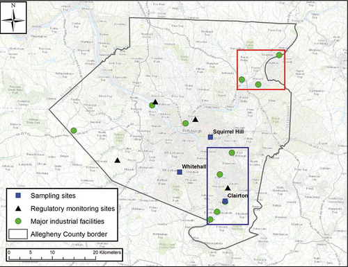
The goals of this study were to (1) measure air toxics exposure with high time resolution (30 min) in two residential neighborhoods located far (>10 km) from the major industrial source regions of HAPs in Allegheny County, (2) attribute exposure of measured air toxics to sources, (3) determine the spatial extent of industrial plume impacts, and (4) investigate the potential for exposure misclassification using data collected at long time resolutions (e.g., 2-week aggregated samples) relative to high time resolution data.

Methods

Sampling locations and measurements

Measurements of a suite of VOCs, including air toxics, and particulate black carbon (BC) were conducted at three locations in the Pittsburgh metro area, as indicated in Figure 1. The Clairton site (40°17’45.3” N, 79°52’29.4” W) was located on a residential street in the Monongahela River valley approximately 1 km south of a large metallurgical coke oven and in close proximity to several other major industrial sources. Measurements were conducted from June 3 to July 22, 2014. The Whitehall site (40°21’15.6” N, 80°0’1.8” W) was located in a suburban residential neighborhood, 12 km northwest of the Clairton site and 10 km south of downtown Pittsburgh. Measurements were conducted from June 5 to June 30, 2014. Following completion of the measurements at the Whitehall site, the measurement station was moved to the Squirrel Hill site (40°25’44” N, 79°55’7.5” W). This site was in a residential neighborhood 14 km north-northwest of the Clairton site and 7 km east of downtown Pittsburgh, and sat on a hilltop overlooking the Monongahela River valley. Measurements were conducted from July 1 to July 15, 2014.

BC was measured at all three sites using a multi-angle aerosol absorption photometer (MAAP; Thermo Scientific model 5012). The MAAP a converts absorption coefficient measurements at a wavelength of 670 nm to BC mass using a mass absorption cross-section (MAC) value of 6.6 m² g⁻¹ (Petzold et al., 2002).

A suite of VOCs was measured with one of two semicontinuous gas chromatographs with flame ionization detection (GC-FID; Airmo model GC 866 at Clairton and SRI model 8610 at Whitehall and Squirrel Hill). Each GC used an activated carbon trap to preconcentrate ambient samples before thermal desorption and injection into the GC column. The two GC-FIDs operated on identical 30-min cycles. Table S1 (supplemental data) outlines the GC-FID sample and analysis cycles. The Airmo GC in Clairton was unavailable from June 7 to July 9 due to a maintenance issue.

Quantified VOCs range from C₄ to C₁₂ linear and branched hydrocarbons, single-ring aromatic species (e.g., benzene, toluene, xylene isomers, trimethyl benzene isomers), and oxygenated VOCs (Table S2, supplemental data). Both GC-FIDs were calibrated and retention times for species of interest were measured with an authenticated gas mixture at the start and end of the measurement campaign. Additionally, the Airmo GC ran an autocalibration cycle with an internal benzene standard once per day.

GC chromatograms were analyzed using the Matlab ipeak function after baseline correction. Peaks appearing in at least 50% of the chromatograms collected at Whitehall and Squirrel Hill were quantified. Twenty such peaks were identified (Table S2, supplemental data). Of these 20 peaks, nine were positively identified based on retention time (Table 1 and S2). Three peaks corresponding to C₆ hydrocarbons, C₉ hydrocarbons, and C₅ carbonyl(s) were identified by retention time, but specific isomers could not be identified. The C₆ and C₉ hydrocarbons were quantified based on the corresponding n-alkane as a calibration standard and the C₅ carbonyl was quantified using 2-pentanone as the calibration standard. The remaining eight peaks were unidentified. Concentrations of these unidentified species were estimated using the average response factor of the identified species.

Table 1. Concentrations (mean, median, 25th, 75th, and 95th percentiles) of identified species measured at Whitehall and Squirrel Hill.

	Whitehall					Squirrel Hill					Logue et al. (2009b)
	Mean	Median	25th	75th	95th	Mean	Median	25th	75th	95th	Downtown	CMU
Black carbon	0.82	0.59	0.41	1.01	1.95	1.04	0.58	0.17	1.67	3.91
Acetone	0.35	0.35	0.26	0.42	0.53	0.35	0.32	0.24	0.44	0.56
C6 hydrocarbons*	0.35	0.33	0.25	0.43	0.70	0.33	0.29	0.21	0.43	0.75
C5 carbonyl*	1.33	1.08	0.76	1.58	2.93	0.42	0.39	0.29	0.50	0.85
Heptane	0.24	0.19	0.13	0.30	0.54	0.17	0.15	0.00	0.23	0.47	1.36	0.96
Toluene	1.20	0.88	0.56	1.62	3.01	1.05	0.70	0.51	1.08	3.62	1.49	0.63
C9 hydrocarbons*	0.16	0.14	0.00	0.20	0.41	0.10	0.00	0.00	0.16	0.30
m+p-Xylene	0.82	0.61	0.45	1.03	2.04	0.69	0.50	0.37	0.76	2.21	0.93	0.14
o-Xylene	0.27	0.16	0.00	0.31	0.88	0.25	0.15	0.00	0.26	1.01	0.67	0.10
1,3,5-Trimethyl benzene	0.21	0.16	0.00	0.32	0.64	0.16	0.00	0.00	0.20	0.79	0.00	0.04
1,2,4- Trimethyl benzene	0.35	0.23	0.15	0.42	0.87	0.24	0.16	0.00	0.27	0.96	0.14	0.14
1,2,3- Trimethyl benzene	0.30	0.27	0.17	0.41	0.64	0.07	0.00	0.00	0.14	0.28

Note: Species indicated with an asterisk were tentatively identified but specific isomers could not be confirmed. Median concentrations measured by Logue et al. at two sampling locations are also included. All concentrations are in μg m⁻³.

During daylight hours the secondary C₅ carbonyl (retention time = 340 sec) interfered with, and was often larger than, the benzene peak (retention time = 357 sec) in the chromatogram. Therefore, benzene concentrations for Whitehall and Squirrel Hill are only presented for overnight hours. The m-xylene and p-xylene are not separable by the GC column and temperature program used here, and are therefore reported as the sum of the two isomers.

Figure S1 in the Supplemental data shows the wind conditions during the study period as measured at the Allegheny County Airport (airport code KAGC). Winds during the study period were typically from the south and southwest, with occasional winds from the northwest and southeast. Wind speeds during the study period were generally less than 5 miles per hour. Figure S1 compares the wind speed and direction during the measurement campaign to the annual wind speed and direction. Westerly winds were less common during the study period than over the full year, and average wind speeds were lower (1.7 mph vs. 2.9 mph).

Positive matrix factorization

Factor analysis of the combined VOC and BC data was conducted using positive matrix factorization (PMF) (Paatero and Tapper, 1994). PMF analysis used the multilinear engine (ME-2) (Paatero, 1997) as implemented in the EPA PMF version 5.0 software.

Receptor models such as PMF solve eq 1, where a data matrix x with i observations of j species is explained by a combination of P sources. Each source has a source profile (f) describing the mix of pollutant emissions from the source and source strength (mass contribution) g.

(1)

In positive matrix factorization, eq 1 is solved without any source profiles being specified. PMF minimizes the residual error (ε) and the objective function Q (eq 2), where u_ij is the measurement uncertainty of species j in sample i. Rotational ambiguity in the PMF solution is investigated using varimax rotation.

(2)

Dispersion modeling

The AERMOD dispersion model (Cimorelli et al., 2005; Perry et al., 2005) was used to simulate emissions of toluene and SO₂ from major point sources identified in Allegheny and surrounding counties. Table S3 (supplemental data) lists the modeled sources, their locations, and SO₂ and toluene emission rates. Annual emissions for 2013 were obtained from Pennsylvania Department of Environmental Protection (DEP) reports (PA DEP, 2015). Emissions from each source were assumed to be constant throughout the year, and each source was assumed to operate 365 days per year.

Simulations were conducted with hourly resolution using 2013 meteorology. Surface and vertical profile meteorological input files for AERMOD were obtained from the Allegheny County Health Department modeling group (personal communication with J. Maranche). Meteorological data represent vector averages National Weather Service wind data, averaged to hourly resolution.

Modeled species were treated as inert tracer species, as typical photochemical losses are significantly slower than transport outside of the modeling domain. The model domain was a field of 100 receptors evenly spaced on a 54 × 45 km grid (Figure S2) that covered the southern two-thirds of Allegheny County and extended into neighboring counties. Receptor heights were specified to match actual land elevation above sea level.

Results and discussion

Data overview and identification of pollutant plume events

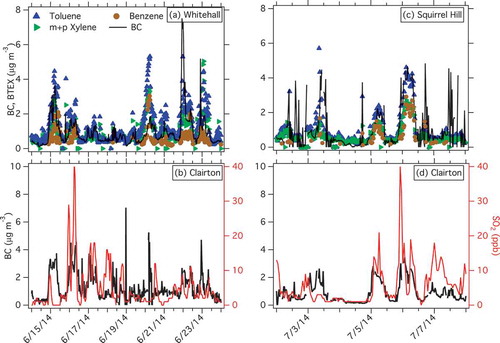
Table 1 summarizes descriptive statistics of BC and identified VOCs measured at Whitehall and Squirrel Hill. Figures 2a and 2c show typical time series for BC, benzene (overnight only), toluene, and m+p-xylene from the Whitehall and Squirrel Hill sites. Figures 2b and 2d show BC measured in Clairton (study mean = 0.99, median = 0.71, interquartile range [IQR] = 0.84 μg m⁻³) and SO₂ measured by the EPA AQS at a monitoring station located 3 km from the Clairton measurement site during time periods concurrent to the Whitehall and Squirrel Hill measurements.

Figure 2. Time series of BC, toluene, m+p-xylene peaks, and benzene (overnight hours only) measured at Whitehall (a) and Squirrel Hill (c). Panels (b) and (d) show BC measured in Clairton and SO₂ measured by the EPA AQS near Clairton during the same time periods as the Whitehall and Squirrel Hill measurements.

Median concentrations of BC and BTEX species at Whitehall and Squirrel Hill are similar (e.g., median BC ~0.6 μg m⁻³), and consistent with each site being located far from major sources or roadways and representative of the urban background in Allegheny County. In a series of measurements conducted during 2011–2013, Tan et al. (2014a) reported that the median BC concentration in urban and suburban background areas in Allegheny County is approximately 0.5–0.6 μg m⁻³, with higher concentrations in high traffic and industrial dominated areas. Likewise, median toluene concentrations at both Whitehall and Squirrel Hill fall in the bottom quartile of concentrations reported by Tan et al. (2014a), consistent with the sites representing urban/suburban background concentrations.

Table 1 also lists VOC measurements from Logue et al. (2009b) at traffic-dominated (downtown Pittsburgh) and urban background (Carnegie Mellon University campus; CMU) measurement sites. The data collected at the Whitehall and Squirrel Hill sites typically fall within the range bounded by the Logue et al. data. Specifically, concentrations of toluene, m+p-xylene, and o-xylene measured at Whitehall and Squirrel Hill were higher than measurements by Logue et al. at CMU but lower than the downtown Pittsburgh measurements. One notable exception to this trend is heptane, which had concentrations a factor of 5–7 lower in the current study. The similarity in BTEX concentrations measured here and by Logue et al. suggests that countywide emissions of these species have not changed substantially in the past ~10 years, which is reflected in the emissions inventory (Kelly and Fischman, 2011).

At Whitehall and Squirrel Hill, concentrations of BC and the BTEX species show a pattern of nighttime maxima, with concentrations typically peaking between midnight and 6 a.m. (all times are local time). This is shown in Figure 2. Typical daytime concentrations for BC, m+p-xylene, and toluene are approximately 0.4–1 μg m⁻³. During the overnight hours, concentrations of these species rise to 1.5–6 μg m⁻³ for periods of 6–12 hr. While these pollutants all show a similar temporal pattern, especially at night, there are day-to-day variations in pollutant ratios (e.g., toluene/BC), suggesting that multiple emissions sources might impact the sampling sites.

Overnight peaks in BTEX and BC at Squirrel Hill and Whitehall are accompanied by concurrent peaks in BC and SO₂ in Clairton, as shown in Figure 2. GC data collected at Clairton outside of the time window shown in Figure 2 indicate that BTEX species also peak during overnight periods when BC and SO₂ peak. These concurrent multipollutant peaks can plausibly be caused by one of two factors: transport of upwind emissions into the sampling domain (e.g., via weather patterns), or local emissions trapped low to the ground by temperature inversions. As discussed in the following, the latter is the more likely explanation.

If the overnight peaks in pollutant concentrations were the result of upwind emissions transported into the sampling domain, one would expect to observe perfect correlation between plumes at Clairton and either Whitehall or Squirrel Hill. Additionally, SO₂ measured by the regulatory network would peak both in Clairton and at other monitors in the county. This is not the case. BC and SO₂ peaks are regularly observed in Clairton without a concurrent peak at Whitehall or Squirrel Hill (e.g., June 17–18, July 17). Additionally, the other SO₂ monitors located in the county do not always display concurrent peaks with the monitor shown in Figure 2. The occurrence of pollutant maxima in Clairton but not in nearby communities is one indication that the overnight peaks result from local industrial emissions.

Atmospheric soundings (Figures S3 and S4) provide evidence that the plumes are the result of local emissions trapped near ground level by inversions. Overnight peaks in BC and BTEX observed in this study occurred exclusively during periods of low mixing height. For example, the large plume event observed on June 20 coincided with a strong inversion with a mixing height below the 950-mbar level (<~500 m above ground level). In contrast, no plume event was observed on July 4 when the there was a weak temperature inversion aloft and the mixing height was approximately 1000 m above ground level. Over the course of the study period, elevated nighttime pollutant concentrations coincided with temperature inversions and low mixing height. These conditions were met on approximately 33% of nights during the sampling period.

PMF and factor identification

PMF was used to identify the sources of BC and VOCs observed at the receptor sites. All of the data collected at Whitehall and Squirrel Hill were analyzed as a single data set in order to determine a consistent set of factors (sources) between the two sites. Due to daytime interference problems described earlier, benzene was not included in the PMF analysis. The estimated concentrations of the eight unidentified peaks in the GC chromatograms (Table S2) were included in PMF analysis to assist in resolving as many relevant sources as possible.

Figure 3 shows a five-factor PMF solution and the accompanying apportionment of m+p-xylene for the period of June 14–24 at Whitehall. The five factors are gasoline vehicles, diesel vehicles, industrial emissions, a secondary factor, and a secondary/area sources factor. For the full study period at Whitehall and Squirrel Hill, the five-factor solution describes 98 ± 10% of the measured concentrations of m+p-xylene. Table S2 in the Supplemental data summarizes the PMF solution.

Figure 3. Five-factor PMF apportionment of m+p-xylene measured at Whitehall. The pie charts at the right show the contributions of each factor to m+p-xylene and toluene for the entire set of measurements at Whitehall and Squirrel Hill.

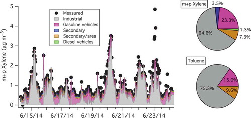
Figure 3 also shows the study-wide apportionment of m+p-xylene and toluene to the five PMF factors. The industrial and gasoline vehicle factors account for approximately 90% of the total mass for each compound. The overnight plumes are assigned almost entirely to the industrial factor that contributes approximately 70% of both the observed toluene and m+p-xylene concentrations.

PMF solves eq 1 without specifying any source profiles a priori. Thus, one challenge in applying PMF to ambient data sets is to identify the factors and assign them to specific emissions sources. In the subsequent sections we describe each of the five factors and use several tools to assign the factors to sources, including ratio-ratio plots, diurnal patterns, and wind direction patterns.

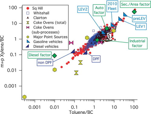
Ratio–ratio plots were introduced by Robinson et al. (2006a, 2006b, 2006c, 2006d) to visualize the mixing of multiple sources and photochemical aging of molecular markers in source apportionment studies. Mixing between multiple sources can be described by drawing mixing lines or mixing regions between the sources. Figure 4 shows a ratio–ratio plot for toluene and m+p-xylene, both normalized by BC, for data collected at the three sampling sites. The ambient data organize roughly along a line between (0.01, 0.01) and (100, 100). The overlap between data collected at the three sampling sites suggests that all three sites are impacted by a common set of sources. The ratio–ratio plot indicates that these three pollutants can be described by mixing of two or more factors. Mixing lines drawn between the factors should bound the ambient data.

Figure 4. Ratio–ratio plot of m+p-xylene and toluene, each normalized by BC. Data collected at Clairton, Squirrel Hill, and Whitehall organize along a single line, suggesting that the same sources are important at each site. PMF factors are shown as green diamonds. Total annual emissions profiles from industrial facilities indicated in Figure 1 are shown, as well as emission profiles from subprocesses associated with metallurgical coke ovens.

Gasoline and diesel vehicle factors

PMF revealed two factors related to traffic, one each for gasoline and diesel vehicles. The gasoline vehicle factor describes 15% of toluene, 23% of m+p-xylene, and 5% of BC. The diesel vehicle factor accounts for 16% of the measured BC but only about 1% of m+p-xylene and contributes negligibly to toluene.

The gasoline vehicle factor shows strong agreement with both published emissions for gasoline vehicles and the expected fleet composition. Figure 4 shows that the gasoline vehicle factor lies along a mixing line defined by source profiles of a series of vehicles tested by May et al. (2014). The vehicles are classified according to the California low emission vehicle (LEV) program. The oldest vehicles (pre-LEV; model years before 1994) have the highest emissions of BTEX species, and newer LEV-1 (1995–2002) and LEV-2 (2003–2013) vehicles have progressively lower BTEX emissions. BC emissions were roughly constant across the model years, and thus the m+p-xylene/BC and toluene/BC ratios decrease for newer vehicles.

Figure 4 also shows a fleet average emission profile built using Allegheny County vehicle miles traveled and model year data for 2010. LEV-1 and LEV-2 vehicles dominated the 2010 vehicle fleet, with roughly equal miles traveled by vehicles in each class. Thus, the 2010 fleet emissions profile lies approximately halfway between the LEV-1 and LEV-2 source profiles. The gasoline vehicle factor identified by PMF falls between the 2010 fleet and the LEV-2 source tests, consistent with the 2014 on-road fleet containing more LEV-2 vehicles and fewer LEV-1 and pre-LEV vehicles.

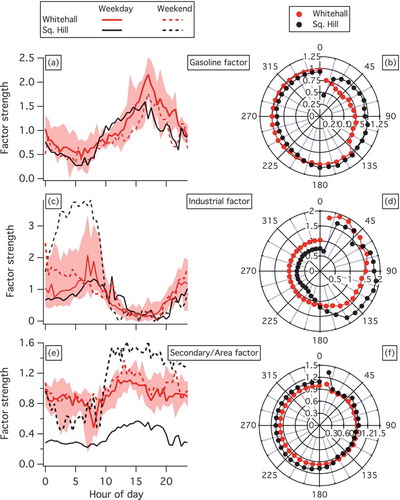
Figure 3 shows that the contribution of the gasoline vehicle factor to measured m+p-xylene concentrations is low at night and higher in the day, as would be expected based on traffic patterns. Figure 5a shows diurnal patterns for the gasoline vehicle factor strength on weekdays and weekends. The diurnal and weekly patterns match well with expected traffic patterns. Specifically, there is a 20–25% reduction in factor strength on weekends that matches well with overall weekday–weekend traffic patterns for gasoline vehicles in the United States (McDonald et al., 2013). The factor strength peaks at 5 p.m., reflecting the sampling locations in residential neighborhoods—the peak results from commuters returning home for the evening. The overall diurnal trend of the factor strength, including the afternoon peak, is also consistent with the traffic volumes measured in a nearby highway tunnel (Figure S5) that many commuters traverse during their afternoon commute.

Figure 5. Diurnal patterns and wind dependence of PMF factor strengths for gasoline vehicles (panels (a) and (b)), industrial emissions (panels (c) and (d)), and secondary/area factor (panels (e) and (f)). Lines in panels (a), (c), and (e) show median factor strengths. Shaded areas in panels (a), (c), and (e) show the interquartile range for weekday measurements at Whitehall. The wind roses in panels (b), (d), and (f) represent average factor strengths segmented into 10º bins.

The gasoline vehicle factor does not display a morning rush-hour peak, though one might be expected based on traffic activity data, especially on weekday mornings. Automobile emissions are highest during cold starts (May et al., 2014)—the first few minutes of vehicle operation—and concentrations of some vehicle-related pollutants such as NO and particle-bound polycyclic aromatic hydrocarbons are highest in the morning rush hour in Pittsburgh (Tan et al., 2014a). It is not clear why a morning peak is not observed in the gasoline PMF factor in this data set.

Figure 5b shows the gasoline vehicle factor strength as a function of wind direction at both Whitehall and Squirrel Hill. The factor strength shows almost no dependence on wind direction for the Squirrel Hill site. This suggests that the measurements are not strongly influenced by emissions from a particular nearby highway or vehicles traveling on the residential street outside the sampling site. It further suggests that roadways are more or less evenly distributed around the site, which is indeed the case. The gasoline factor strength was approximately 25% weaker at Whitehall when winds came from the east. This is consistent with the distribution of roadways around the site, as a large golf course is located 1 km east of the Whitehall site.

The diesel vehicle factor exhibits reasonable agreement with published emissions profiles. Both modern diesel vehicles equipped with diesel particulate filters (DPF) and older diesel vehicles (pre-2007, “non-DPF”) emit significantly more BC than BTEX (Figure 4) (May et al., 2014; Schauer et al., 1999). The diesel vehicle factor identified here has an m+p-xylene/BC ratio similar to emissions tests of diesel vehicles, but is depleted in toluene relative to the source tests.

The diurnal pattern of the diesel factor (Figure S6) exhibits a morning maximum between 4 and 6 a.m. and an afternoon minimum from 3 to 5 p.m. As with the gasoline factor already described, this pattern matches well with diesel vehicle traffic patterns measured in a local traffic tunnel. As a function of the total on-road fleet, diesel vehicles reach a minimum during the afternoon rush hour. The diesel vehicle factor shows wind direction dependence similar to that of the gasoline vehicle factor, reflecting a similar source region (e.g., the road network).

Secondary and area factors

PMF identified two factors associated with secondary species; we assign one as a purely secondary factor and the other as a mixed secondary/area sources factor. The secondary factor has the C₅ carbonyl as the most abundant species (Table S2). Both this species and the factor display a clear photochemical origin. Concentrations are low overnight, steadily increase during daylight hours, and peak around sunset (Figure S6). The day/night ratio of factor strengths is 2. Additionally, this factor shows no wind direction dependence, suggesting a regional secondary origin.

PMF also identified a factor that includes both secondary species (acetone) and primary pollutants such as toluene, heptane, and BC. This factor is identified as being a secondary/area sources factor. It describes a small fraction of BC (<1%) and BTEX species (<5%). Figure 4 shows that this species defines the upper rightmost point of the ratio-ratio plot, indicative of a source that has much higher aromatic VOC emissions than BC emissions.

The diurnal pattern for this factor (Figure 5e) shows a modest afternoon maximum, with the source strength in the afternoon only about 10% higher than in the morning. There is not a strong weekday–weekend pattern, which rules out common primary sources such as traffic. The factor strength is nearly independent of wind direction, with a 10% reduction in factor strength for winds from the east versus winds from the west.

This factor may therefore represent widely distributed area sources, such as fuel evaporation, which would be dominated by VOCs with very little BC. It may also represent a combined source, not completely resolved by PMF into separate sources, that incorporates secondary species with temperature-driven area emissions. This factor may also represent regional background concentrations.

Industrial factor

The factors discussed in the preceding account for approximately one-quarter to one-third of the BTEX and BC measured at Whitehall and Squirrel Hill. The remaining contribution comes primarily in the form of the overnight plume events attributed to industrial emissions (Figure 3).

Figure 5c shows the diurnal trend for the source strength of the industrial factor. The mean diurnal pattern exhibits a daytime minimum and an overnight maximum peaking at approximately 5–6 a.m. Figure 5c shows large weekday–weekend differences in the factor strength at Squirrel Hill; these differences are driven by large plume events that occurred on consecutive weekends and weaker plume events on weekday nights. Such night-to-night variability in plume impacts is evident in the measurements (Figures 2 and 3).

Figure 5d shows the wind pattern for the industrial factor strength, and indicates a clear geographic pattern. The strength of the industrial factor is larger for wind directions between 15° and 145°. There are numerous point sources upwind of the sampling sites, with many concentrated in the Monongahela River and Allegheny River valleys, as shown in Figure 1. The wind pattern in Figure 5d suggests that these source regions contribute to the observed overnight pollutant plumes at the receptor sites.

Unlike the gasoline or diesel vehicle factors, the industrial factor cannot be linked directly to a single source. Thus, attributing the specific source(s) of the industrial emissions factor poses a significant hurdle to interpreting the PMF results. Figure 4 shows the PMF-derived industrial source profile as well as emissions profiles from nearby point sources as determined from reports to the Pennsylvania Department of Environmental Protection (PA DEP, 2015). None of the individual point sources show the same close agreement with the PMF industrial factor as does, for example, the gasoline vehicle factor and source test emissions described earlier. The industrial factor more likely represents an aggregation of multiple sources clustered in close geographic proximity.

Emissions profiles for industrial sources shown in Figure 4 represent total annual emissions from these sources. However, many industrial sources are composed of multiple subprocesses, with unique emissions for each subprocess. For example, metallurgical coke ovens are major emissions sources in Pittsburgh (Robinson et al., 2006b; Subramanian et al., 2006). The overall coke oven emissions profiles are dominated by BC, and thus toluene/BC and m+p-xylene/BC ratios in Figure 4 are less than 1 for these sources. However much of the BC is emitted by subprocesses that do not emit BTEX. Similarly, the specific subprocesses that emit most of the BTEX emit little BC (Kelly and Besselman, 2007; Kelly and Fischman, 2011). Therefore, the overall emission profile for a particular source may be a poor indicator for the expected, temporally varying, downwind concentration profiles and subsequent factors derived by PMF.

Example profiles of the two coke oven subprocesses that emit the majority of toluene (by-products recovery and door leaks) are plotted in Figure 4. One of these subprocesses (by-products recovery) has a source profile very similar to the PMF industrial factor. However, without more detailed information about time–activity patterns at these facilities, it is nearly impossible to correlate the observed plumes to specific subprocesses at industrial facilities.

Dispersion modeling of industrial sources

The analysis of PMF factors presented in Figures 3–5 suggests that industrial plumes dominate BTEX concentrations at the measurement sites. The wind direction patterns in Figure 5c further suggest that the overnight BTEX plumes arise from clusters of sources in the Allegheny and Monongahela river valleys. However, as described earlier, PMF only identifies factors, not specific sources, and uncertainty exists surrounding the identity of the industrial factor. Thus, we also used dispersion modeling to investigate source impacts in the sampling domain.

Figure 6 presents results of AERMOD dispersion modeling of toluene concentrations for the Whitehall sampling site. Figure 6a shows a time series of predicted toluene concentrations resulting from emissions from major industrial sources (Table S3) for 2013. Numerous plume events are visible, with most predicted to occur during overnight hours. We define a plume event to occur on a day if at least one hour has a predicted concentration above the 95th percentile for the entire simulated year. This condition was met on 146 days (40%).

Figure 6. Modeled concentrations of toluene at the Whitehall site predicted by AERMOD using 2013 meteorology and modeled at hourly resolution. (a) A time series of predicted concentrations for Julian days 119–129 (May 29–June 9). The inset shows the full year of simulated concentrations. (b) The mean diurnal pattern predicted by AERMOD (red/darker line) and the diurnal pattern of toluene concentrations derived from the PMF-derived industrial factor (gray/lighter line; divided by 10). (c) Toluene concentrations segmented into 10º bins for AERMOD (red/darker line) and determined from the PMF industrial factor (gray/lighter line; divided by 10).

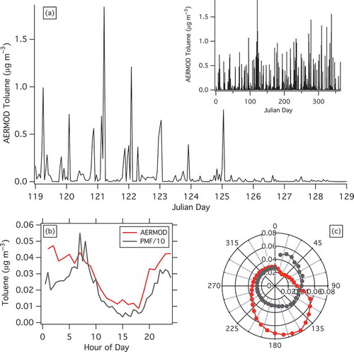
There is qualitative agreement between AERMOD predictions and the observed toluene concentrations (Figure 2). Both AERMOD and the measurements indicate overnight high concentration events peaking between midnight and 6 a.m.. The resultant diurnal pattern of modeled toluene (Figure 6b) exhibits an overnight maximum and midday minimum. However, the magnitude of individual plume events is significantly different, with AERMOD predicting lower concentrations than the measurements. Many predicted plumes shown in Figure 6a have a maximum concentration between 0.5 and 1.5 μg m⁻³, whereas the data shown in Figure 2 suggest that overnight plumes frequently reach 2–4 μg m⁻³.

Figure 6c shows a wind rose of predicted toluene concentrations. Predicted toluene concentrations peak when winds arrive at the receptor site from the south-southeast. Thus, the wind direction dependence suggests the influence of sources in the Monongahela River valley. AERMOD does not predict plume impacts to occur when winds arrive from more northeasterly wind vectors.

Comparison of dispersion model and PMF: Industrial sources

There are several areas of qualitative agreement between the AERMOD dispersion model results and PMF, but quantitative agreement is lacking. Both AERMOD and PMF identify industrial plumes during overnight hours, but the magnitude of these plumes differs significantly. As described earlier, concentrations during individual plume events predicted by AERMOD are at least a factor of 2–3 smaller than observed overnight plumes. When aggregated over a diurnal cycle, PMF and AERMOD differ by an order of magnitude. The average diurnal patterns in Figure 6b show the same overall shape, with higher concentrations overnight and daytime minima, but with a factor of 10 higher concentration attributed to industrial sources by PMF.

AERMOD and PMF suggest different source regions for the industrial plumes (Figure 6c). The PMF industrial factor indicates that plumes can arrive from a wide range of upwind directions, suggesting that sources in both the Allegheny and Monongahela river valleys strongly impact the receptor site. AERMOD only identifies plumes arising from the Monongahela River valley as having a significant impact on the modeled receptor site.

We postulate three explanations for the discrepancies between AERMOD and PMF in identifying industrial source impacts: (1) overapportionment of industrial sources by PMF; (2) missing or underestimated emissions from the modeled sources in AERMOD; and (3) inaccuracies in pollutant dispersion predicted by AERMOD in a challenging valley environment and/or under low wind speeds. These are addressed in turn.

PMF separates the observed concentrations into factors through a combination of compositional (e.g., toluene/BC ratio) and temporal variations. Thus, sources or phenomena that are degenerate in either composition or temporal pattern can be difficult to segregate. In the context of this study, the PMF industrial factor may convolve regional background concentrations with industrial plumes. Background pollutant concentrations are expected to follow the general pattern of higher overnight concentrations and lower daytime concentrations, driven primarily by changes in the boundary layer height. Convolving industrial emissions with the regional background would further require that the emissions have a similar composition as the regional background. In this region with high BTEX emissions, that may be plausible.

If PMF cannot separate industrial emissions from the regional background, it would have the effect of over stating the influence of industrial emissions at the receptor sites. We tested this possibility by adding additional factors to PMF. While this did not change industrial apportionment significantly, we cannot entirely rule out the possibility that the industrial factor describes at least a portion of the regional background, as indicated by the nonzero factor strength for westerly wind directions in Figure 5d.

The concentrations predicted by AERMOD may be lower than PMF determinations of industrial impacts because of missing sources or under estimated emissions from known sources. The dispersion model relies upon reported emissions from individual facilities as inputs (Figure S3). While emissions of some species, typically criteria pollutants, are directly measured with real-time stack monitors, other emissions are estimated from engineering calculations (Kelly and Besselman, 2007; Kelly and Fischman, 2011). This introduces the possibility that reported emissions of BTEX species such as those modeled here may be in error.

There are numerous instances of underreported emissions in inventories (Hu et al, 2015), including some large discrepancies (Brandt et al., 2014). However in order for AERMOD predictions to match with the PMF analysis, emissions would have to be under reported by roughly a factor of 10 (e.g., Figure 6b). This seems unlikely.

AERMOD may also predict low concentrations because of missing sources. The dispersion modeling here (Figure 6 and Table S3) accounts for all major toluene sources that report emissions. The modeling does not account for widely distributed smaller sources (e.g., gas stations) or area sources. While these may be important emissions sources, emissions from gas stations, or other ubiquitous sources, would not be expected to produce the observed spatial pattern in the PMF wind rose.

The terrain in the modeling domain poses a challenge to using AERMOD or other dispersion models. The modeling domain is characterized by a broad plateau cut by deep river valleys. The river valley is, on average, 100 m below the surrounding plateau (Allegheny County—Contours, 2006). Many of the industrial sources are located in the river valleys. AERMOD uses a single surface wind speed and direction to characterize the entire sampling domain. This value is obtained from meteorological measurements conducted at an airport located on the plateau. Wind speed and direction in the river valley can differ significantly from the more regional winds measured on the plateau (Butler et al., 2015). This can introduce errors into the concentrations predicted by AERMOD or other dispersion models.

An additional limitation in comparing PMF and AERMOD results may be the limited time window of the measurements, which cover roughly 1 month in the summer. The short duration of the measurements may create biases in determining annual average concentrations and plume frequency for the measurement sites (Tan et al., 2014b). However, limiting the PMF versus AERMOD comparison only to the months of June and July does not substantially improve agreement.

The quantitative disagreement between PMF and AERMOD complicates the attribution of population exposures due to these plumes. However, while the magnitude of these plume impacts is uncertain, both PMF and AERMOD results presented here suggest that industrial plumes can spread over a large area. These plumes can impact areas both near the major source regions, as well as areas up to 10–15 km down wind of the source region (Figure S7).

Averaging time effects

As described earlier, a common method for determining annual-average exposures to pollutants is to deploy samplers that collect integrated 1- or 2-week samples. For example, both the ESCAPE and NYCCAS studies used 2-week passive samples of NO₂ and integrated PM_2.5 filter samples spread over multiple seasons to determine annual-average exposures. Long-term integrated samples are attractive for numerous reasons, including low cost and ease of deployment, especially for regulatory bodies or health departments looking to evaluate exposures in a particular community where a real-time monitor is not operating. However, in a region such as Pittsburgh, where subdaily industrial plumes can impact communities, the use of integrated samplers can lead to exposure misclassification and underestimation of industrial source plume impacts.

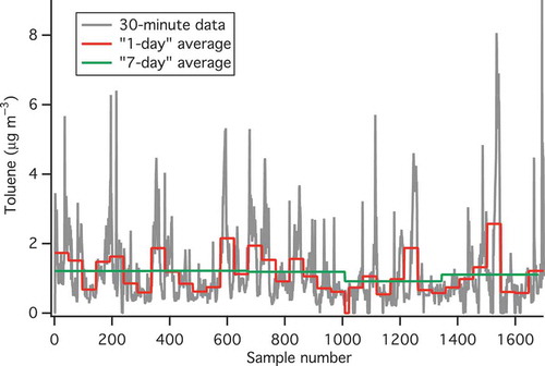
An example of potential exposure misclassification is shown in Figure 7, which compares the 30-min toluene measurements collected at Whitehall and Squirrel Hill (shown as a single, continuous time series), to two longer term averages. One-day (48 consecutive samples) and 7-day (336 consecutive samples) averages were calculated from the 30-min data. As discussed earlier, the 30-min data show clear, subdaily plumes associated with industrial emissions (mean = 1.13 μg m⁻³, median = 0.80 μg m⁻³, IQR = 0.87 μg m⁻³). The 1-day averages lose much of this temporal fidelity, and averaging over plume events increases the median concentration by 20% (median = 0.98 μg m⁻³, IQR = 0.84 μg m⁻³). The 1-day pseudo samples can be used to distinguish days with “higher” versus “lower” concentration, driven primarily by the presence or lack of an overnight plume.

Figure 7. Toluene concentrations represented over three different averaging times. The grey line shows the raw data at 30-min resolution. The red line shows a 1-day average concentration constructed by averaging 48 consecutive 30-min measurements. The green line shows a 7-day average constructed from 336 consecutive measurements.

PMF analysis of the 1-day pseudo samples yielded a three-factor solution with traffic, industrial, and secondary factors. There was insufficient variability in the 1-day samples to extract separate gasoline and diesel factors or multiple secondary factors. The gasoline and diesel factors in the five-factor PMF solution described earlier (Figures 3, 4, and 5) are separated in part by differences in the diurnal trend; therefore, daily average samples obscure this variability.

The industrial factor determined for the 1-day pseudo samples contributed 50% of the toluene and m+p-xylene, with the remainder attributed to the traffic factor. Thus, the longer sampling time leads to a substantial misapportionment of BTEX relative to the 30-min data, with the specific impact of under estimating the impact of subdaily plume events to the overall exposure and nearly doubling the exposure attributed to traffic.

The 7-day average shows very little variation, with a nearly constant concentration (mean = 1.13 μg m⁻³, median = 1.19 μg m⁻³, IQR = 0.11 μg m⁻³) over the study period. An acceptable PMF solution was not reached for the 7-day samples, as there was insufficient variation in the data to determine separate factors. Thus BTEX exposure in the 7-day samples cannot be attributed to specific source classes using PMF. In this case, using a typical 1-week or 2-week integrated sample would not be capable of informing BTEX or BC exposure associated with industrial plumes.

The averaging time analysis in the preceding relies on the PMF interpretation of the data, which suggests that industrial plumes are the dominant source of BTEX exposures. However, if the AERMOD results are correct and plume impacts are approximately 10 times smaller than predicted by PMF, the discrepancy introduced by longer term average samples is reduced. Regardless of the source of the subdaily high-concentration events (e.g., industrial emissions vs. changes in the regional background), the aggregated samples do not capture the full dynamic range of concentrations at the receptor site, nor can the time series of aggregated samples be fully resolved into different source factors.

Discussion and wider applicability

Taken alone or in concert, exposures to BTEX species measured in this study may not pose an acute or chronic health risk. None of the species measured here exceeded minimum risk levels established by the U.S. Agency for Toxic Substances and Disease Registry (ATSDR) for chronic or acute exposure. Nor do they exceed chronic cancer risk levels from the EPA Integrated Risk Information System (IRIS).

Logue et al. (2009a) previously measured BTEX species at several locations in Pittsburgh and found that benzene was the only locally emitted VOC to exceed a cancer lifetime incidence rate (LIR) of 10⁻⁵. Logue et al. also considered noncancer effects, and again benzene exhibited the highest hazard quotient (5 × 10⁻²) of any VOC quantified here. Concentrations of BTEX species measured in this study are similar to those measured by Logue et al. (Table 1). Thus, the results presented here are consistent with the findings of Logue et al in two important aspects: (1) BTEX and other VOCs, particularly those emitted from industrial sources, do not appear to be major drivers of chronic cancer risk in Allegheny County, and (2) nonmobile sources are important contributors to overall BTEX exposure in Allegheny County.

While the concentrations of BTEX species measured here do not exceed ATSDR or IRIS chronic risk levels, the concentrations may still be sufficient to trigger health endpoints. A recent review by Bolden et al. (2015) indicates that BTEX species can have endocrine disrupting properties at concentrations below the IRIS limits. Bolden et al. list minimum effect concentrations for long-term exposures to benzene (1.01 μg m⁻³), toluene (6.95 μg m⁻³), and m+p-xylene (4.1 μg m⁻³), as well as respiratory impacts of short-term benzene exposures at concentrations greater than 1.5–2 μg m⁻³. Both the chronic and short-term minimum effect concentrations for benzene were routinely exceeded during plume events (Figure 2). While the chronic minimum effect concentrations for toluene or m+p-xylene were not exceeded at Whitehall or Squirrel Hill during this study, these limits were exceeded at the Clairton sampling site during plume events.

While the plumes are predicted to impact a wide area, a complication arises in assigning exposure from these plumes. As described earlier, the PMF industrial factor assigns a factor of 10 larger exposures to industrial factors than AERMOD dispersion modeling. Whether PMF is overapportioning industrial impacts or AERMOD is underapportioning them, the data show clear and large variations on subdaily timescales.

The results presented here also show that long-term (e.g., 1- or 2-week) average samples can misapportion population exposures in areas with significant impact by industrial emissions. Our results further suggest that high time resolution tools—either measurements or models—can identify areas where these plume impacts may be significant and could cause biases or misapportionment in long-term average samples.

A recommendation for future pollutant mapping or exposure studies would be to conduct high time resolution measurements either prior to the deployment of integrated samplers or concurrently with them in order to quantify potential plume impacts. While postcorrecting integrated samples to account for subdaily plume impacts seems unlikely, high time resolution measurements and subsequent analysis could bound the potential impacts of plumes on the measurements, as well as help define the full dynamic range of concentrations observed at the distributed monitoring locations.

Alternatively AERMOD or another dispersion model could be used to map potential extents of plume impacts (e.g., Figure S7). Such a map could identify areas where plume impacts would be expected to be important, and therefore define locations where high time resolution measurements would present more value. Dispersion modeling can also be used to identify areas where additional distributed samples could be collected with novel sampling protocols. For example, separate “plume-focused” samples (e.g., midnight–6 a.m.; Schmool et al., 2014) could be co-located with samplers aimed at annual-average concentrations (e.g., 15 min every hour) in areas where plume impacts are expected to be important.

Funding

This work was funded by the Heinz Endowments under grant E2033. The authors thank Jason Maranche of the Allegheny County Health Department for assistance with AERMOD, and Marie Kelly of the Allegheny County Health Department for assistance with the emissions inventory data for Allegheny County.

Notes on contributors

A.A.P., T.R.D., and P.G. collected data. U.R. and A.A.P. ran AERMOD simulations. A.A.P. and P.G. analyzed data. A.A.P. wrote the paper.

Supplemental data

Supplemental data for this paper can be accessed at the publisher’s Web site.

Additional information

Funding

This work was funded by the Heinz Endowments under grant E2033. The authors thank Jason Maranche of the Allegheny County Health Department for assistance with AERMOD, and Marie Kelly of the Allegheny County Health Department for assistance with the emissions inventory data for Allegheny County.

Notes on contributors

Albert A. Presto

Albert A. Presto is an Assistant Research Professor in the Department of Mechanical Engineering and the Center for Atmospheric Particle Studies at Carnegie Mellon.

Timothy R. Dallmann

Timothy R. Dallmann was a postdoc in Dr. Presto’s group and is now with the International Council on Clean Transit in Washington, DC.

Peishi Gu

Peishi Gu is a Ph.D. student and Unnati Rao was a master’s student in Dr. Presto’s group. Unnati Rao is now a student at the University of California-Riverside, Department of Chemical Engineering.

Unnati Rao

Peishi Gu is a Ph.D. student and Unnati Rao was a master’s student in Dr. Presto’s group. Unnati Rao is now a student at the University of California-Riverside, Department of Chemical Engineering.

References

- Allegheny County—Contours. 2006. ftp://www.pasda.psu.edu/pub/pasda/alleghenycounty/AlleghenyCounty_Contours2006.zip.
- Beelen, R., G. Hoek, D. Vienneau, M. Eeftens, K. Dimakopoulou, X. Pedeli, M.-Y. Tsai, N. Kunzli, T. Schikowski, A. Marcon, K.T. Eriksen, O. Raaschou-Nielsen, E. Stephanou, E. Patelarou, T. Lanki, T. Yli-Tuomi, C. Declercq, G. Falq, M. Stempfelet, M. Birk, J. Cyrys, S. von Klot, G. Nador, M.J. Varro, A. Dedele, R. Grazuleviciene, A. Molter, S. Lindley, C. Madsen, G. Cesaroni, A. Ranzi, C. Badaloni, B. Hoffmann, M. Nonnemacher, U. Kramer, T. Kuhlbusch, M. Cirach, A. de Nazelle, M. Nieuwenhuijsen, T. Bellander, M. Korek, D. Olsson, M. Stromgren, E. Dons, M. Jerrett, P. Fischer, M. Wang, B. Brunekreef, and K. de Hoogh. 2013. Development of NO2 and NOx land use regression models for estimating air pollution exposure in 36 study areas in Europe. The ESCAPE project. Atmos. Environ. 72:10–23. doi:10.1016/j.atmosenv.2013.02.037
- Bolden, A.L., C.F. Kwiatkowski, and T. Colborn. 2015. New look at BTEX: Are ambient levels a problem? Environ. Sci. Technol. 49:5261–5276. doi:10.1021/es505316f
- Brandt, A.R., G.A. Heath, E.A. Kort, F. O’Sullivan, G. Petron, S.M. Jordaan, P. Tans, J. Wilcox, A.M. Gopstein, D. Arent, S. Wofsy, N.J. Brown, R. Bradley, G.D. Stucky, D. Eardley, and R.C. Harriss. 2014. Methane leaks from North American natural gas systems. Science 343:733–35. doi:10.1126/science.1247045
- Butler, B.W., N.S. Wagenbrenner, J.M. Forthofer, B.K. Lamb, K.S. Shannon, D. Finn, R.M. Eckman, K. Clawson, L.x Wagenbrenner, P. Sopko, S. Beard, D. Jimenez, C. Wold, and M. Vosburgh. 2015. High-resolution observations of the near-surface wind field over an isolated mountain and in a steep river canyon. Atmos. Chem. Phys. 15:3785–801. doi:10.5194/acp-15-3785-2015
- Cimorelli, A.J., S.G. Perry, A. Venkatram, J.C. Weil, R.J. Paine, R.B. Wilson, R.F. Lee, W.D. Peters, and R.W. Brode. 2005. AERMOD: A dispersion model for industrial source applications. Part I: General model formulation and boundary layer characterization. J. Appl. Meteorol. 44:682–93. doi:10.1175/JAM2227.1
- Clougherty, J.E., I. Kheirbek, H.M. Eisl, Z. Ross, G. Pezeshki, J.E. Gorczynski, S. Johnson, S. Markowitz, D. Kass, and T. Matte. 2013. Intra-urban spatial variability in wintertime street-level concentrations of multiple combustion-related air pollutants: The New York City Community Air Survey (NYCCAS). J. Expos. Sci. Environ. Epidemiol. 23:232–40. doi:10.1038/jes.2012.125
- Cyrys, J., M. Eeftens, J. Heinrich, C. Ampe, A. Armengaud, R. Beelen, T. Bellander, T. Beregszaszi, M. Birk, G. Cesaroni, M. Cirach, K. de Hoogh, A. De Nazelle, F. de Vocht, C. Declercq, A. Dedele, K. Dimakopoulou, K. Eriksen, C. Galassi, R. Grazuleviciene, G. Grivas, O. Gruzieva, A.H. Gustafsson, B. Hoffmann, M. Iakovides, A. Ineichen, U. Kramer, T. Lanki, P. Lozano, C. Madsen, K. Meliefste, L. Modig, A. Molter, G. Mosler, M. Nieuwenhuijsen, M. Nonnemacher, M. Oldenwening, A. Peters, S. Pontet, N. Probst-Hensch, U. Quass, O. Raaschou-Nielsen, A. Ranzi, D. Sugiri, E.G. Stephanou, P. Taimisto, M.-Y. Tsai, E. Vaskövi, S. Villani, M. Wang, B. Brunekreef, and G. Hoek. 2012. Variation of NO2 and NOx concentrations between and within 36 European study areas: Results from the ESCAPE study. Atmos. Environ. 62:374–90. doi:10.1016/j.atmosenv.2012.07.080
- de Hoogh, K., M. Wang, M. Adam, C. Badaloni, R. Beelen, M. Birk, G. Cesaroni, M. Cirach, C. Declercq, A. Dedele, E. Dons, A. de Nazelle, M. Eeftens, K. Eriksen, C. Eriksson, P. Fischer, R. Grazuleviciene, A. Gryparis, B. Hoffmann, M. Jerrett, K. Katsouyanni, M. Iakovides, T. Lanki, S. Lindley, C. Madsen, A. Molter, G. Mosler, G. Nador, M. Nieuwenhuijsen, G. Pershagen, A. Peters, H. Phuleria, N. Probst-Hensch, O. Raaschou-Nielsen, U. Quass, A. Ranzi, E. Stephanou, D. Sugiri, P. Schwarze, M.-Y. Tsai, T. Yli-Tuomi, M.J. Varro, D. Vienneau, G. Weinmayr, B. Brunekreef, and G. Hoek. 2013. Development of land use regression models for particle composition in twenty study areas in Europe. Environ. Sci. Technol. 47:5778–86. doi:10.1021/es400156t
- Eeftens, M., R. Beelen, K. de Hoogh, T. Bellander, G. Cesaroni, M. Cirach, C. Declerq, A. Dedele, E. Dons, A. de Nazelle, et al. 2012a. Development of land use regression models for PM2.5, PM2.5 absorbance, PM10 and PMcoarse in 20 European study areas; Results of the ESCAPE project. Environ. Sci. Technol. 46:11195–205.
- Eeftens, M., M.-Y. Tsai, C. Ampe, B. Anwander, R. Beelen, T. Bellander, G. Cesaroni, M. Cirach, J. Cyrys, K. de Hoogh, A. De Nazelle, F. de Vocht, C. Declercq, A. Dedele, K. Eriksen, C. Galassi, R. Grazuleviciene, G. Grivas, J. Heinrich, B. Hoffmann, M. Iakovides, A. Ineichen, K. Katsouyanni, M. Korek, U. Kramer, T. Kuhlbusch, T. Lanki, C. Madsen, K. Meliefste, A. Molter, G. Mosler, M. Nieuwenhuijsen, M. Oldenwening, A. Pennanen, N. Probst-Hensch, U. Quass, O. Raaschou-Nielsen, A. Ranzi, E. Stephanou, D. Sugiri, O. Udvardy, E. Vaskovi, G. Weinmayr, B. Brunekreef, and G. Hoek. 2012b. Spatial variation of PM2.5, PM10, PM2.5 absorbance and PMcoarse concentrations between and within 20 European study areas and the relationship with NO2; Results of the ESCAPE project. Atmos. Environ. 62:303–17. doi:10.1016/j.atmosenv.2012.08.038
- Federal Highway Administration. 2006: http://www.fhwa.dot.gov/environment/air_quality/publications/fact_book/index.cfm (accessed December 1, 2014).
- Hajat, A., A.V. Diez-Roux, S.D. Adar, A.H. Auchincloss, G.S. Lovasi, M.S., O’Neill, L. Sheppard, and J.D. Kaufman. 2013. Air pollution and individual and neighborhood socioeconomic status: Evidence from the Multi-Ethnic Study of Atherosclerosis (MESA). Environ. Health Perspect. 121:1325–33. doi:10.1289/ehp.1206337
- Hu, L., D.B. Millet, M. Baasandorj, T.J. Griffis, K.R. Travis, C.W. Tessum, J.D. Marshall, W.F. Reinhart, T. Mikoviny, M. Müller, A. Wisthaler, M., Graus, C. Warneke, and J. de Gouw. 2015. Emissions of C6–C8 aromatic compounds in the United States: Constraints from tall tower and aircraft measurements. J. Geophys. Res. Atmos. 120:826–42. doi:10.1002/2014JD022627
- Kelly, M., and M. Besselman. 2007. Allegheny County Health Department Air Quality Program Point Source Emission Inventory Report. Pittsburgh, PA: Allegheny County Health Department.
- Kelly, M., and G. Fischman. 2011. Allegheny County Health Department Air Quality Program Point Source Emission Inventory Report 2011. Pittsburgh, PA: Allegheny County Health Department.
- Logue, J. L., M.J. Small, and A.L. Robinson. 2009a. Identifying priority pollutant sources: Apportioning air toxics risks using positive matrix factorization. Environ. Sci. Technol. 43:9439–44. doi:10.1021/es901683j
- Logue, J.M., K.E. Huff Hartz, A.T. Lambe, N.M. Donahue, and A.L. Robinson. 2009b. High time-resolved measurements of organic air toxics in different source regimes. Atmos. Environ. 43:205–217. doi:10.1016/j.atmosenv.2009.08.041
- Logue, J.M., M.J. Small, and A.L. Robinson. 2011. Evaluating the National Air Toxics Assessment (NATA): Comparison of predicted and measured air toxics concentrations, risks, and sources in Pittsburgh, Pennsylvania. Atmos. Environ. 45:476–84. doi:10.1016/j.atmosenv.2010.09.053
- Logue, J.M., M.J. Small, D. Stern, J. Maranche, and A.L. Robinson. 2010. Spatial variation in ambient air toxics concentrations and health risks between industrial-influenced, urban, and rural sites. J. Air Waste Manage. Assoc. 60:271–86. doi:10.3155/1047-3289.60.3.271
- Matte, T.D., Z. Ross, I. Kheirbek, H. Eisl, S. Johnson, J.E. Gorczynski, D. Kass, S. Markowitz, G. Pezeshki, and J.E. Clougherty. 2013. Monitoring intraurban spatial patterns of multiple combustion air pollutants in New York City: Design and implementation. J. Expos. Sci. Environ. Epidemiol. 23:223–31. doi:10.1038/jes.2012.126
- May, A.A., N.T. Nguyen, A.A. Presto, T.D. Gordon, E.M. Lipsky, M. Karve, A. Gutierrez, W.H. Robertson, M. Zhang, C. Brandow, O. Chang, S.Y. Chen, P. Cicero-Fernandez, L. Dinkins, M. Fuentes, S.M. Huang, R. Ling, J. Long, C. Maddox, J. Massetti, E. McCauley, A. Miguel, K. Na, R. Ong, Y.B. Pang, P. Rieger, T. Sax, T. Truong, T. Vo, S. Chattopadhyay, H. Maldonado, M.M. Maricq, and A.L. Robinson. 2014. Gas- and particle-phase primary emissions from in-use, on-road gasoline and diesel vehicles. Atmos. Environ. 88:247–60. doi:10.1016/j.atmosenv.2014.01.046
- McDonald, B.C., D.R. Gentner, A.H. Goldstein, and R.A. Harley. 2013. Long-term trends in motor vehicle emissions in U.S. urban areas. Environ. Sci. Technol. 47:10022–31. doi:10.1021/es401034z
- Paatero, P. 1997. Least squares formulation of robust non-negative factor analysis. Chemometrics Intell. Lab. Systems 37:23–35. doi:10.1016/S0169-7439(96)00044-5
- Paatero, P., and U. Tapper. 1994. Positive matrix factorization: A non-negative factor model with optimal utilization of error estimates of data values. Environmetrics 5:111–26, 1994. doi:10.1002/(ISSN)1099-095X
- Pennsylvania Department of Environmental Protection. 2015. Pennsylvania Department of Environmental Protection Stationary Source Emissions Reports. http://www.ahs.dep.pa.gov/eFACTSWeb/reports.aspx (accessed November 2015).
- Perry, S.G., A.J. Cimorelli, R.J. Paine, R.W. Brode, J.C. Weil, A. Venkatram, R.B. Wilson, R.F. Lee, and W.D. Peters. 2005. AERMOD: A dispersion model for industrial source applications. Part II: Model performance against 17 field study databases. J. Appl. Meteorol. 44:694–708. doi:10.1175/JAM2228.1
- Petzold, A., H. Kramer, and M. Schonlinner. 2002. Continuous measurement of atmospheric black carbon using a multi-angle absorption photometer. Environ. Sci. Pollut. Res. Special Issue 4:78–82.
- Robinson, A.L., N.M. Donahue, and W.F. Rogge. 2006a. Photochemical oxidation and changes in molecular composition of organic aerosol in the regional context. J. Geophys. Res. Atmos. 111:D03302. doi:10.1029/2005JD006265
- Robinson, A.L., R. Subramanian, N.M. Donahue, A. Bernardo-Bricker, and W.F. Rogge. 2006b. Source apportionment of molecular markers and organic aerosol—1. Polycyclic aromatic hydrocarbons and methodology for data visualization. Environ. Sci. Technol. 40:7803–10.
- Robinson, A.L., R. Subramanian, N.M. Donahue, A. Bernardo-Bricker, and W.F. Rogge. 2006c. Source apportionment of molecular markers and organic aerosol. 2. Biomass smoke. Environ. Sci. Technol. 40:7811–19. doi:10.1021/es060782h
- Robinson, A.L., R. Subramanian, N.M. Donahue, A. Bernardo-Bricker, and W.F. Rogge. 2006d. Source apportionment of molecular markers and organic aerosol. 3. Food cooking emissions. Environ. Sci. Technol. 40:7820–27. doi:10.1021/es060781p
- Schauer, J.J., M.J. Kleeman, G.R. Cass, and B.R.T. Simoneit. 1999. Measurement of emissions from air pollution sources. 2. C1 through C30 organic compounds from medium duty diesel trucks. Environ. Sci. Technol. 33:1578–87. doi:10.1021/es980081n
- Schauer, J.J., M.J. Kleeman, G.R. Cass, and B.R.T. Simoneit. 2002. Measurement of emissions from air pollution sources. 4. C1–C32 Organic compounds from gasoline-powered motor vehicles. Environ. Sci. Technol. 36:567–75. doi:10.1021/es0108077
- Schmool, J.L.C., D.R. Michanowicz, L.R. Cambal, B. Tunno, J. Howell, S. Gillooly, C. Roper, S. Tripathy, L.G. Chubb, H.M. Eisl, J.E. Gorczynski, F.E. Holguin, K.N. Shields, and J.E. Clougherty. 2014. Saturation sampling for spatial variation in multiple air pollutants across an inversion-prone metropolitan area. Environ. Health 13:28. doi:10.1186/1476-069X-13-28
- Subramanian, R., N.M. Donahue, A. Bernardo-Bricker, W.F. Rogge, and A.L. Robinson. 2006. Contribution of motor vehicle emissions to organic carbon and fine particle mass in Pittsburgh, Pennsylvania: Effects of varying source profiles and seasonal trends in ambient marker concentrations. Atmos. Environ. 40:8002–19. doi:10.1016/j.atmosenv.2006.06.055
- Tan, Y., T.R. Dallmann, A.L. Robinson, and A.A. Presto. Submitted. Application of high time resolution plume analysis to build land use regression models from mobile sampling and improve model transferability. Atmos. Environ.
- Tan, Y., E.M. Lipsky, R. Saleh, A.L. Robinson, and A.A. Presto. 2014a. Characterizing the spatial variation of air pollutants and the contributions of high emitting vehicles in Pittsburgh, PA. Environ. Sci. Technol. 48:14186–94. doi:10.1021/es5034074
- Tan, Y., A.L. Robinson, and A.A. Presto. 2014b. Quantifying uncertainties in pollutant mapping studies using the Monte Carlo method. Atmos. Environ. 99:333–40. doi:10.1016/j.atmosenv.2014.10.003
- Zhang, K., T.V. Larson, A. Gassett, A. Szpiro, M. Daviglus, G.L. Burke, J.D. Kaufman, and S.D. Adar. 2014. Characterizing spatial patterns of airborne coarse particulate (PM10–2.5) mass and chemical components in three cities: The Multi-Ethnic Study of Atherosclerosis. Environ. Health Perspect. 122:823–30. doi:10.1289/ehp.1307287