Review of receptor modeling methods for source apportionment

ABSTRACT

Efforts have been made to relate measured concentrations of airborne constituents to their origins for more than 50 years. During this time interval, there have been developments in the measurement technology to gather highly time-resolved, detailed chemical compositional data. Similarly, the improvements in computers have permitted a parallel development of data analysis tools that permit the extraction of information from these data. There is now a substantial capability to provide useful insights into the sources of pollutants and their atmospheric processing that can help inform air quality management options. Efforts have been made to combine receptor and chemical transport models to provide improved apportionments. Tools are available to utilize limited numbers of known profiles with the ambient data to obtain more accurate apportionments for targeted sources. In addition, tools are in place to allow more advanced models to be fitted to the data based on conceptual models of the nature of the sources and the sampling/analytical approach. Each of the approaches has its strengths and weaknesses. However, the field as a whole suffers from a lack of measurements of source emission compositions. There has not been an active effort to develop source profiles for stationary sources for a long time, and with many significant sources built in developing countries, the lack of local profiles is a serious problem in effective source apportionment. The field is now relatively mature in terms of its methods and its ability to adapt to new measurement technologies, so that we can be assured of a high likelihood of extracting the maximal information from the collected data.

Implications: Efforts have been made over the past 50 years to use air quality data to estimate the influence of air pollution sources. These methods are now relatively mature and many are readily accessible through publically available software. This review examines the development of receptor models and the current state of the art in extracting source identification and apportionments from ambient air quality data.

Introduction

In the 1950s following the London fog episode on 1952 that resulted in thousands of premature deaths (UK Ministry of Health [MOH], 1953, 1954, 1956; Bell et al., 2004) and numerous smog episodes in southern California (Haagen-Smit, 1954), serious efforts started to be made to manage air quality. Part of the information required to develop effective and efficient strategies is a quantitative knowledge of what sources are most important in contributing to the observed pollutant concentrations. In general, much of the air quality planning has been based on deterministic models of the atmospheric system as embodied in chemical transport models (CTMs) such as the Community Multi-scale Air Quality (CMAQ) model (https://www.cmascenter.org/cmaq) or Comprehensive Air Quality Model with Extensions (CAMx) (http://www.camx.com/download/default.aspx). These models combine estimates of emissions, meteorology, and atmospheric chemistry and physics into modeling systems that can be used retrospectively or prospectively to estimate air quality at various scales and time frames. These models require considerable computational capabilities as well as input data requirements. The estimates of time- and species-resolved emissions are typically a major limitation, as well as the need to simplify the large number of chemical species and reactions that actually occur in the atmosphere down to a useful set of differential equations that can be solved in an acceptable run time. The size and complexity of these models and their accuracy have been improving as more information can be input into them. However, there remain limitations to their ability to provide fully accurate representations of the variability of species and concentrations observed in the atmosphere. Thus, alternative approaches that help to understand the nature of the source/receptor relationships that exist in the air based on measurement data can be essential to provide accurate assessments of air quality problems and the most effective and efficient approaches to improve air quality.

Colucci and Begeman (1965) in a paper in the Journal of the Air Pollution Control Association were the first to report the apportionment of pollutants (polycyclic aromatic hydrocarbons, PAHs) to a specific source type (automobile emissions) based on the concentrations of the co-emitted carbon monoxide (CO) and lead. Blifford and Meeker (1967) used a principal component analysis with several types of axis rotations to examine particle composition data collected by the National Air Sampling Network (NASN) during 1957–1961 in 30 U.S. cities. Prinz and Stratmann (1968) examined both the aromatic hydrocarbon content of the air in 12 West German cities and data on the air quality of Detroit, MI, using factor analysis methods. In both cases, they found solutions that yielded readily interpretable results.

The concept of an atmospheric mass balance model was suggested independently by Miller et al. (1972) and by Winchester and Nifong (1971). In these initial models, specific elements were associated with particular source types to develop a mass balance for airborne particles. Subsequently, more chemical species than sources were used in an ordinary least-squares (OLS) fit to provide estimates of the mass contributions of the sources (Friedlander, 1973). Kowalczyk et al. (1978, 1982) recognized that since there were not equal errors in all of the dependent variables, OLS was inappropriate and an ordinary weighted least squares (OWLS) fit was required to take the varying variances into account. However, in 1979, both John Watson and Alan Dunker independently recognized that the use of ordinary regression analysis was incorrect because source profiles are measured with error. Thus, OWLS does not take into account the errors in the independent variables. There are a number of ways to incorporate the errors in the independent variables into the analysis (Fuller, 1987). One approach, termed effective variance least squares (EVLS) incorporates the measurement error in the objective function to solve the chemical mass balance (CMB) problem. The approach was described by Watson et al. (1984) and was developed into software provided to the receptor modeling community by the U.S. Environmental Protection Agency (EPA) (Watson et al., 1991).

An alternative approach was developed from the factor analysis methods applied earlier. Factor analysis methods were reintroduced in the mid 1970s by Hopke et al. (1976) and Gaarenstroom et al. (1977) in their analyses of particle composition data from Boston, MA, and Tucson, AZ, respectively. A problem with these forms of factor analysis is that they do not permit quantitative source apportionment of particle mass or of specific elemental concentrations. To produce a quantitative apportionment, target transformation factor analysis (TTFA) was adapted by Hopke et al. (1980) from the work of Malinowski and coworkers (e.g., Weiner et al., 1970). A number of TTFA studies were published in the 1980s and summarized by Hopke (1988). Henry and coworkers (Henry and Kim, 1989; Kim and Henry, 1999, 2000) have developed alternative methods based on eigenvector methods.

The work up to 1990 served as the basis of current receptor models. There have been several prior reviews of these methods (Henry, 1997; Hopke, 2003, 2010; Viana et al., 2008a; Belis et al., 2013). In this review, the focus is on the applicability of these methods, the current state of the art, and the prospects for future developments that would permit better source apportionments to be performed.

Improved measurement technologies

This review is focused on data analysis tools, but it is also necessary to recognize that data analysis tools have no value if there are no data to analyze or the data have little information content. There had been networks collecting particle samples in Class 1 visibility areas starting in 1977 using stacked filter samplers. In 1988, a major expansion of this network was launched as the Interagency Monitoring of Protected Visual Environments (IMPROVE) network. The IMPROVE sampling system recognized that it was necessary to use multiple filters to provide a sufficient chemical characterization of most of the collected particulate mass. A number of sites were established with most of the sites located in national parks and wilderness areas in the western United States.

With the promulgation of the 1997 PM_2.5 National Ambient Air Quality Standard (NAAQS), it was recognized that the chemical characterization of ambient fine particle aerosol in urban areas would provide critical inputs into air quality management decisions. Thus, starting in 2000, the Speciation Trends Network (STN), now the Chemical Speciation Network (CSN), was deployed also with the capability to collect multiple filter samples that would then be analyzed for elements, ions, and organic and elemental carbon. The initial concept was to have around 50 trends sites across the country committed to long-term data collection to examine trends in the chemical species concentrations as management activities went into effect. In addition, state, local, and tribal agencies could add sites to support their individual planning processes. Additional IMPROVE sites were also deployed to provide better coverage of rural areas in the central and eastern United States. Thus, the capability to collect and analyze a large numbers of samples provided a large database available for interpretation.

At the same time, new technologies were being developed that could sample and analyze particulate matter (PM) in situ. Systems to measure organic and elemental carbon, cations and anions, nitrate, sulfate, and elemental concentrations have been deployed to obtain semicontinuous data. Many of these technologies were tested as part of the EPA Supersite program (Solomon et al., 2008), and some of them have been commercialized.

There is now an in-situ x-ray fluorescence spectrometer system (Cooper Environmental XACT 625 Ambient/Fence Line Metals Monitor) that can provide automatic PM_2.5 sampling and elemental analysis with a time resolution of 1 to 2 hr. It has been evaluated by the EPA (2012) and used by it in a field study in Ohio (Caudill, 2012). The Ontario Ministry of the Environment has been operating a unit in Toronto, Canada, and the data have been used in a source apportionment study (Sofowote et al., 2013).

Subsequently, in situ systems to sample and analyze organic compounds associated with PM_2.5 have also been developed using a thermal desorption gas chromatography/mass spectrometry (TAD) system (Williams et al., 2006). Instruments such as the aerosol mass spectrometer (AMS) have been developed (Canagaratna et al., 2007) and the aerosol time-of-flight mass spectrometer (ATOFMS) (Cai et al., 2015) has been developed, which provide composition data even on individual particles. These instruments also produce large, information-rich data sets that can then be analyzed.

Although these instruments are not yet being deployed in routine monitoring networks, the aerosol chemical speciation monitor, a simplified AMS, has been developed to provide routine monitoring capabilities (Ng et al., 2011). It has been deployed for periods of up to a year (Minguollón et al., 2015), showing that such systems can be used in a routine manner. There have also been developments for high-time-resolution organic compound monitoring, which is also moving toward being sufficiently routine that it could be deployed at sites where chemical speciation would provide useful information on particulate matter sources (Isaacman et al., 2014). Thus, it can be anticipated that more time-resolved data will become available in the near future.

Mass balance principle

The fundamental principle of receptor modeling is that mass conservation can be assumed and a mass balance analysis can be used to identify and apportion sources of contaminants in the atmosphere. The approach to obtaining a data set for receptor modeling is to determine a large number of chemical constituents such as elemental concentrations in a number of samples. Alternatively, methods like automated electron microscopy or aerosol time-of-flight mass spectrometry can be used to characterize the composition and size of particles for a large number of particles. In either case, a mass balance equation can be written to account for all m chemical species in the n samples as contributions from p independent sources:

(1)

where x_ij is the j^th chemical species concentration measured in the i^th sample, f_kj is the concentration of the j^th species in material from the k^th source, and g_ik is the airborne contribution of material from the k^th source contributing to the i^th sample. This basic conceptual model can then be fitted to the various kinds of available data.

There exists a set of natural physical constraints on the system that must be considered in developing any model for identifying and apportioning the sources of airborne particle mass (Henry, 1991). The fundamental, natural physical constraints that must be obeyed are:

1. The original data must be reproduced by the model; the model must explain the observations.

2. The predicted source compositions must be nonnegative; a source cannot have a negative percentage of an element.

3. The predicted source contributions to the aerosol must all be nonnegative; a source cannot emit negative mass.

4. The sum of the predicted chemical species mass contributions for each source must be less than or equal to total measured mass for each element; the whole is greater than or equal to the sum of its parts.

Equation 1 is solved differently depending on what a priori information is available regarding the nature of the sources and their chemical characteristics. If the sources and their profiles are known, then the appropriate model is the chemical mass balance model. However, if the number and nature of the sources are unknown, then multivariate models such as Unmix or positive matric factorization (PMF) can be applied.

Chemical mass balance

Conceptual framework

With the source information known, the problem in eq 1 is solved on a sample-by-sample basis so the equation is reduced to

(2)

where x_j is the concentration of chemical species j measured in the sample of interest, f_kj is again the concentration of chemical species j in material from source k, g_k is mass contribution of source k to the sample of interest, and e_ij is the unmodeled portion of the variation. As noted previously, the mathematical solution for this problem is EVLS and has been available from the EPA in various forms for 25 years (EPA, 2004).

A compilation of measured volatile organic compound (VOC) and particulate matter chemically speciated source profiles is also available from the EPA in the SPECIATE data base (EPA, 2014a). However, very few comparable data are available for other locations around the world. There have been some profiles developed in Europe, including for motor vehicles (El Haddad et al., 2009), metal smelting (El Haddad et al., 2011), metallurgical coke production (El Haddad et al., 2011), and shipping/heavy fuel oil combustion (El Haddad et al., 2011). Few or no profiles have been measured in developing countries, and there has been a tendency to apply U.S. profiles. Although profiles can be selected to provide an acceptable fit to the data, profiles that do not properly reflect the actual compositions of the emissions can lead to serious errors in the resulting source apportionment.

Issues in applying the CMB model

The CMB model assumes that each measured profile has a fixed composition that has been measured at the source with some given measurement error. The EVLS model requires an uncertainty estimate for each of the ambient and source profile concentrations and propagates those errors into an iterative solution that calculates the contribution values and their associated uncertainties. However, several aspects of the data used in this model have had only limited consideration in CMB analyses.

For example, secondary inorganic species are typically modeled as pure ammonium sulfate and ammonium nitrate. However, there is considerable evidence that the acidic surface of acidic sulfate particles will catalyze the formation of secondary organic aerosol (SOA) (George et al., 2015). Thus, it could be anticipated that there would be organic carbon associated with the secondary inorganic compounds through heterogeneous chemistry either on the surface of the particle or in cloud or fog water where the acidity catalyzed the formation of lower volatility organic species that remained with the inorganic material after the evaporation of the liquid water (Blando and Turpin, 2000; Lim et al., 2010). Thus, the gas-to-particle process can be considered as a “source” that gives rise to both inorganic and organic species in the particulate matter.

In one of the original formulations of the CMB model (Miller et al., 1972), the mass balance equation was written as

(3)

where a_j is the coefficient of fractionation for species j that indicates the amount of that species remaining in the particulate matter after transport to the sampling site. Although it was incorporated in the earliest formulations of the CMB model and an approach to estimating a was suggested by Friedlander (1981), it has only been used in one study (Venkataraman and Friedlander, 1994) because of the difficulty in estimating the differential reactivity of the various species in a given profile. Thus, a has been universally assumed to be unity.

Even for unreactive species measured in a source profile, sources like a coal-fired power plant emit particles of varying composition depending on the nature of the coal being consumed and the combustion conditions. Different coals from different locations will have different mineral species laid down with the carbonaceous material from which the coal has formed. Thus, as a plant burns through a supply of coal, there will be a variable input of the various mineral phases (Roscoe et al., 1984).

Subramanian et al. (2006) showed that variability in the diesel profiles creates uncertainty in the gasoline–diesel split. They suggest an approach for developing profiles and uncertainties from the ambient data and demonstrate the range of results that are obtained from applying different source profiles to the same ambient data. Their work clearly shows the potential problems of not having local profiles measured concurrently with the ambient sampling campaign. However, many applications of CMB employ profiles from the literature to analyze ambient data from different times and locations than where the profiles were measured. Although good fits can be obtained by using a given set of source profiles, this approach raises serious concerns regarding the accuracy of the apportionment, and the error estimates that do not include any effort to account for profile variability lend a false sense of accuracy in this approach.

Applications of the CMB model

The CMB model is most applicable to the apportionment of primary pollutants. It has been used extensively for the apportionment of PM₁₀, particularly in the western United States (Chow and Watson, 2002). There has been very limited recent use of the CMB model over the past 15 years. Its use in Europe has been reviewed by Viana et al. (2008a) and Belis et al. (2013) with recent applications to PM₁₀ apportionment by Andriani et al. (2011), AQUELLA (2007), Belis et al. (2011), El Haddad et al. (2011), Junninen et al. (2009), Larsen et al. (2008), Mossetti et al. (2005), Pandolfi et al. (2008), Perrone et al. (2012), Viana et al. (2008b), and Yin et al. (2010). In Asia, there have also been a limited number of applications to airborne PM, such as Begum et al. (2007), Gupta et al. (2007), and Lin et al. (2010). Begum et al. (2007) describe an approach to develop profiles from the ambient concentration data.

Based on the initial work by Simoneit and coworkers (Mazurek and Simoneit, 1984, Simoneit and Marzurek, 1981, 1982; Simoneit et al., 1980) on organic species in the rural ambient aerosol, Cass and coworkers (Fine et al., 2001, 2004; Hildemann et al., 1989, 1993, 1994, 1996; Mazurek, 2002, Mazurek et al., 1987, 1989, 1991, 1997; Rogge et al., 1991, 1993a, 1993b, 1993c, 1994, 1997a, 1997b, 1997c; Simoneit et al., 1993) developed sampling and analysis methods for the urban carbonaceous fine particle aerosol that have now been used extensively for apportioning primary organic carbon (OC) contributions to ambient PM_2.5 using specific organic tracers known as molecular markers. Table 1 lists the compounds typically measured in these studies. Kleindienst et al. (2007) has identified additional species (Table 2) that can serve as markers of secondary organic aerosol (SOA).

Table 1. Commonly measured molecular marker species.

n-Alkanes	Aliphatic dicarboxylic acids	Hopanes and steranes
n-Pentacosane	Propanedioic acid (malonic) acid)	18α(H)22,29,30-Trisnorneohopane
n-Hexacosane	Butanedioic acid (succinic) acid)	17α(H)-22,29,30-Trisnorhopane
n-Heptacosane	Methylsuccinic acid	17α(H),21β(H)-29-Norhopane
n-Octacosane	Pentanedioic acid (glutaric) acid)	18α(H)-29-Norneohopane
n-Nonacosane	Hydroxybutanedioic acid (malic)	17α(H),21β(H)-Hopane
n-Triacontane	Hexanedioic acid (adipic acid)	22S,17α(H),21β(H)-30-Homohopane
n-Hentriacontane	Octanedioic acid (suberic acid)	22R,17α(H),21β(H)-30-Homohopane
n-Dotriacontane	Nonanedioic acid (azelaic acid)	22S,17α(H),21β(H)-30-Bishomohopane
n-Alkanoic Acids		22R,17α(H),21β(H)-30-Bishomohopane
n-Nonanoic acid	Aromatic polycarboxylic Acids	20R,5α(H),14β(H),17β(H)-Cholestane
n-Decanoic acid	1,2-Benzenedicarboxylic acid	20S,5α(H),14β(H),17β(H)-Cholestane
n-Undecanoic acid	1,3-Benzenedicarboxylic acid	20R,5α(H),14α(H),17α(H)-Cholestane
n-Dodecanoic acid		αββ,20R,24S-Methylcholestane
n-Tridecanoic acid	Sterols	αββ,20R,24R-Ethylcholestane
n-Tetradecanoic acid	Cholesterol	ααα,20R,24R-Ethylcholestane
n-Pentadecanoic acid	β-Sitosterol
n-Hexadecenoic acid	Stigmasterol	Polycyclic aromatic hydrocarbons
n-Heptadecanoic acid		Phenathrene
n-Octadecanoic acid	n-Alkanols	Anthracene
n-Octadedenoic acid	1-Hexacosanol	4-H-cyclopenta[def]phenanthrene
n-Nonadecanoic acid	1-Tetracosanol	Fluoranthene
n-Eicosanoic acid	1-Octacosanol	Pyrene
n-Heneicosanoic acid	1-Triacontanol	Benz[a]anthracene
n-Docosanoic acid		Chrysene
n-Tricosanoic acid	Sugars	Triphenylene
n-Tetracosanoic acid	Levoglucosan	1-Methylnaphthalene
n-Pentacosanoic acid	Sucrose	2,6-Dimethylnaphthalene
n-Hexacosanoic acid	Mannose	2-Methylanthracene
n-Heptacosanoic acid	1,6-Anhydro-β-D-Mannopyranose	1-Methylpyrene
n-Octacosanoic acid	1,6-Anhydro-β-D-Galactopyranose	3-Methylchrysene
n-Nonacosanoic acid	glucose	Retene
n-Triacontanoic acid	D(+)-Xylose	Benzo[b]fluoranthene
	D(+)-Maltose	Benzo[k]fluoranthene
Resin and aromatic acids	D(+)-Trehalose (mycose)	Benzo[e]pyrene
Abietic acid		Benzo[a]pyrene
cis-Pinonic acid	Aromatic ketones	Indeno[1,2,3-cd]fluoranthene
Vanillic acid	1,4-Naphthoquinone	Indeno[1,2,3-cd]pyrene
	Phenanthrenequinone	Dibenz[a,h]+[a,c]anthracene
	1,2-Naphthoquinone	Benzo[ghi]perylene
	Anthraquinone	Coronene

Table 2. Molecular marker compounds for secondary organic aerosol.

Organic compound name	Compound	Precursor
	MW	hydrocarbon
2-Methylglyceric acid	134	Isoprene
2-Methylthreitol	136	Isoprene
2-Methylerythritol	136	Isoprene
3-Isopropylpentanedioic acid	174	α-Pinene
3-Acetylpentanedioic acid	174	α-Pinene
2-Hydroxy-4-isopropyladipic acid	204	α-Pinene
3-Acetyl hexanedioic acid	188	α-Pinene
3-Hydroxyglutaric acid	148	α-Pinene
2-Hydroxy-4,4-dimethylglutaric acid	176	α-Pinene
3-(2-Hydroxy-ethyl)-2,2-dimethylcyclobutane- carboxylic acid	172	α-Pinene
Pinic acid	186	α-Pinene
Pinonic acid	184	α-Pinene
2,3-Dihydroxy-4-oxopentanoic acid	148	Toluene
β-Caryophyllinic acid	254	β-Caryophyllen

The CMB model was applied to OC in Los Angeles, CA, PM_2.5 samples by Schauer et al. (1996). A number of other studies have been performed over the past two decades using these profiles (e.g., Zheng et al., 2002, 2007). The database of source profiles has been augmented primarily with additional motor vehicle profiles generally measured using chassis dynamometers (e.g., Lough et al., 2007). Thus, an important question arises as to the applicability of profiles measured in the early 1990s in Los Angeles to apportionment problems in other areas of the United States and elsewhere in the world.

There have been applications of the CMB model to VOCs such as by Clarke et al. (2012) in which they have apportioned the contributions of sources to the odor perceived at a given site. The VOC sources were identified as a waste treatment plant containing three potential sources of olfactory annoyance (waste storage, production of biogas, and compost piles of green wastes). The olfactory response was measured with an “electronic nose” and the source profiles were derived from samples collected in the vicinity of the sources. However, these authors concluded that the CMB model applied to the electronic nose data did not produced “convincing results” because they had relatively few degrees of freedom between the number of e-nose sensors (variables) and the number of sources.

Multivariate methods

Conceptual framework

The underlying model remains the mass balance outlined in eq 1. However, the number and nature of the sources are unknown and have to be derived from the ambient data. The class of multivariate methods to solve this problem includes the self-modeling curve resolution techniques (Hopke, 2015). The approach of these methods can be visualized by looking at scatter plots of two of the measured variables as shown in Figure 1. The values shown are for samples collected in Gates of the Arctic National Park as described by Polissar et al. (1996). These plots illustrate the basis for a geometrical interpretation of multivariate analysis using “edges” as outlined by Henry (2003). In Figure 1a, the values of Si and Fe lie along a single line, suggesting that only one source contributes to their concentrations, with the obvious source being suspended soil. However, in Figures 1b and 1c, it can be observed that there is a spread in the data with an edge showing a source with high K and relatively low Fe and Si. This source would likely be wildfires. There is an edge near the K and Fe axes that is not denoted by a line showing that there is some K in soil, but that most of the K in the PM_2.5 is contributed by the fires. Thus, the points in the space between the edges show samples that are a mixture of soil- and fire-derived particles. In Figure 1d, two distinct sources can be observed with very few samples representing mixtures of the two. The high-S source represents long-range transported particles coming from the then Soviet Union during the late winter to early spring (Polissar et al., 1996, 1998a, 1998b), while the fires occurred mostly in the late spring and summer. Thus, these two sources were relatively independent from one another. Such separation is not common, but illustrates how the source contributions can be separated graphically. In more complex systems, additional sources could contribute those same chemical species and not necessarily form an edge. To be separable from other sources, there have to be points for which the contributions of a specific source are zero. If there are a sufficient number of such points, the solution will be unique (identifiable) (Anderson, 1984). However, there are no published reports of such air quality data sets having been identified.

Figure 1. Scatter plots of elemental concentrations or light absorbance measured in particle samples collected in Gates of the Arctic National Park: (a) Fe vs. Si, (b) Fe vs. K, (c) Si vs. K, and (d) b_abs vs. S.

Thus, the objective of the multivariate methods is to estimate these variable relationships that define the edges and then use them to apportion the quantity of interest (e.g., PM mass, particle number concentration, total VOC concentrations) to these identified source types. It is up to the user of these techniques to put labels on the profiles based on prior experience with what is known about the nature of various kinds of emission sources. As noted earlier, there is variation in particle compositions or organic constituents (particle or vapor), so these methods will identify the profiles of the sources at the receptor site, whereas the CMB uses the profiles measured at the source.

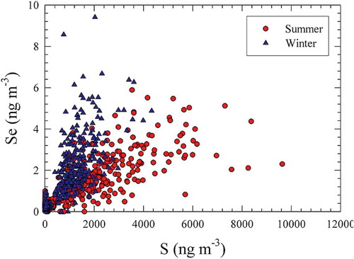
It is possible that there is sufficient atmospheric processing of the emissions that they produce data such as shown in Figure 2. These data were produced by the analysis of samples collected in Underhill, VT (Polissar et al., 2001a). Two edges can be observed in this figure: one for winter points and one for summer points. Both the Se and the SO₂ that is the precursor for the observed particulate S are emitted primarily from coal-fired power plants. However, differences in the rates of conversion of S(IV) to S(VI) between summer and winter require two factors to fully reproduce the observed concentrations and the sum of their contributions being assigned as the coal-fired power plant contributions to the measured PM_2.5 mass.

Figure 2. Plot of Se and S measured in PM_2.5 samples collected in Underhill, VT.

Multivariate methods

Target transformation factor analysis

In the late 1970s, target transformation factor analysis (Hopke, 1988) was developed to avoid the problems associated with principal component analysis (PCA) and other forms of factor analysis that center the data before performing the analyses. PCA was rapid given the computational power available, but only provided qualitative information about the nature of the source profile compositions and the relative importance of a given source to the observed concentrations. It did not provide a quantitative apportionment similar to that of a CMB analysis. However, TTFA was capable of providing such a resolution. It was initially applied to a number of data sets collected during the Regional Air Pollution Study (RAPS) of the ambient aerosol in St. Louis, MO, in the period of 1975 to 1977 and was used for a limited number of studies. As new methods became available, this approach has become obsolete.

Unmix

Henry and coworkers (Henry and Kim, 1989; Kim and Henry, 1999, 2000) have developed alternative methods based on eigenvector methods. The initial model was SAFER, a geometrical approach to fitting nonnegative source compositions and contributions, and has evolved into Unmix (EPA, 2007). It is based on an eigenvector decomposition of the ambient data as the basis for defining the feasible region of the solution and defining the edges (Henry, 2003). However, eigenvector decompositions are not appropriate for heteroskedastic data (Paatero and Tapper, 1993). It assumes that the edges that are found represent the source profiles. The uncertainties are then estimated based on a bootstrapping approach (Effron and Tibshirani, 1993). However, the edges are only the true source profile if there are really zero source contribution samples in the data set. For many sources, it is unlikely that the contribution goes to zero or sufficiently low that it can be assumed to be zero. For example, motor vehicle traffic rarely disappears entirely. Similarly, long-range-transported sulfate particles in the eastern United States are rarely going to have low or zero values. They will have minimum values, but that means that the edge is offset from its true value and the contributions will not be accurately estimated. This problem is termed rotational ambiguity (Paatero et al., 2002; Paatero and Hopke, 2009). This problem is assumed to be solved by Unmix, and thus, some of the uncertainties estimated by Unmix are likely to be underestimated.

Unmix has been applied to a number of air quality data sets, including airborne PM (Chen et al., 2002; Lewis et al., 2003; Hu et al., 2006; Li et al., 2010; Pancras et al., 2013), particle number size distribution (Kim et al., 2004), and semivolatile compounds associated with airborne PM (Miller et al., 2002; Hellén et al., 2003; Mukerjee et al., 2008; Song et al.; 2008, Li et al., 2011; Khairy and Lohmann, 2013; Patoskoski et al., 2014). Until the most recent version (V6), there were limitations to the number of factors that could be extracted, and it often could not find a feasible solution. Thus, it has experienced only limited applications.

As an example, Patokoski et al. (2014) applied Unmix to VOC measurements made in Helsinki and Hyytiälä, Finland. The VOCs were measured with proton transfer reaction mass spectrometry (PTR-MS), yielding data for methanol (M33), acetaldehyde (M45), acetone (M59), isoprene, methylbutenol (MBO) fragments and furan (M69), methylvinylketone (MVK) or methacrolein (M71), methyl ethyl ketone (MEK) (M73), benzene (M79), methylbutenol (M87) toluene (M93), hexenal (M99), hexanal and cis-3-hexenol (M101), and monoterpenes (M137). In Hyytiälä, the measured trace gases (NOx, CO, O₃) and aerosol particle number concentrations were also included in the analysis. Traffic and distant sources were identified at both sites. The distant source was characterized by more oxygenated compounds. In Helsinki, additional single-species sources of methanol and acetone were found in winter and two biogenic sources were identified in spring. At the rural site in Hyytiälä, there were also regional, accumulation-mode-particle, and monoterpene sources. At both sites, the anthropogenic sources contributed more in winter when the mixing heights were reduced and dilution was less. In addition to the diurnal cycles of VOCs, the biogenic activity was evident also in the source estimates in spring at both sites. Furthermore, the regional VOC sources were present continuously at Hyytiälä.

Positive matrix factorization

Positive matrix factorization (PMF) was developed by Paatero (Paatero and Tapper, 1993, 1994; Paatero, 1997a) and has become the most widely used source resolution method following its release by the U.S. EPA (EPA, 2014b). The concept in this method is to utilize an explicit least-squares formulation of the mass balance problem presented in eq 1. The eigenvector approaches used in TTFA and Unmix represent an implicit unweighted least-squares fit to the data (Malinowski, 2002). Since environmental data do not possess uniform uncertainties, the regression problem should not be solved without proper weighting, but an eigenvector approach only permits scaling by a row or a column. Data points cannot be individually weighted (Paatero and Tapper, 1993). PMF solves the receptor modeling problem by minimizing a weighted objective function given by

(4)

where s_ij is an estimate of the uncertainty for the jth species in the ith sample. This uncertainty is a combination of measurement error and the variability in the source profile value. As discussed earlier, there is natural variability in the source profile values, given that it is not a fundamental property of the activity in the same way that a spectrum is a fundamental property of a chemical compound.

PMF has been implemented in two algorithms. Initially, PMF2 was developed (Paatero, 1997a) to provide rapid solution to the model presented in eq 1. PMF2 was initially applied to data sets of major ion compositions of daily precipitation samples collected over a number of sites in Finland (Juntto and Paatero, 1994) and samples of bulk precipitation (Anttila et al., 1995) in which they are able to obtain considerable information on the sources of these ions. Polissar et al. (1996) applied the PMF2 program to Arctic data from seven National Park Service sites

in Alaska as a method to resolve the major source contributions more quantitatively. Polissar et al. (1998b) reanalyzed the Alaska data and proposed an approach to uncertainty estimation that has now been widely used in PMF applications. It should be noted that the rules of thumb provided to estimate the uncertainties were derived by extensive testing to find an approach that provided useful results. It has no statistical basis, and other approaches to error estimation may provide superior results.

In the late 1990s, a need was identified to be able to solve more complex problems because not all mass balance problems are represented by the bilinear model in eq 1. For example, data obtained from a series of samples collected with a cascade impactor as a function of time are a three-way data tensor (size, composition, time). Information is lost if the data are combined to produce a matrix for analysis. Thus, a more flexible solver was needed, and Paatero (1999) developed the multilinear engine that can solve any problem that can be expressed as a sum of product terms.

These two algorithms have a number of differences in how the solutions are obtained. One of the most important is the approaches to applying nonnegativity constraints (Kim and Hopke, 2007). In PMF2, the objective function in eq 4 is augmented with “penalty” functions that increase as the solution values approach zero (Paatero, 1997a). Alternatively, EPA PMF uses traditional nonnegative least-squares constraints similar to those described in Lawson and Hanson (1974) and Wang and Hopke (1989). Therefore, the PMF2 nonnegativity constraints force solutions toward the center of the feasible region of the solution and away from the boundaries where factor values would approach zero. However, the EPA PMF approach would permit any factor value as long as it is nonnegative, and the solution space will be searched closer to the periphery of the feasible region.

PMF has now become the most widely used receptor model, with more than 1000 papers reporting its application. It has been applied to apportionment of airborne particulate matter (e.g., Polissar et al., 1996; Polissar et al., 1998; Lee et al., 1999; Lee and Hopke, 2006; Lee et al., 2006; VanCuren and Gustin, 2015), precipitation (e.g., Juntto and Paatero, 1994; Anttila et al., 1995; Tiwari et al., 2015), VOCs (Zhao et al., 2004; Kim et al., 2005), and Aerosol Mass Spectrometry (Lanz et al., 2007; Aiken et al., 2008; Ulbrich et al., 2009; Zhang et al., 2011) data with a sharp rise in its use after the release of the EPA version of PMF (EPA, 2014b).

The most recent release of EPA PMF (V5.0) incorporates substantially improved error estimation methods (Paatero et al., 2014) that attempt to estimate the errors arising from the inherent uncertainties in the measured data as well as the rotational ambiguity in the solution. Brown et al. (2015) describe these methods and their application to presenting PMF solutions for various kinds of environmental data.

Constrained models

As mentioned earlier, adding constraints to the least-square fitting process can reduce the extent of rotational ambiguity. With PMF being applied through the use of the multilinear engine (Paatero, 1999), it is possible to build constraints into the model, as was done in two studies where there was an effort to separate multiple sources of similar composition (Amato et al., 2009a; Escrig et al., 2009). Amato et al. (2009a) applied the multilinear engine to data from an urban background site in Barcelona, Spain, to quantify the contribution of road dust resuspension to PM₁₀ and PM_2.5 concentrations. A recent emission profile of local resuspended road dust had been previously obtained (Amato et al., 2009b). This a priori information was introduced into the model as auxiliary terms in the object function to be minimized by the implementation of so-called “pulling equations” (Paatero and Hopke, 2009).

Escrig et al. (2009) applied a similar approach to speciated PM10 data obtained at three air quality monitoring sites between 2002 and 2007 in a highly industrialized area in Spain. The source apportionment of PM in this area is an especially difficult task. There are industrial mineral dust emissions that needed to be separately quantified from the natural sources of mineral PM. On the other hand, the diversity of industrial processes in the area results in a puzzling industrial emissions scenario. The availability of specific source profiles for particular major industrial emissions permitted the resolution of the industrial emissions from other sources, providing an opportunity to quantitatively evaluate the effectiveness of abatement programs for regional air quality improvement.

Amato and Hopke (2012) have applied constraints to combine the analysis of the three sites in the St. Louis, MO, area into a single analysis such that known source profiles could be worked into the analysis. To obtain good target profiles for major sources derived from data independent from the particle composition data collected at each of the three sites, additional high-time-resolution data collected as part of the St. Louis–Midwest Supersite study was employed. Applying PMF to these data permitted extraction of profiles for the copper products plant, the zinc smelter, and the steel mill factor. Average tailpipe emissions profiles were taken from Schauer et al. (2006). These profiles were taken as targets and introduced in the ME continuation run with the aim of extending the number of sources found. The results were substantially improved over the original results (Lee et al., 2006; Lee and Hopke, 2006).

Constraints have shown to be of sufficient value that they have now been incorporated into the EPA version of PMF in version 5.0.14 (EPA, 2014b). Using them requires a multiple step analysis in which an initial solution is obtained and then constraints applied to the continuation run. Details of how to perform such analyses are provided in the user’s manual (EPA, 2014c). Sofowote et al. (2015a) described how to construct constraints using available data. They analyzed data from five sites across Ontario, Canada, assuming that all of the sites would be affected by the same distant sources via long-range transport. Eight factors were found to be common across these sites. These factors had profiles that varied greatly from one site to the other, suggesting that the PMF solutions were impacted by some rotational ambiguity. The features in the EPA PMF V5 were used to impose mathematical constraints that guided the factor solutions. These constraints reduce the rotational space. In situations where major emissions sources are known and located in the neighborhood of receptors, or emissions inventories and literature source profiles exist, it is easy to use these profiles to force the factor solutions to conform to the expected signatures. In this case, reported source profiles were neither available nor applicable due to the large spatial span of potential sources and receptor sites. This work described how such constraints can be generated and used in these complex situations. The constrained solution was then applied to provide the source apportionments for the PM2.5 at each site (Sofowote et al., 2015b). Thus, there are now tools available where a priori information can be used in EPA PMF to fit known sources and then be able to derive the remaining source profiles to appropriately fit the data.

Other complex models

An advantage of the explicit least-squares formulations such as PMF is that conceptual models can be built and tested based on the nature of the processes underlying the creation of the data set. A number of such models have been developed to maximize the information recovery from the collected data sets.

Multiple sample type data

In many panel studies of the effects of airborne particles on health, measurements are made in multiple environments. For example, Hopke et al. (2003) report on the analysis of elderly subjects living in a single multifamily residence. Measurements were made at a central outdoor site, an unoccupied room in the building, and using personal samplers on specific individuals. Thus, different sources will affect different sample types. Only “external” sources of ambient particles will affect the outdoor samples. However, ambient particles will penetrate into indoor air and add to the exposure observed in the indoor and personal samples. Indoor sources such as cooking and the use of personal care products will not affect the outdoor samples. The expanded receptor model for this study can be expressed as

(5)

(6)

where i is the individual (subject or participant) index, j is the species index, d is the sampling date index, t is the type index, N is the number of external sources, H is the number of internal sources, x_ijdt denotes the concentration of species j in the sample of type t collected by subject i on date d, g_ipdt denotes the contribution of source p to the sample of type t collected by subject i on date d, and f_jp denotes the relative concentration of species j in source p.

This model has been used to analyze data for cardiac patients in the Raleigh–Chapel Hill area of North Carolina (Zhao et al., 2006) and to analyze data for asthmatic children attending a special school for moderate to severe asthmatics in Denver, CO (Zhao et al., 2007a). In the case of the Denver study, four external sources and three internal sources were resolved from the PM_2.5 data for the three different environments. Secondary nitrate and motor vehicle emissions were the two largest external sources in this study. Cooking was the largest internal source. A significant influence of indoor tobacco smoking on daily personal exposures to particles was observed for those houses in which smokers reside and the environmental tobacco smoke contribution correlated with urinary cotinine levels in these urban schoolchildren. The influence of the high traffic flow outside the school on the indoor air quality was also observed.

Time synchronization model

One of the major developments in atmospheric monitoring over the past 15 years has been the deployment of more real-time and near-real-time instruments. However, these instruments collect data at different frequencies ranging from a few minutes to a few hours. Higher frequency data have the advantage that transient events can be observed that can often provide edge points that would otherwise be averaged out of a longer interval sample (Lioy et al., 1989). Thus, it is not desirable to average the higher frequency data to the longer time interval instrument data in the suite of data. There is no way to split the longer integration time data down to the shorter time intervals, so it is necessary to have models that permit each set of data to be included within its own measurement frequency. Such models have been applied to several of the sets of data from the EPA Supersite program. Zhou et al. (2004a) analyzed data from Pittsburgh, PA, while Ogulei et al. (2005) used the same model for data from Baltimore, MD. The model has been examined further using simulated data (Liao et al., 2013) and it was found that the model performed well. It has also been applied to provide VOC and PM_2.5 source apportionments that then were used to apportion risk in the exposed populations (Liao et al., 2015).

Multiway data

The vast majority of applications of PMF are to matrices that provide information on chemical properties of a series of samples. However, there is also the potential for data with increased dimensionality. For example, if particles are segregated by aerodynamic diameter into multiple samples collected during a given time interval that are then analyzed for their chemical composition, the data set is then a three-way array or tensor consisting of size, composition, and time period. Data for a single variable like PM_2.5 mass concentrations could be collected from multiple sites across an area so that the three ways would be latitude, longitude, and concentration. If those samples were then analyzed for composition, there would then be a four-way array. Various such applications of PMF have been made and demonstrate how conceptual models can be built to fit the data, rather than all data being fitted to the same bilinear model.

Spatially distributed data

Paatero et al. (2003) examined a spatial data set of PM_2.5 mass concentrations measured every third day at more than 300 locations in the eastern United States during 2000. The basic PMF model was enhanced by modeling the dependence of PM_2.5 concentrations on temperature, humidity, pressure, ozone concentrations, and wind velocity vectors. The model comprises 12 general factors, augmented by 5 urban-only factors intended to represent excess concentration present in urban locations only. The flux density maps showed the major transport patterns of PM_2.5. For example, they show the increase in particle mass as the air moves from the regions of the gaseous precursor (SO₂), and the SO₂ is converted into sulfate. Recognition of this combination of transport and transformation is necessary in order that control procedures can be targeted to significant causes of high PM_2.5 concentrations.

A different spatial model was developed by Chuienta et al. (2004) for the analysis of the spatial patterns and possible sources affecting haze and its visual effects in the southwestern United States. The data are from the Measurement of Haze and Visual Effects (MOHAVE) project and were collected during the late winter and midsummer of 1992 at the monitoring sites in four states (i.e., California, Arizona, Nevada, and Utah). The resulting three-way data array was analyzed by a four-product-term model. This study makes a direct effort to include wind patterns as a component in the model in order to obtain the information of the spatial patterns of source contributions. The solution is computed using the conjugate gradient algorithm with applied nonnegativity constraints. For the winter data set, reasonable solutions contained six sources and six wind patterns. The analysis of summer data required seven sources and seven wind patterns.

Size–composition–time data

There are a number of devices that can separate particles by size such that samples can be collected that represent a relatively limited particle size range. The most common of these systems is a cascade impactor, in which particles are sequentially separated and collected for analysis. Most of these systems are manually operated, so there is considerable effort involved in collecting a series of samples. However, there have been several systems developed for collecting a time series of time- and size-resolved samples that can then be analyzed. One of these systems is the rotating DRUM impactor sampler (Raabe et al., 1988) that collects the particles on Mylar films placed on a rotating drum under the nozzle that determines the aerodynamic behavior of the particles. The resulting samples can be analyzed using synchrotron XRF (Knochel, 1989) to provide the three-way data set.

Different sources have different size-composition profiles in their emissions (Dodd et al., 1991). Thus, a source profile for size segregated data is a matrix of composition as a function of size, and therefore, a special model is required to properly account for the processes by which the particles are formed and emitted into the atmosphere. The main equation of the model is as follows:

(7)

where is the three-way array of observed data, ⊗ represents a Kroneker product (Burdick, 1995; Kiers, 2000) of the source profile array with the contribution matrix, A(I,P), P is the number of factors, and is the three-way array of residuals.

This model has been applied to several data sets, including three-stage DRUM impactor data from Detroit, MI, with the samples collected between February and April 2002 (Pere-Trepat et al., 2007), and eight-stage DRUM impactor data from the Washington–Dulles International Airport (Li et al., 2013). For the Detroit data (Pere-Trepat et al., 2007), nine factors were identified: road salt, industrial (Fe + Zn), cloud-processed sulfate, two types of metal works, road dust, local sulfate source, sulfur with dust, and homogeneously formed sulfate. Road salt had high concentrations of Na and Cl. Mixed industrial emissions are characterized by Fe and Zn. The cloud-processed sulfate had a high concentration of S in the intermediate size mode. The first metal works was represented by Fe in all three size modes and by Zn, Ti, Cu, and Mn. The second included a high concentration of small-size particle sulfur with intermediate-size Fe, Zn, Al, Si, and Ca. Road dust contained Na, Al, Si, S, K, and Fe in the large size mode. The local and homogeneous sulfate factors show high concentrations of S in the smallest size mode, but different time-series behavior in their contributions. Sulfur with dust is characterized by S and a mix of Na, Mg, Al, Si, K, Ca, Ti, and Fe from the medium and large size modes. The analysis utilized light absorption measurements at 4 wavelengths, 350, 450, 550, and 650 nm, to provide limited information on the carbonaceous components in the samples.

At Dulles International Airport, five major emission sources—soil, road salt, aircraft landings, transported secondary sulfate, and local sulfate/construction—were identified (Li et al., 2013). Aircraft landing was notable, for it had not previously been identified as a significant source of PM_2.5. Its pattern showed small particles of sulfur, zinc, bromine, zirconium, and molybdenum. This factor is assigned to particles that are emitted during landings. The sulfur and zinc come from tire wear. These elements are key constituents in tires. Often a visible puff of smoke is observed at touchdown. There is considerable frictional heat produced at this instant and particles are generated across the particle size range. Both zirconium and molybdenum are used in high-temperature greases such as might be used to lubricate bearings that would undergo significant heat stress. The energy deposited in the bearings can be expected to liberate particles from the lubricants. The study showed that time- and size-resolved DRUM data can assist in the identification of the airport emission sources and atmospheric processes leading to the observed ambient concentrations.

Ensemble methods

It is possible to integrate the results of chemical transport models with receptor models. These approaches have been termed ensemble methods. Lee et al. (2009) first introduced this approach in which multiple receptor modeling approaches were used for PM apportionment in conjunction with a short-term application of CMAQ for Atlanta, GA. A normal CMB, one using molecular markers, and the Lipschitz global optimizer (LGO) approach with gaseous data were used to obtain three sets of apportionments. A PMF analysis was also performed on daily 24-hr integrated sample composition data from the Jefferson Street site in Atlanta. CMAQ results were available for several limited time periods (July 2001 and January 2002). Nine pollutant sources were identified. Weighted-average source contributions were obtained for each source on each day from the multiple receptor and CTM solutions. These source contributions were then combined with the ambient data in a CMB–LGO analysis to obtain a new set of ensemble-based source profiles. These profiles were then applied to the ambient data in a final CMB–LGO analysis to obtain their final source apportionments. They felt that the resulting apportionment better reflected the likely source contributions than any of the individual method results. Balachandran et al. (2012) further analyzed these results and provided a method uncertainty analysis. Maier et al. (2013) applied the approach to East St. Louis, IL, based on the results of the analysis of daily PM_2.5 samples collected at the St. Louis–Midwest Supersite.

Balachandran et al. (2013) then extended the approach by using a Bayesian ensemble average of the multiple source apportionments to produce source profile distributions. Source profiles sampled from these distributions were then used in a final CMB analysis to produce the final results. They report that the results of this approach provide a better representation of some sources particularly biomass burning because of improved correlations of the source contributions with the traditional markers of biomass combustion (levoglucosan and potassium).

Methods using local wind data

Conditional probability function (CPF)

To analyze point-source impacts from various wind directions, the conditional probability function (CPF) (Kim et al., 2003) was calculated using source contribution estimates coupled with wind direction values measured on site. To minimize the effect of atmospheric dilution, daily fractional mass contribution from each source relative to the total of all sources was used, rather than using the absolute source contributions. The same daily fractional contribution was assigned to each 3-hr period of a given day to match to the 3-hr average wind direction. Specifically, the CPF is defined as

(8)

where m_Δθ is the number of occurrences from wind sector Δθ that exceeded the threshold criterion, and n_Δθ is the total number of data from the same wind sector. The threshold is set to a relatively high percentile value in the distribution of fractional contributions from a given source. The sources are likely to be located to the directions that have high conditional probability values.

Nonparametric regression

Nonparametric regression (NPR) (Härdle, 1990) is a regression model without parameters since it estimates the expected value of concentration given wind direction. To find the directions of peaks in the ambient concentrations, Henry et al. (2002) suggested NPR using a Gaussian kernel as a nonsubjective alternative to the usual bar chart method that is highly dependent on the location and size of Δθ. NPR produces statistical confidence intervals as well as estimates of the location of peaks, and is able to separate closely located peaks. NPR was applied to the hourly measured cyclohexane data from two sites in Houston, TX. The triangulation of the peak directions estimated from two sites correctly pointed to the source (Henry et al., 2002; Yu et al., 2004; Kim and Hopke, 2004).

Nonparametric wind regression (NWR)

Henry et al. (2009) enhanced NPR by adding regression for wind speed as well as wind direction. For wind speed, the Epanechnikov kernel function is employed. It has been applied by Henry et al. (2009) to SO₂ data from East St. Louis, IL. Olson et al. (2011) applied nonparametric wind regression (NWR) to the concentrations of 13 organic source markers (10 polycyclic aromatic hydrocarbons and 3 hopanes) measured in time-integrated samples (24-hr and subdaily) collected near a highway in Las Vegas, NV. Cheng et al. (2014) applied NWR to estimate the impact of oil and natural gas exploration and production activities on local air quality in Pennsylvania’s Allegheny National Forest. They found effects on the local concentrations of NO_x and SO₂, as well as potential impacts on regional air quality.

Sustained wind incidence method

A further development was reported by Vedantham et al. (2012) in which the wind direction standard deviation is incorporated into the model, resulting in a reduction of the effect of data collected during highly unstable meteorological periods with large wind directional changes. Vedantham et al. (2012) applied the sustained wind incidence method (SWIM) to black carbon (BC) data to estimate the impact of the traffic due to expansion of a major highway in Las Vegas, NV. Data were collected both before and after the expanded lanes were open for use and the analysis showed a substantial increase in BC on the expanded highway section. Vette et al. (2013) also examined BC data, but in Detroit, MI, to apportion the BC contributions from various wind directions as part of a study looking at exposure of asthmatic children to diesel traffic.

Of these methods, CPF has been most widely used because it can be easily calculated using a spreadsheet while the other approaches require access to a program to do the fitting. Although some of the papers indicate the availability of the software that implements the nonparametric methods, the programs are not generally available.

Methods incorporating back trajectories

The dispersion models describe the transport of the particles from a source to the sampling location. However, using an analogous model of atmospheric transport, it is possible to calculate the position of the air being sampled backward in time from the receptor site from various starting times throughout the sampling interval. The trajectories are then used in residence time analysis (RTA), areas of influence analysis (AIA), quantitative bias trajectory analysis (QTBA), potential source contribution function (PSCF), and residence time weighted concentrations (RTWC). AIA, QTBA, and RTWC have only been used in a single publication for each method, and those results are reviewed by Seigneur et al. (1997). PSCF and simplified QTBA have been primarily used in recent published studies.

Potential source contribution function (PSCF)

The potential source contribution function (PSCF) receptor model was originally developed by Ashbaugh et al. (1985). It has been applied in a series of studies over a variety of geographical scales (Cheng et al., 1993a, 1993b; Gao et al., 1993, 1994, 1996). Air parcel back trajectories ending at a receptor site are represented by segment endpoints. Each endpoint has two coordinates (e.g. latitude, longitude) representing the central location of an air parcel at a particular time. To calculate the PSCF, the whole geographic region covered by the trajectories is divided into an array of grid cells whose size is dependent on the geographical scale of the problem so that the PSCF will be a function of locations as defined by the cell indices i and j.

Air parcel backward trajectories were related to the composition of collected material by matching the time of arrival of each trajectory at the receptor site. The movement of an air parcel is described as series of segment end points defined by their latitude and longitude. PSCF values for each grid cell were calculated by counting the trajectory segment endpoints that terminate within the grid cells. The number of endpoints that fall in the cell is . The number of endpoints for the same cell when the corresponding samples show concentrations higher than an arbitrarily criterion value is defined to be . The PSCF value for the cell is defined as

(9)

In the PSCF analysis, it is likely that the small values of n_ij produce high PSCF values with high uncertainties. In order to minimize this artifact, an empirical weight function W (n_ij) proposed by Zeng and Hopke (1989) is commonly applied when the number of the endpoints for a particular cell was less than about three times the average values of the endpoints per cell.

Although the trajectory segment endpoints are subject to uncertainty, a sufficient number of endpoints should provide accurate estimates of the source locations if the location errors are random and not systematic. Cells containing emission sources would be identified with conditional probabilities close to 1 if trajectories that have crossed the cells effectively transport the emitted contaminant to the receptor site. The PSCF model thus provides a means to map the source potentials of geographical areas. It does not apportion the contribution of the identified source area to the measured receptor data.

Xie et al. (1999) used PSCF to examine the locations of the sources identified by the PMF analysis of the data from Alert. The results of these analyses were in agreement with earlier efforts that examined the PSCF maps for the individual chemical constituents in the particle samples. Poissant (1999) used PSCF to examine the likely source locations for total gaseous mercury observed in the St Lawrence River valley. During the winter, fall, and spring period the distribution of potential sources reasonably reproduces the North American Hg emission inventory. However, because a single fixed criterion was over the entire year and transport from many of the strong source areas was weak during the summer months, few source areas were observed during the summer data where the concentrations were the lowest. Polissar et al. (2001b) examined the particle data (black carbon, light scattering, and condensation nuclei counts) collected at Point Barrow, AK. They found that they could distinguish between biogenic sources of the small particles seen only with the condensation nuclei counter and anthropogenic larger particles that scatter and absorb light. The biogenic particles came primarily from the open areas of the North Pacific Ocean, whereas most of the anthropogenic particles came from known industrialized areas of Russia.

PSCF has been evaluated in the same applications involving large-scale wildfires where the origin of the smoke particles was well known. Cheng and Lin (2001) examined smoke from a large fire in Central America. Begum et al. (2005) used the transport of a fire plume from Quebec, Canada, to Philadelphia, PA, to test the approach. In both cases, there was excellent agreement between the identified areas of high probably and the actual locations of the fires.

Software to prepare PSCF maps are now readily available. TrajStat (Wang et al., 2009) is available at http://www.meteothinker.com/products/trajstat_features.html. Another implementation is in MetCor and is described in Sofowote et al. (2010a, 2010b) (http://www.chemistry.mcmaster.ca/faculty/mccarry/MC_downloads.html).

Simplified quantitative trajectory bias analysis (SQTBA)

Quantitative trajectory bias analysis (QTBA) was developed by Keeler (1987) as a multiple-site approach to be able to better identify source regions for measured downwind high concentrations. It was applied to data collected at a number of sites in the northeastern United States (Keeler and Samson, 1989). However, it is very difficult to implement, and thus, the full approach has not been applied elsewhere. It is possible to use the basic framework but simplify the analysis such that it becomes a practical approach to apply (Zhou et al., 2004b; Brook et al., 2004).

The probability of a tracer arriving at a point (x, y) at time t is given as

(10)

where Q(x, y, t|x^’, y,^’, t^’) is the transition probability density function of an air parcel located at (x^’, y^’) and time t^’ arriving at the receptor site (x, y) at time t.

The transition probability Q is assumed to be approximately normally distributed about the trajectory with a standard deviation that increases linearly with time upwind:

(11)

where (X, Y) is the coordinate of the grid center and x^’(t^’) and y,^’(t ^’) are the coordinates of the center line of the trajectory. The σ_x and σ_y are approximated by

(12)

with a dispersion speed, a, equal to 5.4 km/hr (Samson, 1980). The potential mass-transfer field for a given trajectory, , was integrated over the upwind period, τ, of each trajectory to produce a two-dimensional probability of natural transport field.

` (13)

The resulting natural transport potential field, , for trajectory k, was weighted by the corresponding concentration, χ_k(x,y), yielding a concentration-weighted mass transfer potential field:

(14)

This definition of the weighted potential field is different from the definition given in Keeler (1987) since it is not divided by the sum of concentrations. Thus, the weighted potential field in eq (17) has the dimension of concentrations.

In PSCF, when cells are crossed by small number of trajectories, false source areas may be found if some of the trajectories also pass real source areas. This problem was solved by Cheng et al. (1993a, 1993b) by down-weighting the PSCF values. This “tailing effect” (Cheng and Lin, 2001) problem also exists for SQTBA and RTWC. To solve this problem, the SQTBA field was down-weighted empirically by the following method.

A coefficient c_r is defined:

(15)

where K is total number of trajectories and t₀ is the length of the longest trajectory. The final SQTBA field is obtained by dividing the concentration-weighted field by unweighted field:

(16)

The weighted field has the dimensions of concentrations and the unweighted natural field is dimensionless so the final SQTBA field has the dimensions of concentrations. This approach has been used in several studies (Zhou et al., 2004b; Brook et al., 2004; Zhao et al., 2007b).

Future directions

We now have fairly sophisticated data analysis tools like PMF with good uncertainty estimation methods. These methods have been made readily available to the atmospheric community. We have a suite of methods to utilize external information, such as local meteorology and longer range Lagrangian trajectories. Thus, what new methods can be anticipated in the future?

There is increasing interest in Bayesian methods and there has been some initial work in this direction (e.g., Park et al., 2014; Hackstadt and Peng, 2014). However, the conceptual framework and the statistical computations are more complex so that it is difficult for investigators to get started using this approach. In addition, there remain considerable questions about how the prior distributions are developed and the sensitivity of the resulting apportionments to those priors. Do the priors adequately address both the measurement uncertainties in the ambient data and the variability in the source profiles? Additional work is required to better understand the place of Bayesian approaches in receptor modeling.

As has been shown by a number of studies using high-time-resolution data (e.g., Ogulei et al., 2005, Sofowote et al., 2013), it is possible to obtain improved resolution of sources by obtaining more edge points because of the separation of sources driven by changing wind directions and differences in operating schedules. Semicontinuous sampling systems like the rotating drum impactor also provide time-resolved data that can be combined with semicontinuous in situ instruments such as an aethalometer and/or a field organic/elemental carbon analyzer to open additional opportunities for improved source identification and separation. More extensive data on time resolved organic compounds will also become more readily available. Thus, we can anticipate larger, richer data sets that will permit better resolution of the sources and hence increased accuracy in the resulting contributions that can then better inform the development of air quality control strategies.

Conclusions

There are now a number of mature mathematical data analysis methods that can be applied to concentration data to estimate source apportionments. The methods are generally available in relatively easy-to-use formats, and that has led to a rapid expansion of their application to a variety of data types. There are now capabilities of combining data from multiple sites or building specific conceptual data models that can be fitted to specific types of available data. There are thus greatly improved tools available for use, and their application to specific air quality problems should help to provide additional insights into the source/receptor relationships that can then guide the development of more effective air quality management strategies.

Acknowledgments

The author acknowledges all of the people over the years who have seen the opportunity to develop and apply better data analysis tools to atmospheric data. They also need to acknowledge the improved data they have to analyze because of the development and deployment of improved measurement technologies that provide better time and species resolution.

ORCID

Philip K. Hopke

http://orcid.org/0000-0003-2367-9661

Additional information

Notes on contributors

Philip K. Hopke

Philip K. Hopke is a professor in the Department of Chemical and Biomolecular Engineering and the Institute for a Sustainable Environment at Clarkson University. He is also the director of Clarkson’s Center for Air Resources Engineering and Science and a managing partner of Consulting for Health, Air, Nature, & a Greener Environment, LLC.

References

- Aiken, A.C., P.F. DeCarlo, J.H. Kroll, D.R. Worsnop, J.A. Huffman, K. Docherty, I.M. Ulbrich, C. Mohr, J.R. Kimmel, D. Sueper, Q. Zhang, Y. Sun, A. Trimborn, M. Northway, P.J. Ziemann, M.R. Canagaratna, T.B. Onasch, R. Alfarra, A.S.H. Prévôt, J. Dommen, J. Duplissy, A. Metzger, U. Baltensperger, and J.L. Jimenez. 2008. O/C and OM/OC ratios of primary, secondary, and ambient organic aerosols with high resolution time-of-flight aerosol mass spectrometry. Environ. Sci. Technol. 42:4478–85. doi:10.1021/es703009q
- Amato, F., M. Pandolfi, A. Escrig, X. Querol, A. Alastuey, J. Pey, N. Perez, and P.K. Hopke. 2009a. Quantifying road dust resuspension in urban environment by multilinear engine: A comparison with PMF2. Atmos. Environ. 43:2770–80. doi:10.1016/j.atmosenv.2009.02.039
- Amato, F., M. Pandolfi, M. Viana, X. Querol, A. Alastuey, and T. Moreno. 2009. Spatial and chemical patterns of PM10 in road dust deposited in urban environment. Atmos. Environ. 43:1650–59. doi:10.1016/j.atmosenv.2008.12.009
- Anderson, T.W. 1984. An Introduction to Multivariate Statistical Analysis (2nd ed.). New York, NY: Wiley.
- Andriani, E., M. Caselli, G. de Gennaro, A. Giove, and C. Tortorella. 2011. Synergistic use of several receptor models (CMB, APCS and PMF) to interpret air quality data. Environmetrics 22:789–97. doi:10.1002/env.v22.6
- Anttila, P., P. Paatero, U. Tapper, and O. Jaarvinen. 1995. Application of positive matrix factorization to source apportionment: Results of a study of bulk deposition chemistry in Finland. Atmos. Environ. 29:1705–18. doi:10.1016/1352-2310(94)00367-T
- AQUELLA. 2007. “AQUELLA” Steiermark Bestimmung von Immissionsbeiträgen in Feinstaubproben Rep., Wien, Germany.
- Balachandran, S., J.E. Pachon, Y. Hu, D. Lee, J.A. Mulholland, and A.G. Russell. 2012. Ensemble-trained source apportionment of fine particulate matter and method uncertainty analysis. Atmos. Environ. 61:387–94. doi:10.1016/j.atmosenv.2012.07.031
- Balachandran, S., H.H. Chang, J.E. Pachon, H.A. Holmes, J.A. Mulholland, and A.G. Russell. 2013. Bayesian-based ensemble source apportionment of PM2.5. Environ. Sci. Technol. 47:13511–18. doi:10.1021/es4020647
- Begum, B.A., E. Kim, C.H. Jeong, D.W. Lee, and P.K. Hopke. 2005. Evaluation of the potential source contribution function using the 2002 Quebec forest fire episode. Atmos. Environ. 39:3719–24.
- Begum, B.A., S.K. Biswas, and P.K. Hopke. 2007. Source apportionment of air particulate matter by chemical mass balance (CMB) and comparison with positive matrix factorization (PMF) model. Aerosol and Air Qual. Res. 7:446–68.
- Belis, C.A., J. Cancelinha, M. Duane, V. Forcina, V. Pedroni, R. Passarella, G. Tanet, K. Douglas, A. Piazzalunga, E. Bolzacchini, G. Sangiorgi, M.G. Perrone, L. Ferrero, P. Fermo, and B.R. Larsen. 2011. Sources for PM air pollution in the Po Plain, Italy: I. Critical comparison of methods for estimating biomass burning contributions to benzo(a)pyrene. Atmos. Environ. 45:7266–75. doi:10.1016/j.atmosenv.2011.08.061
- Belis, C.A., F. Karagulian, B.R. Larsen, and P.K. Hopke. 2013. Critical review and meta analysis of ambient particulate matter source apportionment using receptor models in Europe. Atmos. Environ. 69:94–108. doi:10.1016/j.atmosenv.2012.11.009
- Bell, M.L., D.L. Davis, and T. Fletcher. 2004. A retrospective assessment of mortality from the London smog episode of 1952: The role of influenza and pollution. Environ. Health Perspect. 112:6–8. doi:10.1289/ehp.6539
- Blando, J.D., and B.J. Turpin. 2000. Secondary organic aerosol formation in cloud and fog droplets: A literature evaluation of plausibility, Atmos. Environ. 34:1623–32. doi:10.1016/S1352-2310(99)00392-1
- Blifford, I.H., and G.O. Meeker. 1967. A factor analysis model of large scale pollution. Atmos. Environ. 1:147–57. doi:10.1016/0004-6981(67)90042-X
- Brown, S.G., S. Eberly, P. Paatero, and G.A. Norris. 2015. Methods for estimating uncertainty in PMF solutions: Examples with ambient air and water quality data and guidance on reporting PMF results. Sci. Total Environ. 518:626–35. doi:10.1016/j.scitotenv.2015.01.022
- Brook, J.R., D. Johnson, and A. Mamedov. 2004. Determination of the source areas contributing to regionally high warm season PM2.5 in eastern North America. J. Air Waste Manage. Assoc. 54:1162–69. doi:10.1080/10473289.2004.10470984
- Burdick, D.S. 1995. An introduction to tensor products with applications to multiway data analysis. Chemom. Intell. Lab. Sys. 28:229–37. doi:10.1016/0169-7439(95)80060-M
- Cai, J., M. Zheng, C.-Q. Yan, H.Y. Fu, Y.J. Zhang, M. Li, Z. Zhou, and Y.-H. Zhang. 2015. Application and progress of single particle aerosol time-of-flight mass spectrometry in fine particulate matter research. Chin. J. Anal. Chem. 43:765–74. doi:10.1016/S1872-2040(15)60825-8
- Canagaratna, M.R., J.T. Jayne, J.L. Jimenez, J.D. Allan, M.R. Alfarra, Q. Zhang, T.B. Onasch, F. Drewnick, H. Coe, A. Middlebrook, A. Delia, L.R. Williams, A.M. Trim2007. born, M.J. Northway, P.F. DeCarlo, C.E. Kolb, P. Davidovits, and D.R. Worsnop. Chemical and microphysical characterization of ambient aerosols with the aerodyne aerosol mass spectrometer. Mass Spectrom. Rev. 26:185–222.doi:10.1002/mas.20115
- Caudill, M. 2012 Semi‐continuous metals monitoring in Ohio industrial communities. http://www.epa.gov/ttnamti1/files/2012conference/3BCaudill.pdf
- Chen, L.-W.A., B.G. Doddridge, R.R. Dickerson, J.C. Chow, and R.C. Henry. 2002. Origins of fine aerosol mass in the Baltimore–Washington corridor: Implications from observation, factor analysis, and ensemble air parcel back trajectories. Atmos. Environ. 36:4541–54.
- Cheng, M.-D., and C.-J. Lin. 2001. Receptor modeling for smoke of 1998 biomass burning in Central America. J. Geophys. Res. 106:22871–86. doi:10.1029/2001JD900024
- Cheng, M.D., P.K. Hopke, and Y. Zeng. 1993a. A receptor methodology for determining source regions of particle sulfate composition observed at Dorset, Ontario. J. Geophys. Res. 98:16839–49.
- Cheng, M-D., P.K. Hopke, L. Barrie, A. Rippe, M. Olson, and S. Landsberger. 1993b. Qualitative determination of source regions of long-range transported aerosol using data collected at Canadian High Arctic. Environ. Sci. Technol. 27:2063–71. doi:10.1021/es00047a011
- Chow, J.C., and J.G. Watson. 2002. Review of PM2.5 and PM10 apportionment for fossil fuel combustion and other sources by the chemical mass balance receptor model. Energy Fuels 16:222–60. doi:10.1021/ef0101715
- Chueinta, W., P.K. Hopke, and P. Paatero. 2004. Multilinear model for spatial pattern analysis of the measurement of haze and visual effects project. Environ. Sci. Technol. 38:544–54. doi:10.1021/es026356n
- Clarke, K., A.-C. Romain, N. Locoge, and N. Redon. 2012. Application of chemical mass balance methodology to identify the different sources responsible for the olfactory annoyance at a receptor-site. Chem. Eng. Trans. 30:79–84.
- Colucci, J.M., and C.R. Begeman. 1965. The automotive contribution to air-borne polynuclear aromatic hydrocarbons in Detroit. J. Air Pollut. Control Assoc. 15:113–22. doi:10.1080/00022470.1965.10468342
- Dodd, J.A., J.M. Ondov, G. Tuncel, T.G. Dzubay, and R.K. Stevens. 1991. Multimodal size spectra of submicrometer particles bearing various elements in rural air. Environ. Sci. Technol. 25:890–903. doi:10.1021/es00017a010
- El Haddad, I., N. Marchand, B. Temime-Roussel, H. Wortham, C. Piot, J.L. Besombes, C. Baduel, D. Voisin, A. Armengaud, and J.L. Jaffrezo. 2011. Insights into the secondary fraction of the organic aerosol in a Mediterranean urban area: Marseille. Atmos. Chem. Phys. 11:2059–2079. doi:10.5194/acp-11-2059-2011
- Efron, B., and R. Tibshirani. 1993. An Introduction to the Bootstrap. Boca Raton, FL: Chapman & Hall/CRC.
- El Haddad, I., N. Marchand, J. Dron, B. Temime-Roussel, E. Quivet, H. Wortham, J.L. Jaffrezo, C. Baduel, D. Voisin, J.L. Besombes, and G. Gille. 2009. Comprehensive primary particulate organic characterization of vehicular exhaust emissions in France. Atmos. Environ. 39:6190–98. doi:10.1016/j.atmosenv.2009.09.001
- El Haddad, I., N. Marchand, H. Wortham, C. Piot, J.-L. Besombes, J. Cosic, C. Chauvel, A. Armengaud, D. Robin, and J.-L. Jaffrezo. 2011. Primary sources of PM2.5 organic aerosol in an industrial Mediterranean city, Marseille. Atmos. Chem. Phys. 11:2039–58. doi:10.5194/acp-11-2039-2011
- Escrig Vidal, A., E. Monfort, I. Celades, X. Querol, F. Amato, M.C. Minguillón, and P.K. Hopke. 2009. Application of optimally scaled target factor analysis for assessing source contribution of ambient PM10. J. Air Waste Manage. Assoc. 59:1296–1307. doi:10.3155/1047-3289.59.11.1296
- Fine, P.M., G.R. Cass, and B.R.T. Simoneit. 2001. chemical characterization of fine particle emissions from fireplace combustion of woods grown in the northeastern United States. Environ. Sci. Technol. 35:2665–75. doi:10.1021/es001466k
- Fine, P.M., G.R. Cass, and B.R.T. Simoneit. 2004. Chemical characterization of fine particle emissions from the wood stove combustion of prevalent United States tree species. Environ. Eng. Sci. 21:705–21. doi:10.1089/ees.2004.21.705
- Friedlander, S.K. 1973. Chemical element balances and identification of air pollution sources. Environ. Sci. Technol. 7:235–40. doi:10.1021/es60075a005
- Friedlander, S.K. 1981. New developments in receptor modeling theory. In Atmospheric Aerosol Source/Air Quality Relationships, ed. E.S Macias and P.K. Hopke, 1–19. ACS Symposium Series 167. Washington, DC: ACS.
- Fuller, W.A. 1987. Measurement Error Models. New York, NY: J. Wiley & Sons.
- Gaarenstroom, P.D., S.P. Perone, and J.P. Moyers. 1977. Application of pattern recognition and factor analysis for characterization of atmospheric particulate composition in Southwest desert atmosphere. Environ. Sci. Technol. 11:795–800. doi:10.1021/es60131a003
- Gao, N., M.-D. Cheng, and P.K. Hopke. 1993. Potential source contribution function analysis and source apportionment of sulfur species measured at Rubidoux, CA during the Southern California Air Quality Study, 1987. Anal. Chim. Acta 277:369–80. doi:10.1016/0003-2670(93)80449-U
- Gao, N., M.D. Cheng, and P.K. Hopke. 1994. Receptor modeling for airborne ionic species collected in SCAQS, 1987. Atmos. Environ. 28:1447–70. doi:10.1016/1352-2310(94)90207-0
- Gao, N., P.K. Hopke, and N.W. Reid. 1996. Possible sources of some trace elements found in airborne particles and precipitation in Dorset, Ontario. J. Air Waste Manage. Assoc. 46:1035–47. doi:10.1080/10473289.1996.10467539
- George, C., M. Ammann, B. D’Anna, D.J. Donaldson, and S.A. Nizkorodov. 2015. Heterogeneous photochemistry in the atmosphere. Chem. Rev. 115:4218–58. doi:10.1021/cr500648z
- Gupta, A.K., K. Karar, and A. Srivastava. 2007. Chemical mass balance source apportionment of PM10 and TSP in residential and industrial sites of an urban region of Kolkata, India, J. Hazard. Mater. 142:279–87. doi:10.1016/j.jhazmat.2006.08.013
- Haagen-Smit, A.J. 1954. The control of air pollution in Los Angeles. Eng. Sci. 18:11–16.
- Hackstadt, A.J., and R.D. Peng. 2014. A Bayesian multivariate receptor model for estimating source contributions to particulate matter pollution using national databases. Environmetrics, 25:513–27. doi:10.1002/env.v25.7
- Härdle, W. 1990. Applied Nonparametric Regression. Cambridge, UK: Cambridge University Press.
- Hellén, H., H. Hakola, and T. Laurila. 2003. Determination of source contributions of NMHCs in Helsinki (60°N, 25°E) using chemical mass balance and the Unmix multivariate receptor models. Atmos. Environ. 37:1413–24. doi:10.1016/S1352-2310(02)01049-X
- Henry, R.C. 1991. Multivariate receptor models. In Receptor Modeling for Air Quality Management, ed. P.K. Hopke, 117–47. Amsterdam, The Netherlands: Elsevier.
- Henry, R.C. 1997. History and fundamentals of multivariate air quality receptor models. Chemomet. Intell. Lab. Syst. 37:37–42. doi:10.1016/S0169-7439(96)00048-2
- Henry, R.C. 2003. Multivariate receptor modeling by N-dimensional edge detection. Chemom. Intell. Lab. Syst. 65:179–89. doi:10.1016/S0169-7439(02)00108-9
- Henry, R.C., and B.-M. Kim. 1989. Extension of self-modeling curve resolution mixtures of more than three components. Part 1. Finding the basic feasible region. Chemomet. Intell. Lab. Syst. 8:205–16.
- Henry, R., G.A. Norris, R. Vedantham, and J.R. Turner. 2009. Source region identification using kernel smoothing. Environ. Sci. Technol. 43:4090–97. doi:10.1021/es8011723
- Hildemann, L.M., G.R. Cass, and G.R. Markowski. 1989. A dilution stack sampler for collection of organic aerosol emissions: Design, characterization and field tests. Aerosol Sci. Technol. 10:193–204. doi:10.1080/02786828908959234
- Hildemann, L.M., G.R. Cass, M.A. Mazurek, and B.R.T. Simoneit. 1993. Mathematical modeling of urban organic aerosol: Properties measured by high-resolution gas chromatography. Environ. Sci. Technol. 27:2045–55. doi:10.1021/es00047a009
- Hildemann, L.M., M.A. Mazurek, G.R. Cass, and B.R.T. Simoneit. 1994. Seasonal trends in Los Angeles ambient organic aerosol observed by high-resolution gas chromatography. Aerosol Sci. Technol. 20:303–17. doi:10.1080/02786829408959687
- Hildemann, L.M., W.F. Rogge, G.R. Cass, M.A. Mazurek, and B.R.T. Simoneit. 1996. Contribution of primary aerosol emissions from vegetation- derived sources to fine particle concentrations in Los Angeles. J. Geophys. Res. 101:19541–49. doi:10.1029/95JD02136
- Hopke, P.K. 1988. Target transformation factor analysis as an aerosol mass apportionment method: A review and sensitivity study. Atmos. Environ. 22:1777–92. doi:10.1016/0004-6981(88)90066-2
- Hopke, P.K. 2003. Recent developments in receptor modeling. J. Chemometrics 17:255–65. doi:10.1002/(ISSN)1099-128X
- Hopke, P.K. 2010. The application of receptor modeling to air quality data. Pollut. Atmos. September:91–109.
- Hopke, P.K. 2015. Applying multivariate curve resolution to source apportionment of the atmospheric aerosol. In 40 Years of Chemometrics, ed. B.K. Lavine, 129–157. Symposium Series. Washington, DC: American Chemical Society.
- Hopke, P.K., E.S. Gladney, G.E. Gordon, W.H. Zoller, and A.G. Jones. 1976. The use of multivariate analysis to identify sources of selected elements in the Boston urban aerosol. Atmos. Environ. 10:1015–25. doi:10.1016/0004-6981(76)90211-0
- Hopke, P.K., R.E. Lamb, and D.F.S. Natusch. 1980. Multielemental characterization of urban street dust. Environ. Sci. Technol. 14:164–72. doi:10.1021/es60162a006
- Hopke, P.K., Z. Ramadan, P. Paatero, G. Norris, M. Landis, R. Williams, and C.W. Lewis. 2003. Receptor modeling of ambient and personal exposure samples: 1998 Baltimore Particulate Matter Epidemiology-Exposure Study. Atmos. Environ. 37:3289–302. doi:10.1016/S1352-2310(03)00331-5
- Hu, S.H., R. McDonald, D. Martuzevicius, P. Biswas, S.A. Grinshpun, A. Kelley, T. Reponen, J. Lockey, and G. LeMasters. 2006. UNMIX modeling of ambient PM2.5 near an interstate highway in Cincinnati, OH, USA. Atmos. Environ. 40:S378–95. doi:10.1016/j.atmosenv.2006.02.038
- Isaacman, G., N.M. Kreisberg, L.D. Yee, D.R. Worton, A.W.H. Chan, J.A. Moss, S.V. Hering, and A.H. Goldstein. 2014. Online derivatization for hourly measurements of gas- and particle-phase semi-volatile oxygenated organic compounds by thermal desorption aerosol gas chromatography (SV-TAG). Atmos. Meas. Technol. 7:4417–29. doi:10.5194/amt-7-4417-2014
- Junninen, H., J. Mønster, M. Rey, J. Cancelinha, K. Douglas, M. Duane, V. Forcina, A. Müller, F. Lagler, L. Marelli, A. Borowiak, J. Niedzialek, B. Paradiz, D. Mira-Salama, J. Jimenez, U. Hansen, C. Astorga, K. Stanczyk, M. Viana, X. Querol, R.M. Duvall, G.A. Norris, S. Tsakovski, P. Wåhlin, J. Horak, and B.R. Larsen. 2009. Quantifying the impact of residential heating on the urban air quality in a typical European coal combustion region. Environ. Sci. Technol. 43:7964–70. doi:10.1021/es8032082
- Juntto, S., and P. Paatero. 1994. Analysis of daily precipitation data by positive matrix factorization. Environmetrics 5:127–44. doi:10.1002/(ISSN)1099-095X
- Keeler, G.J. 1987. A hybrid approach for source apportionment of atmospheric pollutants in the northeastern United States. Ph.D. dissertation, University of Michigan, Ann Arbor MI.
- Keeler, G.J., and P.J. Samson. 1989. Spatial representativeness of trace element ratios. Environ. Sci. Technol. 23:1358–64. doi:10.1021/es00069a005
- Khairy, M.A., and R. Lohmann. 2013. Source apportionment and risk assessment of polycyclic aromatic hydrocarbons in the atmospheric environment of Alexandria, Egypt. Chemosphere 91:895–903. doi:10.1016/j.chemosphere.2013.02.018
- Kiers, H.A.L. 2000. Towards a standardized notation and terminology in multiway analysis. J. Chemomet. 14:105–122. doi:10.1002/(ISSN)1099-128X
- Kim, B.-M., and R.C. Henry. 1999. Extension of self-modeling curve resolution to mixtures of more than three components: Part II. Finding the complete solution. Chemomet. Intell. Lab. Syst. 49:67–77. doi:10.1016/S0169-7439(99)00029-5
- Kim, B.-M., and R.C. Henry. 2000. Application of the SAFER model to Los Angeles PM10 data, Atmos. Environ. 34:1747–59. doi:10.1016/S1352-2310(99)00365-9
- Kim, E., and P.K. Hopke. 2004. Comparison between conditional probability function and nonparametric regression for fine particle source directions. Atmos. Environ. 38:4667–73. doi:10.1016/j.atmosenv.2004.05.035
- Kim, E., S.G. Brown, H.R. Hafner, and P.K. Hopke. 2005. Characterization of non-methane volatile organic compounds sources in Houston during 2001 using positive matrix factorization. Atmos. Environ. 39:5934–46. doi:10.1016/j.atmosenv.2005.06.045
- Kim, E., and P.K. Hopke. 2007. Source identifications of airborne fine particles using positive matrix factorization and U.S. Environmental Protection Agency positive matrix factorization. J. Air Waste Manage. Assoc. 57:811–19. doi:10.3155/1047-3289.57.7.811
- Kim, E., P.K. Hopke, and E.S. Edgerton. 2003. Source identification of Atlanta aerosol by positive matrix factorization. J. Air Waste Manage. Assoc. 53:731–39. doi:10.1080/10473289.2003.10466209
- Kim, E., P.K. Hopke, T.V. Larson, and D.S. Covert. 2004. Analysis of ambient particle size distributions using unmix and positive matrix factorization. Environ. Sci. Technol. 38:202–9. doi:10.1021/es030310s
- Kleindienst, T.E., M. Jaoui, M. Lewandowski, J.H. Offenberg, C.W. Lewis, P.V. Bhave, and E.O. Edney. 2007. Estimates of the contributions of biogenic and anthropogenic hydrocarbons to secondary organic aerosol at a southeastern US location. Atmos. Environ. 41:8288–300. doi:10.1016/j.atmosenv.2007.06.045
- Knochel, A. 1989. Basic principles of XRF with synchrotron radiation. In 2nd International Workshop on XRF and PIXE Applications in Life Science, Capri, Italy, 29–30 June. Singapore: World Scientific Publishing Co.
- Kowalczyk, G.S., C.E. Choquette, and G.E. Gordon. 1978. Chemical element balances and identification of air pollution sources in Washington, D.C. Atmos. Environ. 12:1143–53. doi:10.1016/0004-6981(78)90361-X
- Kowalczyk, G.S., G.E. Gordon, and S.W. Rheingrover. 1982. Identification of atmospheric particulate sources in Washington, D.C. using chemical element balances. Environ. Sci. Technol. 16:79–90. doi:10.1021/es00096a005
- Lanz, V.A., A.S.H. Prevôt, M.R. Alfarra, S. Weimer, C. Mohr, P.F. Decarlo, M.F.D. Gianini, C. Hueglin, J. Schneider, O. Favez, B. D’Anna, C. George, and U. Baltensperger. 2010. Characterization of aerosol chemical composition with aerosol mass spectrometry in Central Europe: An overview. Atmos. Chem. Phys. 10:10453–71. doi:10.5194/acp-10-10453-2010
- Larsen, B.R., H. Junninen, J. Monster, M. Viana, P. Tsakovski, R.M. Duvall, G.A. Norris, and X. Querol. 2008. The Krakow Receptor Modelling Intercomparison Exercise Report. JRC Scientific and Technical Reports, EUR 23621 EN 2008, Ispra, Italy.
- Lawson, C.L., and R.J. Hanson. 1974. Solving Least Squares Problems. Englewood Cliffs, NJ: Prentice Hall.
- Lee, D., S. Balachandran, J. Pachon, R. Shankaran, S. Lee, J.A. Mulholland, and A.G. Russell. 2009. Ensemble-trained PM2.5 source apportionment approach for health studies. Environ. Sci. Technol. 43:7023–31. doi:10.1021/es9004703
- Lee, J.H., and P.K. Hopke. 2006. Apportioning sources of PM2.5 in St. Louis, MO using speciation trends network data. Atmos. Environ. 40(Suppl. 2):360–77. doi:10.1016/j.atmosenv.2005.11.074
- Lee, J.H., P.K. Hopke, and J.R. Turner. 2006. Source identification of airborne PM2.5 at the St. Louis–Midwest Supersite. J. Geophys. Res. D: Atmos. 111(10):D10S1. doi:10.1029/2005JD006329
- Lewis, C.W., G.A. Norris, T.L. Conner, and R.C. Henry. 2003. Source apportionment of Phoenix PM2.5 aerosol with the Unmix receptor model. J. Air Waste Manage. Assoc. 53:325–38. doi:10.1080/10473289.2003.10466155
- Li, C., T.X. Wen, Z.Q. Li, R.R. Dickerson, Y.J. Yang, Y.A. Zhao, Y.S. Wang, and S.C. Tsay. 2010. Concentrations and origins of atmospheric lead and other trace species at a rural site in northern China. J. Geophys. Sci. Atmos. D00K23. doi:10.1029/2009JD013639
- Li, N., P.K. Hopke, P. Kumar, S.S. Cliff, Y. Zhao, and C. Navasca. 2013. Source apportionment of time- and size-resolved ambient particulate matter, Chemomet. Intell. Lab. Syst. 129:15–20. doi:10.1016/j.chemolab.2013.04.010
- Li, R., S. Kalenge, S., P.K. Hopke, R. Lebouf, A. Rossner, and A. Benedict. 2011. Source apportionment of benzene downwind of a major point source. Atmos. Pollut. Res. 2:138–43. doi:10.5094/APR.2011.018
- Liao, H.-T., C.-P. Kuo, P.K. Hopke, and C.-F. Wu. 2013. Evaluation of a modified receptor model for solving multiple time resolution equations: A simulation study, Aerosol Air Qual. Res. 13:1253–62.
- Liao., H.-T., C.C.-K. Chou, J.C. Chow, J.G. Watson, P.K. Hopke, and C.-F. Wu. 2015. Source and risk apportionment of selected VOCs and PM2.5 species using partially constrained receptor models with multiple time resolution data, Environ Pollut. 205:121–30. doi:10.1016/j.envpol.2015.05.035
- Lim, Y.B., Y. Tan, M.J. Perri, S.P. Seitzinger, and B.J. Turpin. 2010. Aqueous chemistry and its role in secondary organic aerosol (SOA) formation. Atmos. Chem. Phys. 10:10521–39. doi:10.5194/acp-10-10521-2010
- Lin, C.-W., Y.-R. Chen, C.-H. Yen, and T.-S. Kao. 2010. Chemical mass balance source apportionment of ambient total suspended particulate matters near Jhuoshuei River in central Taiwan. Environ. Forens. 11:216–22. doi:10.1080/15275920903526429
- Lioy, P.J., M.P. Zelenka, M.D. Cheng, N.M. Reiss, and W.E. Wilson. 1989. The effect of sampling duration of the ability to resolve source types using factor analysis. Atmos. Environ. 23:239–54. doi:10.1016/0004-6981(89)90116-9
- Lough, G.C., C.G. Christensen, J.J. Schauer, J. Tortorelli, E. Mani, D.R. Lawson, N.N. Clark, and P.A. Gabele. 2007. Development of molecular marker source profiles for emissions from on-road gasoline and diesel vehicle fleets. J. Air Waste Manage. Assoc. 57:1190–99. doi:10.3155/1047-3289.57.10.1190
- Maier, M.L., S. Balachandran, S.E. Sarnat, J.R. Turner, J.A. Mulholland, and A.G. Russell. 2013. Application of an ensemble-trained source apportionment approach at a site impacted by multiple point sources. Environ. Sci. Technol. 47:3743–51. doi:10.1021/es304255u
- Malinowski, E.R. 2002. Factor Analysis in Factor Analysis, 3rd ed. Hoboken, NJ: Wiley.
- Mazurek, M.A. 2002. Molecular identification of organic compounds in atmospheric complex mixtures and relationship to atmospheric chemistry and sources. Environ. Health Perspect. 110:995–1003. doi:10.1289/ehp.02110s6995
- Mazurek, M.A., and B.R.R. Simoneit. 1984. Characterization of biogenic and petroleum-derived organic matter in aerosols over remote, rural and urban areas. In Identification and Analysis of Organic Pollutants in Air, ed. L.H. Keith, 353–70. Boston, MA: Ann Arbor Science/Butterworth.
- Mazurek, M.A., B.R.T. Simoneit, G.R. Cass, and H.A. Gray. 1987. Quantitative high-resolution gas chromatography and high-resolution gas chromatography/mass spectrometry analysis of carbonaceous fine aerosol particles. Int. J. Anal. Chem. 29:119–39. doi:10.1080/03067318708078415
- Mazurek, M.A., G.R. Cass, and B.R.T. Simoneit. 1989. Interpretation of high-resolution gas chromatography and high-resolution gas chromatography/mass spectrometry data acquired from atmospheric organic aerosol samples. Aerosol Sci. Technol. 10:408–20. doi:10.1080/02786828908959280
- Mazurek, M.A., G.R. Cass, and B.R.T. Simoneit. 1991. Biological input to visibility-reducing aerosol particles in the remote arid southwestern United States. Environ. Sci. Technol. 25:684–94. doi:10.1021/es00016a013
- Mazurek, M.A., M. Mason-Jones, H. Mason-Jones, L.G. Salmon, G.R. Cass, K.A. Hallock, and M. Leach. 1997. Visibility-reducing organic aerosols in the vicinity of Grand Canyon National Park: 1. Properties observed by high resolution gas chromatography. J. Geophys. Res. 102:3779–93. doi:10.1029/96JD02719
- Minguillón, M.C., A. Ripoll, N. Pérez, A.S.H. Prévôt, F. Canonaco, X. Querol, and A. Alastuey. 2015. Chemical characterization of submicron regional background aerosols in the western Mediterranean using an aerosol chemical speciation monitor. Atmos. Chem. Phys. 15:6379–91. doi:10.5194/acp-15-6379-2015
- Miller, M.S., S.K. Friedlander, and G.M. Hidy. 1972. A chemical element balance for the Pasadena aerosol. J. Colloid Interface Sci. 39:65–176. doi:10.1016/0021-9797(72)90152-X
- Miller, S.L., M.J. Anderson, E.P. Daly, and J.B. Milford. 2002. Source apportionment of exposures to volatile organic compounds. I. Evaluation of receptor models using simulated exposure data. Atmos. Environ. 36:3629–41. doi:10.1016/S1352-2310(02)00279-0
- Mossetti, S., S.P. Angius, and E. Angelino. 2005. Assessing the impact of particulate matter sources in the Milan urban area. Int. J. Environ. Pollut. 24:247–59. doi:10.1504/IJEP.2005.007396
- Mukerjee, S., G.A. Norris, L.A. Smith, C.A. Noble, L.M. Neas, A.H. Ozkaynak, and M. Gonzales. 2008. Receptor model comparisons and wind direction analyses of volatile organic compounds and submicrometer particles in an arid binational, urban air shed. Environ. Sci. Technol. 38:2317–27.
- Ng, N.L., S.C. Herndon, A. Trimborn, M.R. Canagaratna, P.L. Croteau, T.B. Onasch, D. Sueper, D.R. Worsnop, Q. Zhang, Y.L. Sun, and J.T. Jayne. 2011. An aerosol chemical speciation monitor (ACSM) for routine monitoring of the composition and mass concentrations of ambient aerosol. Aerosol Sci. Technol. 45:780−94. doi:10.1080/02786826.2011.560211
- Ogulei, D., P.K. Hopke, P. Paatero, S.-S. Park, and J.M. Ondov. 2005. Receptor modeling for highly-time resolved species: The Baltimore supersite. Atmos. Environ. 39:3751–62. doi:10.1016/j.atmosenv.2005.03.012
- Olson, D.A., R. Vedantham, G.A. Norris, S.G. Brown, and P. Roberts. 2012. Determining source impacts near roadways using wind regression and organic source markers. Atmos. Environ. 47:261–68. doi:10.1016/j.atmosenv.2011.11.003
- Paatero, P. 1997a. Least squares formulation of robust, non negative factor analysis. Chemomet. Intell. Lab. Syst. 37:23–35. doi:10.1016/S0169-7439(96)00044-5
- Paatero, P. 1997b. A weighted non-negative least-squares algorithm for three-way ‘PARAFAC’ factor analysis. Chemomet. Intell. Lab. Syst. 38:223–242. doi:10.1016/S0169-7439(97)00031-2
- Paatero, P. 1999, The multilinear engine-a table-driven least squares program for solving multilinear problems, including the n-way parallel factor analysis model. J. Comput. Graph. Stat. 8:854–88. doi:10.2307/1390831
- Paatero, P., and P.K. Hopke. 2009. Rotational tools for factor analytic models. J. Chemometrics 23:91–100. doi:10.1002/cem.v23:2
- Paatero, P., and U. Tapper. 1993. Analysis of different modes of factor analysis as least squares fit problems. Chemomet. Intell. Lab. Syst. 18:183–94. doi:10.1016/0169-7439(93)80055-M
- Paatero P., and U. Tapper. 1994. Positive Matrix Factorization: a non-negative factor model with optimal utilization of error estimates of data values. Environmetrics 5:111–26. doi:10.1002/(ISSN)1099-095X
- Paatero, P., P.K. Hopke, X.H. Song, and Z. Ramadan. 2002. Understanding and controlling rotations in factor analytic models. Chemomet. Intell. Lab. Syst. 60:253–64. doi:10.1016/S0169-7439(01)00200-3
- Paatero, P.A., P.K. Hopke, J. Hoppenstock, and S. Eberly. 2003. Advanced factor analysis of spatial distributions of PM2.5 in the eastern U.S. Environ. Sci. Technol. 37:2460–76. doi:10.1021/es0261978
- Paatero, P., S. Eberly, S.G. Brown, and G.A. Norris. 2014. Methods for estimating uncertainty in factor analytic solutions. Atmos. Measure. Techniques 7:781–97. doi:10.5194/amt-7-781-2014
- Pancras, J.P., M.S. Landis, G.A. Norris, R. Vedantham, and J.T. Dvonch. 2013. Source apportionment of ambient fine particulate matter in Dearborn, Michigan, using hourly resolved PM chemical composition data. Sci. Total Environ. 448:2–13. doi:10.1016/j.scitotenv.2012.11.083
- Pandolfi, M., M. Viana, M.C. Minguillón, X. Querol, A. Alastuey, F. Amato, I. Celades, A. Escrig, and E. Monfort. 2008. Receptor models application to multi-year ambient PM10 measurements in an industrialized ceramic area: comparison of source apportionment results. Atmos. Environ. 42:9007–17. doi:10.1016/j.atmosenv.2008.09.029
- Patokoski, J., T.M. Ruuskanen, H. Hellen, R. Taipale, T. Gronholm, M.K. Kajos, T. Petaja, H. Hakola, M. Kulmala, and J. Rinne. 2014. Winter to spring transition and diurnal variation of VOCs in Finland at an urban background site and a rural site. Boreal Environ. Res. 19:79–103.
- Pere-Trepat, E., P.K. Hopke, and P. Paatero. 2007. Source apportionment of time and size resolved ambient particulate matter measured with a rotating DRUM impactor, Atmos. Environ. 41:5921–33. doi:10.1016/j.atmosenv.2007.03.022
- Perrone, M.G., B.R. Larsen, L. Ferrero, G. Sangiorgi, G. De Gennaro, R. Udisti, R. Zangrando, A. Gambaro, and E. Bolzacchini. 2012. Sources of high PM2.5 concentrations in Milan, northern Italy: Molecular marker data and CMB modelling. Sci. Total Environ. 414:343–55. doi:10.1016/j.scitotenv.2011.11.026
- Polissar, A.V., P.K. Hopke, W.C. Malm, and J.F. Sisler. 1996. The ratio of aerosol optical absorption coefficients to sulfur concentrations, as an indicator of smoke from forest fires when sampling in polar regions. Atmos. Environ. 30:1147–57. doi:10.1016/1352-2310(95)00334-7
- Polissar, A.V., P.K. Hopke, W.C. Malm, and J.F. Sisler. 1998a. Atmospheric aerosol over Alaska: 1. Spatial and seasonal variability. J. Geophys. Res. 103:19,035–44. doi:10.1029/98JD01365
- Polissar, A.V., P.K. Hopke, P. Paatero, W.C. Malm, and J.F. Sisler. 1998b. Atmospheric aerosol over Alaska 2. Elemental composition and sources. J. Geophys. Res. 103:19045–57. doi:10.1029/98JD01212
- Polissar, A.V., P.K. Hopke, and R.L. Poirot. 2001. Atmospheric aerosol over Vermont: Chemical Composition and sources. Environ. Sci. Technol. 35:4604–21. doi:10.1021/es0105865
- Prinz. B., and H. Stratmann. 1968. The possible use of factor analysis in investigating air quality. Staub-Reinhalt Luft 28:33–39.
- Raabe, O.G., D.A. Braaten, R.L. Axelbaum, S.V. Teague, and T.A. Cahill. 1988. Calibration studies of the DRUM impactor. J. Aerosol Sci. 19:183–95. doi:10.1016/0021-8502(88)90222-4
- Rogge, W.F., L.M. Hildemann, M.A. Mazurek, G.R. Cass, and B.R.T. Simoneit. 1991. Sources of fine organic aerosol: 1. Charbroilers and meat cooking operations. Environ. Sci. Technol. 25:1112–25. doi:10.1021/es00018a015
- Rogge, W.F., L.M. Hildemann, M.A. Mazurek, G.R. Cass, and B.R.T. Simoneit. 1993a. Sources of fine organic aerosol: 2. Noncatalyst and catalyst-equipped automobiles and heavy-duty diesel trucks. Environ. Sci. Technol. 27:636–51. doi:10.1021/es00041a007
- Rogge, W.F., L.M. Hildemann, M.A. Mazurek, G.R. Cass, and B.R.T. Simoneit. 1993b. Sources of fine organic aerosol: 3. Road dust, tire debris, and organometallic brake lining dust—Roads as sources and sinks. Environ. Sci. Technol. 27:1892–904. doi:10.1021/es00046a019
- Rogge, W.F., L.M. Hildemann, M.A. Mazurek, G.R. Cass, and B.R.T. Simoneit. 1993c. Sources of fine organic aerosol: 4. Particulate abrasion products from leaf surfaces of urban plants. Environ. Sci. Technol. 27:2700–711. doi:10.1021/es00049a008
- Rogge, W.F., L.M. Hildemann, M.A. Mazurek, and G.R. Cass. 1994. Sources of fine organic aerosol: 6. Cigarette smoke in the urban atmosphere, Environ. Sci. Technol. 28:1375–88. doi:10.1021/es00056a030
- Rogge, W.F., L.M. Hildemann, M.A. Mazurek, G.R. Cass, and B.R.T. Simoneit. 1997a. Sources of fine organic aerosol: 7: Hot asphalt roofing tar pot fumes. Environ. Sci. Technol. 32:2726–30. doi:10.1021/es960525k
- Rogge, W.F., L.M. Hildemann, M.A. Mazurek, G.R. Cass, and B.R.T. Simoneit. 1997b. Sources of fine organic aerosol: 8. Boilers burning no. 2 distillate fuel oil. Environ. Sci. Technol. 32:2731–37. doi:10.1021/es9609563
- Rogge, W.F., L.M. Hildemann, M.A. Mazurek, G.R. Cass, and B.R.T. Simoneit. 1997c. Sources of fine organic aerosol. 9. Pine, oak and synthetic log combustion in residential fireplaces. Environ. Sci. Technol. 32:13–22. doi:10.1021/es960930b
- Roscoe, B.A., C.Y. Chen, and P.K. Hopke. 1984. Comparison of the target transformation factor analysis of coal composition data with x-ray diffraction data. Anal. Chim. Acta 160:121–34. doi:10.1016/S0003-2670(00)84513-4
- Samson, P.J. 1980. Trajectory analysis of summer time sulfate concentrations in the northeastern United States. J. Appl. Meteorol. 19:1382–94. doi:10.1175/1520-0450(1980)019
- Schauer, J.J., W.F. Rogge, L.M. Hildemann, M.A. Mazurek, G.R. Cass, and B.R.T. Simoneit. 1996. Source apportionment of airborne particulate matter using organic compounds as tracers. Atmos. Environ. 30:3837–55. doi:10.1016/1352-2310(96)00085-4
- Schauer, J.J., G.C. Lough, M.M. Shafer, W.F. Christensen, M.F. Arndt, J.T. DeMinter, and J.-S. Park. 2006. Characterization of metals emitted from motor vehicles. Boston, MA: Health Effects Institute.
- Simoneit, B.R.T., and M.A. Mazurek. 1981. Air pollution: The organic constituents. Crit. Rev. Environ. Control 11:219–76. doi:10.1080/10643388109381689
- Simoneit, B.R.T., and M.A. Mazurek. 1982. Organic matter of the troposphere. II. natural background of biogenic lipid matter in aerosols over the rural western United States. Atmos. Environ. 16:2139–59. doi:10.1016/0004-6981(82)90284-0
- Simoneit, B.R.T., M.A. Mazurek, and T.A. Cahill. 1980. Contamination of the Lake Tahoe air basin by high molecular weight petroleum residues. J. Air Pollut. Control Assoc. 30:387–90. doi:10.1080/00022470.1980.10465954
- Simoneit, B.R.T., W.F. Rogge, M.A. Mazurek, L.J. Standley, L.M. Hildemann, and G.R. Cass. 1993. Lignin pyrolysis products, lignans and resin acids as specific tracers of plant classes in emissions from biomass combustion. Environ. Sci. Technol. 27:2533–41. doi:10.1021/es00048a034
- Sofowote, U.M., H. Hung, A.K. Rastogi, J.N. Westgate, P.F. DeLuca, Y. Su, and B.E. McCarry. 2010a. Assessing the long range transport of PAHs to a sub‐Arctic site using positive matrix factorization and potential source contribution function. Atmos. Environ. 45:967–76.
- Sofowote, U.M., H. Hung, A.K. Rastogi, J.N. Westgate, Y. Su, E. Sverko, I. D’Sa, P. Roach, P. Fellin, and B.E. McCarry. 2010b. The gas/particle partitioning of polycyclic aromatic hydrocarbons collected at a sub-Arctic site in Canada. Atmos. Environ. 44:4919–26. doi:10.1016/j.atmosenv.2010.08.028
- Sotowote, U.M., A.K. Rastogi, J. Debosz, and P.K. Hopke. 2013. Advanced receptor modeling of near–real–time, ambient PM2.5 and its associated components collected at an urban–industrial site in Toronto, Ontario. Atmos. Pollut. Res. 5:13–23. doi:10.5094/APR.2014.003
- Sofowote, U.M., Y. Su, E. Dabek-Zlotorzynska, A.K. Rastogi, J. Brook, and P.K. Hopke. 2015a. Constraining the factor analytical solutions obtained from multiple-year receptor modeling of ambient PM2.5 data from five speciation sites in Ontario, Canada. Atmos. Environ. 108:151–57. doi:10.1016/j.atmosenv.2015.02.045
- Sofowote, U.M., Y. Su, E. Dabek-Zlotorzynska, A.K. Rastogi, J. Brook, and P.K. Hopke. 2015b. Sources and temporal variations of constrained PMF factors obtained from multiple-year receptor modeling of ambient PM2.5 data from five speciation sites in Ontario, Canada. Atmos. Environ. 108:140–50. doi:10.1016/j.atmosenv.2015.02.055
- Solomon, P.A., P.K. Hopke, J. Froines, and R. Scheffe. 2008. Key scientific and policy- and health-relevant findings from EPA’s particulate matter supersites program and related studies: An integration and synthesis of results. J. Air Waste Manage. Assoc. 58:S-3–S-92. doi:10.3155/1047-3289.58.2.137
- Song, Y., W. Dai, M. Shao, Y. Liu, S.H. Lu, W. Kuster, and P. Goldan. 2008. Comparison of receptor models for source apportionment of volatile organic compounds in Beijing, China. Environ. Pollut. 156:174–83. doi:10.1016/j.envpol.2007.12.014
- Subramanian, R., N.M. Donahue, A. Bernardo-Bricker, W.F. Rogge, and A.L. Robinson. 2006. Contribution of motor vehicle emissions to organic carbon and fine particle mass in Pittsburgh, Pennsylvania: Effects of varying source profiles and seasonal, Atmos. Environ. 40:8002–19. doi:10.1016/j.atmosenv.2006.06.055
- Tiwari, S., P.K. Hopke, D. Thimmaiah, U.C. Dumka, A.K. Srivastava, D.S. Bisht, P.S.P. Rao, D.M. Chate, and M.K. Srivastava. 2015. Nature and sources of ionic species in precipitation across the Indo-Gangetic Plains, India. Aerosol Air Qual. Res. doi:10.4209/aaqr.2015.06.0423
- Ulbrich, I.M., M.R. Canagaratna, Q. Zhang, D.R. Worsnop, and J.L. Jimenez. 2009. Interpretation of organic components from positive matrix factorization of aerosol mass spectrometric data. Atmos. Chem. Phys. 9:2891–918. doi:10.5194/acp-9-2891-2009
- UK Ministry of Health. 1953. The report of the Chief Medical Officer on the state of public health. London, UK: Her Majesty’s Stationery Office.
- UK Ministry of Health. 1954. Mortality and morbidity during the London Fog of December 1952. Reports on Public Health and Medical Subjects no. 95. London, UK: Ministry of Health.
- UK Ministry of Health. 1956. The report of the Chief Medical Officer on the state of public health. London, UK: Her Majesty’s Stationary Office.
- U.S. Environmental Protection Agency. 2004. Receptor modeling, CMB. http://www.epa.gov/ttn/scram/receptor_cmb.htm
- U.S. Environmental Protection Agency. 2007. Receptor modeling, Unmix. http://www.epa.gov/ttn/scram/receptorindex.htm
- US Environmental Protection Agency. 2012. Environmental technology verification report. Cooper Environmental Services LLC Xact 625 Particulate Metals Monitor, Report no. EPA/600/R-12/680, September. Available at http://nepis.epa.gov/Adobe/PDF/P100FK6B.pdf
- U.S. Environmental Protection Agency. 2014a. SPECIATE version 4.4. http://www3.epa.gov/ttnchie1/software/speciate/
- U.S. Environmental Protection Agency. 2014b. Receptor modeling, positive matrix factorization. http://www.epa.gov/heasd/research/pmf.html
- U.S. Environmental Protection Agency. 2014c, EPA positive matrix factorization (PMF) 5.0 fundamentals and user guide. Available at http://www.epa.gov/heasd/documents/EPA%20PMF%205.0%20User%20Guide.pdf
- VanCuren, R., and M.S. Gustin. 2015. Identification of sources contributing to PM2.5 and ozone at elevated sites in the western US by receptor. Sci. Total Environ. 530:505–18. doi:10.1016/j.scitotenv.2015.03.091
- Vedantham, R., G. Norris, S.G. Brown, and P. Roberts. 2012 Combining continuous near-road monitoring and inverse modeling to isolate the effect of highway expansion on a school in Las Vegas. Atmos. Pollut. Res. 3:105–11. doi:10.5094/APR.2012.010
- Venkataraman, C., and S.K. Friedlander. 1994. Source resolution of fine particulate polycyclic aromatic hydrocarbons using a receptor model modified for reactivity. J. Air Waste Manage. Assoc. 44:1103–8. doi:10.1080/10473289.1994.10467306
- Viana, M., T.A.J. Kuhlbusch, X. Querol, A. Alastuey, R.M. Harrison, P.K. Hopke, W. Winiwarter, M. Vallius, S. Szidat, A.S.H. Prévôt, C. Hueglin, H. Bloemen, P. Wåhlin, R. Vecchi, A.I. Miranda, A. Kasper-Giebl, W. Maenhaut, and R. Hitzenberger. 2008a. Source apportionment of particulate matter in Europe: a review of methods and results. J. Aerosol Sci. 39:827–49. doi:10.1016/j.jaerosci.2008.05.007
- Viana, M., M. Pandolfi, M.C. Minguillón, X. Querol, A. Alastuey, E. Monfort, and I. Celades. 2008b. Inter-comparison of receptor models for PM source apportionment: case study in an industrial area. Atmos. Environ. 42:3820–32. doi:10.1016/j.atmosenv.2007.12.056
- Vette, A., J. Burke, G. Norris, M. Landis, S. Batterman, M. Breen, et al. 2013. The Near-Road Exposures and Effects of Urban Air Pollutants Study (NEXUS): Study design and methods. Sci. Total Environ. 448:38–47. doi:10.1016/j.scitotenv.2012.10.072
- Wang, D., and P.K. Hopke. 1989. The use of constrained least-squares to solve the chemical mass balance problem. Atmos. Environ. 23:2143–50. doi:10.1016/0004-6981(89)90175-3
- Wang, Y.Q., X.Y. Zhang, and R. Draxler. 2009. TrajStat: GIS-based software that uses various trajectory statistical analysis methods to identify potential sources from long-term air pollution measurement data. Environ. Model. Software 24:938–39. doi:10.1016/j.envsoft.2009.01.004
- Watson, J.G. 1979. Chemical element balance receptor model methodology for assessing the source of fine and total suspended particulate matter in Portland, Oregon. Ph.D. thesis, Oregon Graduate Center, Beaverton, OR.
- Watson, J.G., J.A. Cooper, and J.J. Huntzicker. 1984. The effective variance weighting for least squares calculations applied to the mass balance receptor model. Atmos. Environ. 18:1347–55. doi:10.1016/0004-6981(84)90043-X
- Watson, J.G., J.C. Chow, and T.G. Pace. 1991. Chemical mass balance. In Receptor Modeling for Air Quality Management, ed. P.K. Hopke, 83–116. Amsterdam, The Netherlands: Elsevier Science.
- Weiner P.H., E.R. Malinowski, and A.R. Levinstone. 1970, Factor analysis of solvent shifts in proton magnetic resonance. J. Phvs. Chem. 74:4537–42. doi:10.1021/j100720a013
- Williams, B.J., A.H. Goldstein, N.M. Kreisberg, and S.V. Hering. 2006. An in-situ instrument for speciated organic composition of atmospheric aerosols: Thermal desorption aerosol GC/MS-FID (TAG). Aerosol Sci. Technol. 40:627–38. doi:10.1080/02786820600754631
- Winchester J.W., and G.D. Nifong. 1971. Water pollution in Lake Michigan by trace elements from pollution aerosol fallout. Water Air Soil Pollut. 1:50–64. doi:10.1007/BF00280779
- Xie, Y.-L., P.K. Hopke, P. Paatero, L.A. Barrie, and S.-M. Li. 1999. Locations and preferred pathways of possible sources of Arctic aerosol. Atmos. Environ. 33:2229–39. doi:10.1016/S1352-2310(98)00197-6
- Yin, J., R.M. Harrison, Q. Chen, A. Rutter, and J.J. Schauer. 2010. Source apportionment of fine particles at urban background and rural sites in the UK atmosphere. Atmos. Environ. 44:841–51. doi:10.1016/j.atmosenv.2009.11.026
- Yu, K.N., Y.P. Cheung, T. Cheung, and R.C. Henry. 2004. Identifying the impact of large urban airports on local air quality by nonparametric regression. Atmos. Environ. 38:4501–4507. doi:10.1016/j.atmosenv.2004.05.034
- Zhang, Q., J.L. Jimenez, M.R. Canagaratna, I.M. Ulbrich, S.N. Ng, D.R. Worsnop, and Y. Sun. 2011. Understanding atmospheric organic aerosols via factor analysis of aerosol mass spectrometry: A review. Anal. Bioanal. Chem. 401: 3045–3067. doi:10.1007/s00216-011-5355-y
- Zhao, W., P.K. Hopke, and T. Karl. 2004. Source identification of volatile organic compounds in Houston, TX. Environ. Sci. Technol. 38:1338–1347. doi:10.1021/es034999c
- Zhao, W., P.K. Hopke, G. Norris, R. Williams, and P. Paatero. 2006. Source apportionment and analysis on ambient and personal exposure samples with a combined receptor model and an adaptive blank estimation strategy. Atmos. Environ. 40:3788–801. doi:10.1016/j.atmosenv.2006.02.027
- Zhao, W., P.K. Hopke, E.W. Gelfand, and N. Rabinovitch. 2007a. Use of an expanded receptor model for personal exposure analysis in schoolchildren with asthma. Atmos. Environ. 41:4084–96. doi:10.1016/j.atmosenv.2007.01.037
- Zhao, W., P.K. Hopke, and L. Zhou. 2007b. Spatial distribution of source locations for particulate nitrate and sulfate in the upper-midwestern United States. Atmos. Environ. 41:1831–47. doi:10.1016/j.atmosenv.2006.10.060
- Zheng, M., G.R. Cass, L. Ke, F. Wang, J.J. Schauer, E.S. Edgerton, and A.G. Russell. 2007. Source apportionment of daily fine particulate matter at Jefferson Street, Atlanta, GA, during summer and winter. J. Air Waste Manage. Assoc. 57:228–42. doi:10.1080/10473289.2007.10465322
- Zheng, M., G.R. Cass, J.J. Schauer, and E.S. Edgerton. 2002. Source apportionment of fine particle air pollutants in the southeastern United States using solvent-extractable organic compounds as tracers. Environ. Sci. Technol. 36:2361–71.
- Zhou, L., P.K. Hopke, P. Paatero, J.M. Ondov, J.P. Pancras, N.J. Penney, and C.I. Davidson. 2004a. Advanced factor analysis for multiple time resolution aerosol composition data. Atmos. Environ. 38:4909–20. doi:10.1016/j.atmosenv.2004.05.040
- Zhou, L., P.K. Hopke, and W. Liu. 2004b. Comparison of two trajectory-based models for locating particle sources for two rural New York sites. Atmos. Environ. 38:1955–63. doi:10.1016/j.atmosenv.2003.12.034