Predicting emissions from oil and gas operations in the Uinta Basin, Utah

ABSTRACT

In this study, emissions of ozone precursors from oil and gas operations in Utah’s Uinta Basin are predicted (with uncertainty estimates) from 2015–2019 using a Monte-Carlo model of (a) drilling and production activity, and (b) emission factors. Cross-validation tests against actual drilling and production data from 2010–2014 show that the model can accurately predict both types of activities, returning median results that are within 5% of actual values for drilling, 0.1% for oil production, and 4% for gas production. A variety of one-time (drilling) and ongoing (oil and gas production) emission factors for greenhouse gases, methane, and volatile organic compounds (VOCs) are applied to the predicted oil and gas operations. Based on the range of emission factor values reported in the literature, emissions from well completions are the most significant source of emissions, followed by gas transmission and production. We estimate that the annual average VOC emissions rate for the oil and gas industry over the 2010–2015 time period was 44.2E+06 (mean) ± 12.8E+06 (standard deviation) kg VOCs per year (with all applicable emissions reductions). On the same basis, over the 2015–2019 period annual average VOC emissions from oil and gas operations are expected to drop 45% to 24.2E+06 ± 3.43E+06 kg VOCs per year, due to decreases in drilling activity and tighter emission standards.

Implications: This study improves upon previous methods for estimating emissions of ozone precursors from oil and gas operations in Utah’s Uinta Basin by tracking one-time and ongoing emission events on a well-by-well basis. The proposed method has proven highly accurate at predicting drilling and production activity and includes uncertainty estimates to describe the range of potential emissions inventory outcomes. If similar input data are available in other oil and gas producing regions, then the method developed here could be applied to those regions as well.

Introduction

Oil and gas operations in Utah’s Uinta Basin are both a key part of the region’s economy and the primary source of ozone precursor emissions that lead to winter-time, ground-level ozone formation events. Measured ozone concentrations in the Uinta Basin have repeatedly exceeded National Ambient Air Quality Standards (NAAQS) (Environ, 2015), and the region will likely be found in nonattainment for ground-level ozone. Developing a state implementation plan to meet NAAQS for ground-level ozone will require accurate estimates of the emissions inventory from the oil and gas industry so that state regulators can make informed decisions about potential reduction and control strategies. However, unlike traditional emission sources, oil and gas wells have unsteady emission rates, which makes developing an emissions inventory for the industry particularly difficult. Oswald et al. (2014) developed a model projecting future-year emissions inventories from oil wells, accounting for both growth within the sector as well as production decline due to the natural lifecycle of production wells. This study seeks to improve upon the previous method for estimating emissions from the oil and gas industry in the Uinta Basin by tracking one-time (well drilling, completion, and reworks) and ongoing (production, processing, transport) emission events from both oil and gas wells on a well-by-well basis with uncertainty estimates. If similar input data are available in other oil and gas producing regions (namely, energy price, drilling activity, and oil and gas production records), then the method developed here could be applied to those regions as well.

Methodology

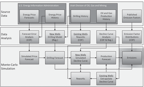
The overall structure of the model is summarized in Figure 1. Each step in the data analysis and Monte Carlo (MC) simulation are discussed in detail in subsequent sections. In summary, source data primarily from the U.S. Energy Information Administration (EIA) and Utah Division of Oil, Gas and Mining (DOGM) are collected and analyzed to find either (a) a cumulative distribution function (CDF) or (b) a least-squares regression fit to the following model input parameters:

1. Forecast error (CDF): The range of relative error between actual energy prices and EIA energy price forecasts.

2. Drilling model (regression): A fitted model that predicts the number of new wells drilled in response to current and/or past energy prices.

3. Reworks (CDF): The probability that existing wells will be reperforated or recompleted as a function time.

4. Decline curve analysis (CDF and regression): Production from all wells tends to decrease over time. Individual decline curves are fitted using nonlinear least-squares regression to the unique production histories of every well in the Uinta Basin. Then, the range of values of the fitted decline curve coefficients are described using CDFs.

5. Emission factors (CDF): The range of emission factors for various oil and gas drilling and production activities are modeled as a normal distribution based on the mean and standard deviation of reported emission factors we collected in a literature review.

Figure 1. Diagram of the emission model.

After analyzing the source data, a MC simulation is then run to determine the distribution of possible emissions inventory outcomes. The following algorithm is executed for each iteration (i.e., run) of the MC simulation:

1. Generate a simulated oil and gas price forecast. EIA forecasts are used as a basis and are adjusted up or down based on the CDF of forecasting error. Price forecasts are interpolated from an annual to a monthly basis (the time step used in rest of the MC simulation).

2. Calculate the number of new wells drilled in response to simulated energy prices by using the fitted drilling model. Additionally, randomly draw from the rework CDF to determine if and when a rework event will occur for each new and existing well.

3. For every well (new and existing):

   1. Pick/collect well attributes (well depth, decline curve coefficients, emission factors, etc.). Attributes for new wells are randomly picked by selecting from CDFs created in the data analysis step. Existing wells use their actual (or fitted) attributes.

   2. Calculate production rates of oil and gas for each well. Production from existing wells is found by extrapolating from each well’s individually fitted decline curves. Production from new wells is calculated using the randomly picked decline curve coefficients generated in the previous step.

   3. Calculate emissions from one-time (drilling, completions, reworks) and ongoing (production, processing, etc.) events. Emissions are calculated by multiplying each randomly selected emission factor (for each well and for each emission activity type) by that factor’s quantity of interest (i.e., the date for one-time events such as completion, or the amount of oil or gas produced).

4. Sum together results for all wells to find the total emissions inventory for given run of MC simulation.

By repeating the above algorithm many times (≥10⁴ iterations) and randomly drawing from the CDFs for each input parameter (where applicable), a representative sample of all possible emissions inventory outcomes is generated. The range of MC simulation results can then be analyzed to determine the probability of possible outcomes, clearly quantifying the uncertainty in the model’s results.

All data analysis and MC simulation steps are written in R (R Core Team, 2015), which allows for the entire model to be run automatically in either a “cross-validation” or “predictive” mode. In the cross-validation mode, the available data are separated into two time intervals. Data in the first interval, referred to as the “training” period, are used to generate all of the input parameter CDFs and regression fits. The MC simulation is then run over the second time interval. Data points in the second “testing” time interval can then be used to gauge the accuracy and validity of the MC simulation results. In the predictive mode, the model is trained using all available data, and the MC simulation estimates emissions for a future time period.

The details of each step in the data analysis and MC simulation process are discussed further below.

Energy price forecast

The first step of the MC simulation is generating a set of simulated energy price forecasts for the first purchase price (FPP) oil and gas prices. We use the U.S. EIA’s Annual Energy Outlook (AEO) forecasts (U.S. EIA, 2015b) for wellhead oil and gas prices in the Rocky Mountain region as the basis for our forecasting work. Although EIA’s AEO forecasts are frequently used as a standard estimate for future energy prices, they are also frequently wrong, with prices being off by as much as ±100% of their actual value after just 5 yr (U.S. EIA, 2015a). The range of possible error in EIA forecasts must be included in the simulated energy price forecast to propagate that uncertainty into emissions inventory estimates. We calculated the relative error between actual FPPs of oil and gas in Utah and EIA’s forecasted prices over the 1999–2014 time period (the full time period for which Rocky Mountain wellhead price forecasts were included in AEO reports) using eqs 1 and 2:

(1)

(2)

where RE is the relative error between the forecasted price FP and the actual price AP. Defining RE this way is useful because

1. The value of RE is always bounded between 0 and 1 and can be described using a beta probability distribution.

2. It captures the absolute magnitude of the relative error. Although EIA underpredicted actual FPPs for oil over the 1999–2007 time period, forecasts from 2009 onwards have overpredicted actual FPPs for oil (gas prices have followed a similar pattern). There is no evidence that EIA’s forecasts are systemically under- or overpredicting energy prices.

3. Equations 1 and 2 avoid a mathematical pitfall that occurs with a simple absolute value calculation of RE. Suppose that RE was defined as

(3)

Substituting the simulated price (SP) for AP and rearranging gives:

(4)

If a negative value of RE is selected during the MC simulation process, SP may be negative, which is not a realistic result. By comparison, solving eqs 1 and 2 always returns a result bounded between [0, +∞]:

(5)

(6)

Figure 2 shows a boxplot of the distribution of values for RE for oil and gas by future-year (i.e., how far into the future the forecast is) calculated according to eqs 1 and 2.

Figure 2. Boxplot of relative error between actual FPPs of (a) oil and (b) gas versus EIA AEO wellhead oil and gas prices in the Rocky Mountain region as calculated by eqs 1 and 2.

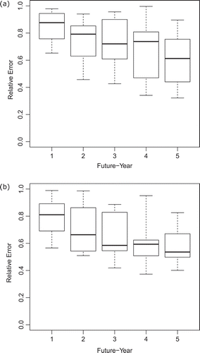
A beta distribution with shape parameters α and β was fitted to the empirical distributions of RE values in Figure 2, resulting in the parameter values given in Table 1. The beta distribution was selected to model values of RE because it’s a continuous probability distribution bounded between 0 and 1 (the same range of values possible for RE using eqs 1 and 2). These shape parameters are used to create two theoretical CDFs for RE by future-year, one for oil and one for gas. During the MC simulation, percentiles of these two CDFs are randomly selected, and then the percentiles are traced through the two CDFs by future-year. For example, if the 50th (median) percentile were selected for gas, the values of RE would be 0.81, 0.75, 0.66, 0.62, and 0.58 for future-years 1 through 5. The value for SP is then calculated using either eq 5 or 6 with an FP value obtained from the EIA AEO forecast. Which form of the equation to use is also selected randomly (with equal probability). Lastly, both the EIA AEO forecasts and the RE CDFs are converted from an annual basis to a monthly basis using linear interpolation, since all other components in the modeling process are calculated on a monthly basis.

Table 1. Relative error beta distribution shape parameters α and β for oil and gas by future-year.

ForecastType	Future-Year	α Parameter	β Parameter	R^2	DataPoints
Gas	1	6.214	1.666	0.988	16
Gas	2	3.034	1.212	0.875	15
Gas	3	5.330	2.859	0.897	14
Gas	4	4.575	2.937	0.887	13
Gas	5	8.047	5.995	0.908	12
Oil	1	8.650	1.507	0.976	16
Oil	2	5.549	1.975	0.974	15
Oil	3	4.185	1.642	0.949	14
Oil	4	2.345	0.998	0.957	13
Oil	5	4.736	3.058	0.976	12

Drilling forecast

Forecasting drilling activity is a key part of estimating overall emissions in the Uinta Basin because new wells are (a) responsible for the overall growth rate of oil and gas production in the region and (b) are major sources of one-time emissions. Drilling activity can occur either in the form of drilling new wells or “reworking” existing and/or abandoned wells to stimulate new production. The methods used for forecasting each type of drilling activity are discussed below.

New wells

The number of wells drilled each month in the Uinta Basin can be modeled as a function of energy prices using a variety of distributed lag models. We tested four different distributed lag price models:

(7)

(8)

(9)

(10)

where W is the number of new wells drilled at time t, OP is the FPP of oil in dollars per barrel ($/bbl), GP is the FPP of gas in dollars per thousand cubic feet ($/MCF), and all other terms (a, b, c, and d) are coefficients fitted using linear regression. Data on the number of wells drilled (Utah DOGM, 2015) and the values of OP and GP in the Uinta Basin (U.S. EIA, 2015c, 2015d) were used to find the best fit for each model over the time period of January 1995–December 2009 (the training period) and were cross-validated against data from the January 2010–December 2014 time period (the test period). Results for the training fit and cross-validation test are summarized in Table 2 and plotted in Figures 3 and 4.

Table 2. Distributed lag drilling model fit (training period 1995–2009) and cross-validation (test period 2010–2014) results.

	Coefficient
DistributedLag Model	a	b	c	d	TrainingPeriod R^2	TestPeriod RSS
Equation 7	0.072	0.742	0.867	−1.987	0.865	4.50E+04
Equation 8	0.590	3.382	−6.889		0.736	2.53E+04
Equation 9	0.844	−1.451			0.699	9.31E+03
Equation 10	8.293	−4.923			0.609	1.33E+05

Notes: “Test period RSS” refers to the residual sum of squares during the cross-validation test period.

Figure 3. Training fit of distributed lag drilling models eqs 7–10. Actual drilling (Utah DOGM, 2015) and energy price (U.S. EIA, 2015c, 2015d) histories from January 1995 to December 2009 were used to find the best fit for each model using least-squares regression.

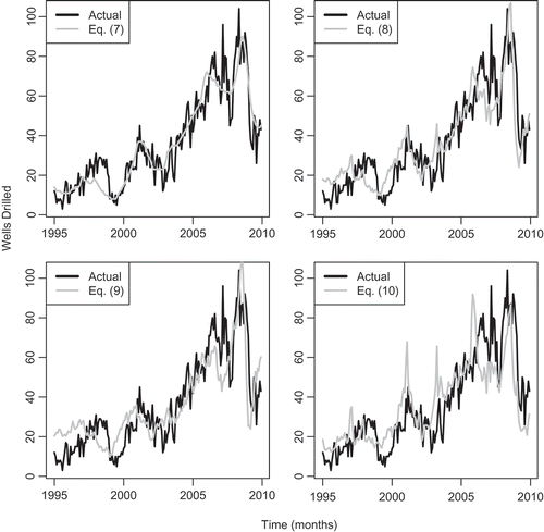
Figure 4. Cross-validation test of distributed lag drilling models eqs 7–10. Each model was tested against actual drilling (Utah DOGM, 2015) and energy price (U.S. EIA, 2015c, 2015d) histories from January 2010 to December 2014.

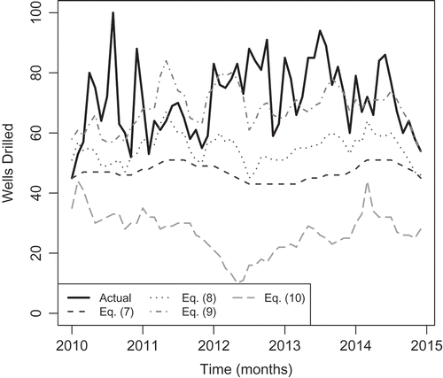
In general, all of the distributed lag models fit the drilling record from 1995 to 2009 reasonably well. The correlation between energy prices and drilling activity in the Uinta Basin is particularly strong after 2000. Equation 7 gives the best fit during the training period because (a) the prior well term dampens the effect of monthly energy price fluctuations on drilling activity and (b) eq 7 contains more fitted terms. Equations 8–10 all underpredict drilling rates from 2006 to 2007, particularly eq 10 (which also fails to follow the spike in drilling in 2008 due to higher oil prices). Although eq 7 would appear to be the best model, the cross-validation results shown in Figure 4 and Table 2 both reveal that eq 7 fails to respond to the energy price changes in the 2010–2014 time period, indicating that the model is most likely overfitted to the training period’s drilling and energy price history. Equation 8 performs slightly better than eq 7, and eq 10 fails completely. Overall, drilling activity in the Uinta Basin over the last 20 yr (and especially the last 15 yr) has been closely correlated with oil prices, and the fit and cross-validation of eq 9 demonstrate that a simple distributed lag model based on oil prices is sufficient for estimating future drilling activity in the Uinta Basin. As a result, eq 9 was selected for use in estimating the number of new wells drilled in the MC simulation.

In addition to determining how many new wells are drilled, the geographical location and type of well (oil or gas) must also be selected. We assume that the geographical distribution of new wells (i.e., what oil or gas field a new well will be located in) and the ratio of oil wells to gas wells (which is location specific) can both be described by empirical CDFs based on historical data (Utah DOGM, 2015), and that the well type ratio in a given location is constant. It should be noted that well type merely indicates what type of product (oil or gas) is predominantly produced by a well. In reality (and in the simulation), all wells produce both oil and gas.

Reworked wells

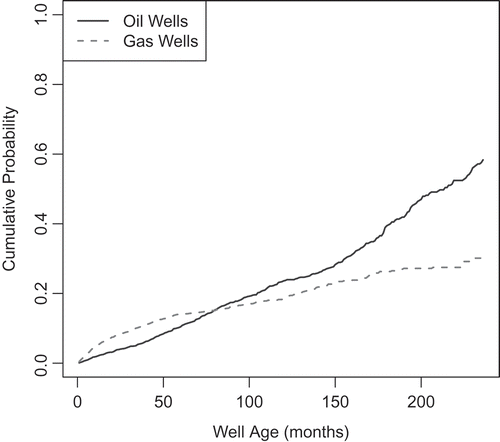
Reworks are drilling events where an existing well is either recompleted or reperforated to stimulate oil and gas production rates. Reworks have a large impact on emissions both because (a) reworking a well is a large one-time source of fugitive emissions and (b) production rates usually rise dramatically after reworks. The timing of rework events are estimated using an empirical CDF, based on 1137 rework events listed in the Utah DOGM (2015) database to describe the probability that a well is reworked based on (a) well type (oil or gas) and (b) how long the well has been in operation, as shown in Figure 5. For each MC simulation run, every well (new and existing) randomly draws a rework date from the CDFs in Figure 5. Note that rework dates can be selected that are outside of the simulation time frame. For example, if a well that is 50 months old at the start of a 60-month (5-yr) simulation draws a rework time that is earlier than 50 months or later than 110 months, the rework event for that particular well is effectively ignored.

Figure 5. Well rework CDF describing probability of a well having at least one rework event based on (a) well age and (b) well type (oil or gas).

Production forecast

n general, production rates of oil and gas from any well decline over time. Arps (1945) proposed a set of empirically based “decline curve” equations to estimate a well’s future production rates based on its rate of decline. Subsequently, the theoretical basis for decline curves has been established by other authors (Doublet et al., 1994; Fetkovich et al., 1996; Shirman, 1998; Ling and He, 2012; Okouma Mangha et al., 2012). Numerous decline curve equations have been developed for specific oil and gas reservoir conditions. The two forms of decline curve equations used here are the hyperbolic decline curve equation (eq 11; Arps, 1945) and the cumulative production equation (eq 12; Walton, 2014):

(11)

(12)

In eq 11, q is the oil or gas production rate at time t, q_o is the initial production rate, b is the decline exponent, and D_i is the initial decline rate. In eq 12, Q is the cumulative production at time t, and C_p and c₁ are fitted coefficients. Equations 11 and 12 are fitted to the oil and gas production records of every unique well in the Uinta Basin (Utah DOGM, 2015) using nonlinear least-squares regression. The fits found for eq 11 are then extrapolated to estimate the future production for all existing wells, whereas the fits for eq 12 are used to generate CDFs for use in simulation the production rates of new wells. Production from new wells is estimated using eq 12 because monthly production rates (calculated by difference from the value of Q) are a function of only a single fitted coefficient, C_p, as opposed to three coefficients (q_o, D_i, and b) in eq 11. Random and independent draws from the CDFs for the coefficients in eq 11 almost always return unrealistic results (e.g., thousands of wells with no production, then a single well with higher production rates than the entire Uinta Basin combined). However, the fits for eq 11 are frequently more accurate at longer time periods than eq 12. Therefore, eq 11 is preferred for estimating the production rates for existing wells.

Unfortunately, many wells have complicated production histories (shut-ins, workovers, water-flooding, etc.) that prevent easy fitting. To overcome this problem, we developed an algorithm that automatically identifies the start and stop points of distinct decline curves in each well’s production records and then fits eqs 11 and 12 to each curve separately. An example of this approach is shown in Figure 6.

Figure 6. Decline curve analysis fitting (a) eq 11 to monthly oil rates and (b) eq 12 to cumulative oil production from an oil well in the Uinta Basin (API no. 43-013-31123). Dashed lines indicate the time index identified as a start/stop point by the algorithm responsible for finding distinct decline curve segments. Both the hyperbolic and cumulative curve fits use the same start/stop points. If only a single curve is found, then that curve counts as both the “first” and “last” curve. The production segment at the very beginning (t < 24 months) is ignored by the algorithm because some wells have short and sporadic decline curves during their first few years of operation.

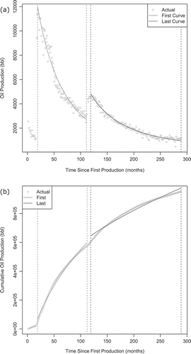
Only the fits of the “first” and “last” curve segments are saved. If only a single curve is found, then that curve is counted as both the “first” and “last” curve. The production rates of existing wells are calculated directly from the “last” fits of eq 11 for each existing well (for both oil and gas). Production of oil and gas from new wells can be simulated by either one of the following:

1. Randomly picking coefficients for eq 12 from the empirical CDFs of fitted coefficients from the “first” curves. This method works well if new wells are expected to have the same production rates as existing wells.

2. Utilizing log-normal distribution fitting to account for changing trends in the production rates of new wells. Specifically:

   1. Fit a log-normal distribution to values of C_p and c₁ by year.

   2. Use linear regression to fit the log-normal distribution shape parameters, log-mean and log-standard deviation (SD).

   3. Extrapolate from fitted log-mean and log-SD trend-lines to estimate the distribution of C_p and c₁.

Given recent production trends, we have found that gas production from new wells is best simulated using the empirical CDF method, whereas oil production from new wells is most successfully handled by using the log-normal distribution method.

There are several other important caveats to the production forecast as detailed below.

Existing wells without decline curve fits

In total, applying the curve fitting algorithm to the 12,071 unique wells in the Uinta Basin results in approximately 48,000 unique curve fitting attempts (both oil and gas production records for each well using both eqs 11 and 12). The algorithm is fairly robust; only 4% of the attempted fits fail to find a fit. However, 22% of the wells are skipped because they contain too few (<12 months) nonzero production records. Existing wells without fits are treated using the same methodology applied to new wells.

Production impact of well reworks

As discussed previously, reworking a well usually results in substantially increased production rates. To model the effect of reworks, any well that is randomly selected for rework is treated as a new well from the time step that the rework occurs. For example, if an existing well that was 40 months old at the beginning of the simulation is scheduled for a rework in month 10 of a 60-month long simulation period, production for months 40–49 would occur according to the original decline curve (eq 11), whereas production for months 50–99 would be computed using eq 12 with a randomly selected set of coefficients.

Well abandonment

Eventually, the decline in a well’s production rates will become so low that it becomes uneconomical to continue to operate. To correct for wells that are producing at uneconomical rates, the last step in the production forecasting process is to estimate each well’s operating cost ratio CR as a function of time:

(13)

where LOC is the lease operating costs (pumping, labor, maintenance, etc.) for the well and GR is the gross revenue from oil and gas sales. LOC is estimated from EIA (2010b) data based on well type, depth, energy prices, and production rates, giving the following linear regression fits:

(14)

(15)

where q_gas is the monthly production rate of gas (MCF/month), D is well depth (in ft.), and “oil” and “gas” subscripts denote well type. The fit given in eq 14 is based on 64 data points (R² = 0.982) and eq 15 on 160 data points (R² = 0.927), which represent all of the available LOC data for both well types from EIA (2010b). Any well which is found to have a CR(t) ≥ 0.8 is assumed to be shut-in and permanently abandoned (since approximately 15% of GR is paid in royalties and severance taxes).

Emissions

Given the uncertainty in reported emission factors for the oil and gas industry, we elected to use the same approach applied to other input parameters in our model to compute emissions from oil and gas development; namely, we described emission factor ranges using CDFs and from the CDFs (for each well) randomly selected the emission factor values to apply to the drilling and production forecast. The details of implementing this approach to calculate total emissions are described below.

Emission factor sources

This study groups emission factors for greenhouse gases (GHG), methane (CH₄), and volatile organic compounds (VOCs) into the categories that correspond to the process steps: site preparation; material transport; well drilling; fracturing and completion (including flowback); production; product processing; and product transport. Emission factors were estimated from a review of published studies aimed at emissions from oil and gas operations with an emphasis on the Uinta Basin and tight-gas/tight-sand formations. Methane emissions were converted to CO₂ equivalents (CO₂e) on a 100-yr time frame (using a global warming potential of 21), and nitrous oxide (N₂O) emissions were converted to CO₂e using a global warming potential of 310 (Intergovernmental Panel on Climate Change [IPCC], 2007). VOC emissions were estimated using the ratio of VOCs to CH₄ at the wellhead in the Uinta Basin from Zhang et al. (2009) (CH₄ 75%, VOCs 12%) and from U.S. Environmental Protection Agency’s (EPA’s) smoke model (55% methane and 33% VOCs) (University of North Carolina at Chapel Hill, 2014). The composition difference between Zhang et al. and EPA’s smoke model was considered as part of the emission-factor uncertainty.

For the same process steps, emission factors can vary by orders of magnitude. These differences are most likely due to different conditions at the study sites and different study methods. For example, formation properties and well productivity affect emissions. In addition, the emission factors come from different types of studies: surveys, emission measurements made on individual operations or pieces of equipment, and regional (top-down) measurements. The survey-based studies tend to report lower emissions than the other two types. Furthermore, the measurements at individual locations may not be representative of the operations from the entire region. For example, Karion et al. (2013) performed a top-down study and estimated that between 6.2% and 11.7% of natural gas produced is emitted in the Uinta Basin, whereas Pétron et al. (2012) estimated losses of 1.7–7.7% from the Piceance Basin. These top-down estimates are significantly higher than emissions estimated from survey-based emission factors (Western Regional Air Partnership, 2008) or other inventories (EPA, 2013; Utah State University, 2013). Recent modeling studies by Ahmadov et al. (2015) suggest that the Karion estimate may be in the correct range. However, because many of the oil and gas producing regions also have natural gas seeps, it can be difficult to resolve natural gas production activities from naturally occurring sources of CH₄ and VOCs.

Emission factor values

Table 3 provides the average and standard deviation of emission factors by process. Assuming that all of the emission factors follow a normal distribution, the mean and SD values in Table 3 can be used to generate CDFs for each factor. Emission factors are assumed to follow a normal distribution because of the limited number of data points available.

Table 3. Best estimates of emission factors for the Uinta Basin prior to implementation of EPA’s New Source Performance Standards (NSPS) and new state rules on pneumatic controllers.

Activity	CO2e	CH4	VOCs	Units	Data Points
Site preparation (excluding drill rig transportation)^a	208 ± 79	9.9 ± 3.37	1.58 ± 0.60	10^3 kg/well	3
TM drilling^b	0.40 ± 0.56	8.6E-06 ± 1.22E-05	1.38E-06 ± 1.95E-06	10^3 kg/well	—
TM completions^b	0.21 ± 0.29	4.36E-06 ± 6.16E-06	6.97E-07 ± 9.86E-07	10^3 kg/well	—
TM rework^b	3.05 ± 4.31	7.71E-05 ± 1.01E-04	1.15E-05 ± 1.62E-05	10^3 kg/well	—
TM production^b	1.36 ± 1.93	3.29E-05 ± 4.65E-05	5.26E-06 ± 7.43E-06	10^3 kg/well	—
Well completion^c	1940 ± 967	92.4 ± 46	14.8 ± 7.37	10^3 kg/well completion	4
Gas production^d	43 ± 40	2.07 ± 1.90	0.78 ± 0.73	10^3 kg/yr well	10
Gas processing^e	901 ± 46	5.58 ± 3.91	0.89 ± 0.62	10^3 kg/10^9 ft^3 of total natural gas production	4
Gas transmission and distribution^f	4177 ± 3423	199 ± 163	31.8 ± 26	10^3 kg/10^9 ft^3 of total natural gas production	10

Notes: TM = transportation of materials. ^aCorresponds to the average of the emission factors by Jiang et al. (2011) and Santoro et al. (2011). ^bCalculations based on a study of transportation emissions in the Piceance Basin of Northwestern Colorado (Bar-Ilan et al., 2011). ^cThis value corresponds to the average of the emission factors reported by O’Sullivan and Paletsev (2012) for tight oil wells, Skone et al. (2014) for tight gas wells, American Petroleum Institute (2012) for the Rocky Mountain region, and Allen et al. (2013) for the Rocky Mountain region. Skone et al. assume that tight gas well completion emission factor is 40% of the emission factor for shale gas wells completion. This value includes both controlled and uncontrolled emissions. ^dRocky Mountain region (Allen et al., 2013). This value includes both controlled and uncontrolled emissions. ^eAverage of the emission factors reported by Burnham (2011), Jiang et al. (2011), Skone et al. (2014), and Canadian Association of Petroleum Producers (1999). This value includes both controlled and uncontrolled emissions. The contribution of CH₄ to the CO₂e emissions from processing activities before NSPS implementation was estimated to be around 13% (Skone et al., 2014). This same percentage was applied to estimate the CH₄ contribution from processing activities. ^fCorresponds to the average of emission factor values reported by Howarth et al. (2011) for several studies. These values include both controlled and uncontrolled emissions.

Table 4 presents the emission factors for CO₂, CH₄, and VOC emissions from the production and transport of oil. Since only a single source was found for estimating these factors, the normal CDF for these emission factors is generated assuming that the mean and standard deviation are both equal to the values given in Table 4. This study further assumes that the emissions from site preparation, drilling, fracturing, and completion for oil wells are the same as those reported for gas wells.

Table 4. Emission factors for oil production and transport from Picard (2000).

Activity	CO2e	CH4	VOCs	Units
Production^a	4.91E-05	2.34E-06	8.88E-07	10^3 kg/ bbl
Transport^b	1.15 E-03	2.82E-07	3.84E-07	10^3 kg/bbl transportedtanker truck

Notes: ^aAverage of reported emission factors ranging from conventional to heavy oil. VOCs are estimated from Zhang et al. (2009) (CH₄ 75%, VOCs 12%) and from the EPA smoke speciate composition (55% CH₄ and 33% VOC). The standard deviation includes the two different compositions. ^bCO₂, CH₄, N₂O, and VOC emissions for Heavy-Heavy Duty Truck from GREET 2014 (Argonne National Laboratory, 2014). CO₂e estimated for global warming potential of 1 for CO₂, 21 for CH₄, and 310 for N₂O (IPCC, 2007). The average distance from the oil reservoirs to the geographic edge of the Uinta Basin along the most common trucking route is 121 miles. Crude oil is assumed to be carried by trucks with an average capacity of 200 barrels (HDR Engineering, 2013).

Calculation of emissions

The emission categories from Tables 3 and 4 are simplified into one-time events (drilling, reworking, and completing a well) and ongoing emissions (from production and transportation of produced oil and gas). The largest one-time emission source is completion, which is assumed to occur every time a well is drilled or reworked. Emissions from completion are tracked separately from the rest of the drilling and reworking activity. Noncompletion-related emissions for drilling are assumed to be the sum of the emission factors for site preparation and transportation of materials for drilling, completion, and production. Noncompletion rework emissions are assumed to be the sum of emission factors for transportation of materials for completion and reworking. The drilling schedule then determines the quantity and timing of all one-time emission events. All of the ongoing emissions are calculated directly from the production schedule by multiplying production volumes by the per unit volume emission factors specified in Tables 3 and 4.

Effect of new regulations

The EPA recently finalized New Source Performance Standards (NSPS) for the oil and natural gas sector (EPA, 2012). Table 5 summarizes the effect of the NSPS on emission factors and their implementation schedule.

Table 5. Change in emission factors for CO₂e, CH₄, and VOCs after the NSPS implementation for new wells (NETL 2014).^a

Process	CO2e (%)	CH4 (%)	VOCs (%)	Beginning
Construction	+2	—	—	January, 2015
Completion	−96	−96	−96	January, 2015
Production	−66	−66	−66	November, 2012
Processing	−20	−40^b	−40^b	November, 2012
Transport^c	−0.5	−0.5	−0.5	November, 2012

Notes: ^aThe beginning dates are the effective dates of NSPS. Some of the categories, such as production, encompass several activities, such as pneumatic controllers and workovers. In this case, the beginning date is the date of the largest contributor to the category. ^bBased on the Skone et al. (2014) data. Value assumes that emissions from other point sources and valve fugitives are mainly due to methane. ^cBased on the Skone et al. (2014) data. Methane emitted due to pipeline construction was not included.

Additionally, beginning in 2015, new state rules require the replacement of existing high-bleed pneumatic control devices with low-bleed devices. These rules apply to oil and gas operations on state and federal lands but not to operations tribal lands. The pneumatic controller regulations will result in a 1.2% reduction of all VOC and CH₄ emissions for Uinta County and an 11% reduction for Duchesne County (Oswald, 2015).

All of these reductions are implemented in the model by reducing the base emissions calculated from Tables 3 and 4 by the percentages specified in Table 5 and in the state pneumatic controller rules. The November 2012 NSPS in Table 5 is applied only to new gas wells. The January 2015 NSPS impact on construction is applied to all wells and very slightly increases the emissions related to the transportation of materials for drilling and the drilling activity itself. The January 2015 NSPS applies to all completions and reworks. The pneumatic controller regulations are implemented by reducing all VOC and CH₄ emissions by the overall reductions for each county.

Results and Discussion

Two sets of results are shown below for running the model in (a) cross-validation mode and (b) predictive mode. The cross-validation run presents the results of training the model with data from 1984–2009 and then testing the model against data from the 2010–2014 time period. The predictive run uses all of the available data (1984–2014) to predict emissions over the 2015–2019 time period. The range of results shown for both runs were obtained by performing a MC simulation with 10⁴ iterations.

Energy price forecasts

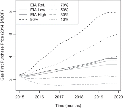
Simulated energy price forecasts for oil and gas FPPs are shown in Figures 7 and 8 for the cross-validation and prediction cases, respectively. Dotted lines represent various percentiles of simulation results (10th percentile, 20th percentile, etc.), whereas the solid black lines show the actual oil and gas price paths. Additionally, the reference and outlier (highest price/lowest price) forecasts from EIA’s AEO reports are shown as shaded-gray lines. The cross-validation case uses EIA’s AEO 2010 report (U.S. EIA, 2010a) as a basis, whereas the prediction case uses AEO 2015 (U.S. EIA, 2015b).

Figure 7. Simulated energy price forecast for the cross-validation case for (a) oil and (b) gas FPPs. Various percentiles of results are shown as dotted lines, actual prices as solid black lines, and EIA AEO 2010 (U.S. EIA, 2010a) price forecasts as gray scale lines.

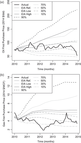
Figure 8. Simulated energy price forecast for the prediction case for (a) oil and (b) gas FPPs. Various percentiles of results are shown as dotted lines, actual prices as solid black lines, and EIA AEO 2015 (U.S. EIA, 2015b) price forecasts as gray scale lines.

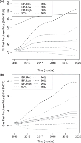
In general, the simulated energy price paths (a) cover the range of observed prices, (b) meet or exceed the range of variability in EIA’s extreme price forecasts, and (c) have a median (50th percentile) result that closely follows the reference forecast. There are some exceptions. Actual gas prices in Figure 7b drop below even the 10th percentile of the simulated forecast during 2012. Additionally, the median simulated price forecasts for gas in Figures 7b and 8b are lower than the EIA reference gas forecast. Whether a forecast under- or overpredicts is determined by randomly drawing from a binomial distribution, with each outcome having equal probability. With the specified random number generation seed, the binomial draws result in a nearly even split of under- and overpredictions for oil prices but a skew towards underpredictions for gas prices. Since the cross-validation and prediction cases use the same probability draw sequence, the same result appears in both Figures 7b and 8b. Repeated tests with different random number seeds and varying numbers of MC simulation iterations have shown that whereas the directionality of the error for the median case can change, all of the other percentiles are relatively stable (e.g., there is almost no change in the distribution of the forecast results between 10⁴ and 10⁵ MC simulation iterations; see Figure 9).

Figure 9. Simulated energy price forecast for the prediction case for gas FPPs using the same random number generation seed as Figures 7b and 8b, but with 10⁵ MC simulation iterations instead of 10⁴ iterations. Since the number of random draws changes, the directionality of the under/overprediction changes for the median case; however, the other percentile results are nearly identical between the two sample sizes.

Drilling forecasts

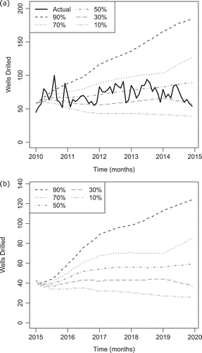
Applying eq 9 to the simulated price forecasts in Figures 7 and 8 produces the drilling forecasts presented in Figure 10 for the (a) cross-validation and (b) prediction cases. In cross-validation mode, the median drilling forecast over the 60-month period shown in Figure 10a (total of 4486 wells) is a reasonable match for the actual drilling schedule (total of 4272 wells). In prediction mode, lower energy prices result in reduced drilling activity (median case has total of 3121 wells).

Figure 10. Drilling forecast for the (a) cross-validation and (b) prediction cases.

Production forecasts

Several production forecasts for different cases and assumptions are shown in Figures 11–14. Figure 11 shows monthly oil production rates from (a) new wells and (b) existing wells, as well as the monthly gas production rates from (c) new wells and (d) existing wells, for the cross-validation case. The median result for oil production from new wells is an excellent match for the actual oil production from wells drilled during the 2010–2014 time period (73.1E+06 bbl simulated versus 71.9E+06 bbl actual). Simulated gas production from new wells is a good match to the actual production rate until 2013, at which point the median simulated gas production rate continues to increase, whereas the actual gas production rate decreases. However, the actual gas production rate from new wells is still fully covered within the 10th–90th percentile interval. Oil and gas production from existing wells is also a reasonably close match (simulated production of 46.2E+06 bbl oil and 941E+06 MCF gas versus actual production of 47.3E+06 bbl oil and 956E+06 MCF gas), although there is a small but clear trend to underpredict production at the beginning and overpredict production at the end of the simulation period. The under/over trend is due to well reworks; as more time passes, it becomes increasingly likely that a larger portion of the existing well population will be reworked (boosting production rates from reworked wells). However, neglecting reworks (by setting the rework probability to zero) leads to a substantial underprediction of production rates from existing wells (especially oil wells); see Figure 12.

Figure 11. Production forecast for the cross-validation case for (a) oil production from new wells, (b) oil production from existing wells, (c) gas production from new wells, and (d) gas production from existing wells.

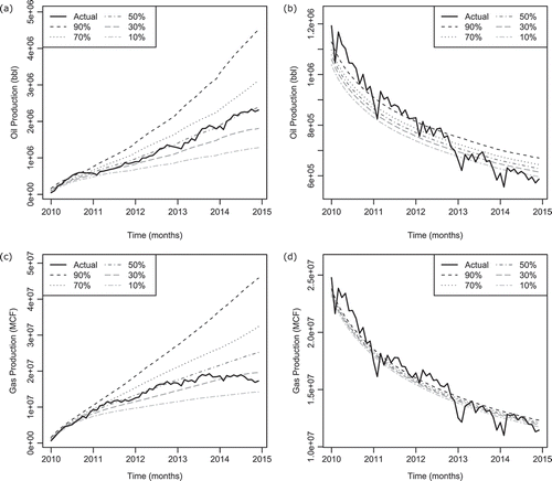
Figure 12. Production forecast for the cross-validation case for production of (a) oil and (b) gas from existing wells assuming no well reworks occur.

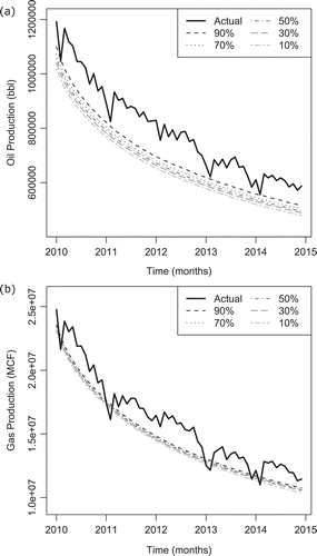
Figure 13. Production forecast for the cross-validation case for (a) oil and (b) gas production from new wells taking the actual drilling schedule as a given.

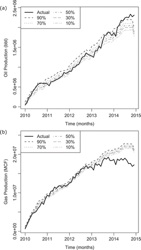
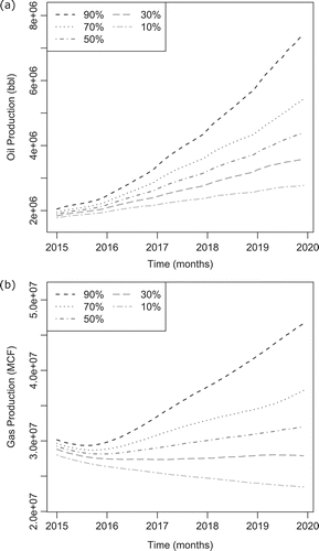
Figure 14. Production forecast for the prediction case for (a) oil and (b) gas production from all (new and existing) wells.

Almost all of the variability in the production forecasts stems from the uncertainty in the drilling forecast (and its antecedent, the energy price forecast). Figure 13 shows the production rates of oil and gas from new wells if the actual drilling rates during the simulation period are taken as a given (i.e., the total number of wells drilled in each month is used for W instead of simulating W using eq 9). Effectively, Figure 13 shows just the variability in production rates that stems from the random selection of (a) well location, (b) well type (oil or gas wells), and (c) decline curve coefficients from eq 12. Production rates in Figure 13 are nearly an exact match to actual production rates except for gas production after 2013. Given the close match between simulated versus actual gas production from 2010 to 2013, the discrepancy from 2013 to 2015 is due to (a) the well rework probability and (b) a drop in the actual number of gas wells being drilled. Assuming zero rework activity only partially reduces the discrepancy (median simulated gas production rates assuming no reworks is approximately 20E+06 MCF/month vs. the actual rate of 17.3E+06 MCF/month). As for the second cause, well location and type have certainly changed in the Uinta Basin over time, so there is likely some error introduced by the assumption that the location and type of new wells will follow the same pattern as past wells. Over the time period of 1984–2009, 53% of new wells in the Uinta Basin were gas wells; however, during the time period of 2010–2014, that fraction dropped to 36%.

The total oil and gas production from all wells (new and existing) is shown in Figure 14 for the prediction case. Interestingly, even though fewer oil wells are drilled in the prediction case (as a consequence of the reduced energy price forecast) than in the cross-validation case, oil production rates nearly double. The higher oil production rate is a consequence of extrapolating the increased production rates that the industry has demonstrated over the last decade via the log-normal trend-line fitting method discussed in Production Forecast. Gas production rates, which are modeled using the empirical CDF method (and therefore assume that new gas wells will show the same production histories as previously drilled wells), increase more slowly over most of the simulation period.

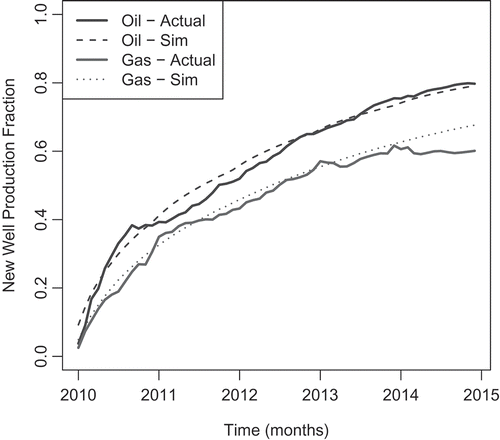
Lastly, it is interesting to note how much production occurs from new wells versus existing wells. Figure 15 shows the fraction of production that is attributable to new wells for both oil and gas production in the cross-validation case for the simulated production forecast (median results) versus the actual production history. Presumably new wells could be required to adhere to higher emission standards than existing wells, which over time would drop out of production. The point at which new wells become responsible for more than 50% of the overall production is about 2 yr for oil and 3 yr for gas.

Figure 15. Fraction of total production that is generated from new wells as a function of time for the cross-validation case. Simulated results are shown as dotted lines and the actual production history as solid lines.

Emissions

Of the three types of emissions calculated by the model, VOCs are currently the top regulatory concern. Therefore, only the results for VOC emissions are discussed in detail below. However, since VOC emissions are calculated as a ratio of CH₄ emissions, all of the results and trends noted below are similar for the other two emission categories (usually with just a change in scale on the y-axis). The results for CO₂e and CH₄ emissions are provided as supplemental figures.

VOC emissions calculated by applying the emission factors to the drilling and production forecasts are shown in Figures 16 and 17 on a monthly and annual basis, respectively. Both figures indicate the baseline and reduced emissions (as a result of implementing NSPS and state rules) for the cross-validation and prediction modes. As shown in Figures 16a and 17a, there is very little reduction in VOC emissions as a result of implementing the November 2012 NSPS rules in Table 5, since these emissions are only applied to newly-drilled wells and the emission reductions are not applied to the largest emission categories (completions and gas transmission). The reductions that occur starting January 2015 have a much larger impact, as illustrated in Figure 16b. With these control reductions, emission rates remain flat at around 2000 metric tons/month for the entire prediction period (nearly 50% lower than the base-level emissions). Figure 17 gives a breakdown of emissions by source on an annual basis, and shows that the majority of the emissions are due to completion events, followed by gas transmission and gas production. As with Figure 16b, Figure 17b illustrates the impact of the emission reductions and in particular of the EPA green completion rule, which dramatically decreases emissions from the completion category.

Figure 16. VOC emission percentile results for the (a) cross-validation and (b) prediction cases. Base emissions are shown as solid gray-scale lines, and reduced emissions from NSPS and state rules are shown as dotted lines.

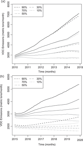
Figure 17. Total median (50th percentile) VOC emissions for the (a) cross-validation and (b) prediction cases. Results are shown by year (Y1, Y2, etc.) and source for baseline emissions (B) and reduced emissions (R). Activities in the “Other” category include reworking, gas processing, oil production, and oil transportation.

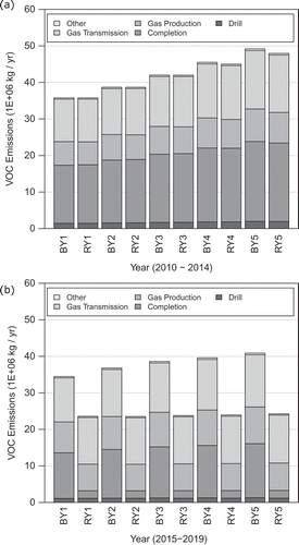
Comparing final emission results at the end of the cross-validation case (2014) in Figure 17a to the start of the prediction case (2015) in Figure 17b, we can see that there in an almost 25% reduction in median baseline emissions. The disparity is due to the differences in drilling and production rates at the end of the cross-validation case period (December 2014) versus the beginning of the prediction case period (January 2015). The step change indicates both the sensitivity of emission rates (in the model and in reality) to the oil and gas industry’s business cycle and the importance of the uncertainty quantification. The starting point of the prediction period’s median VOC emissions is equivalent to the 15th percentile of the cross-validation cases VOC emissions in December 2014.

Conclusions

In this study, we demonstrated a method for estimating (with uncertainty) the drilling, production, and emissions inventory of the oil and gas industry in Utah’s Uinta Basin. In cross-validation tests, the median simulation results have proven to be highly accurate at matching the test history data. Assuming that the emission factors found in our literature review are representative, the annual average VOC emission rate for the oil and gas industry over the 2010–2015 time period would be 44.2E+06 (mean) ± 12.8E+06 (SD) kg VOCs per year (reduced emissions case). Given the down-turn in the oil and gas industry and assuming that proposed regulations are implemented, the annual average VOC emission rate for the oil and gas industry over the 2015–2019 time period will drop by 45% to 24.2E+06 ± 3.43E+06 kg VOCs per year. This emission reduction occurs despite the fact that oil production rates are expected to roughly double over the course of the prediction period (and gas production rates are expected to slightly increase). Higher production rates do not increase VOC emission rates in the prediction case because (a) emissions from well completions are reduced by both lower drilling rates and EPA green completion rules, (b) emission factors from oil production are small compared with gas production and gas processing, and (c) production from new wells with stricter emission standards rapidly replace production from older wells without emission controls (within 2–3 yr in the cross-validation case).

Energy prices are the largest source of uncertainty and volatility in drilling and production forecasting. Other sources of error exist such as the distributed drilling lag models, the well rework probability CDFs, and the changing patterns in the location, production, and types of wells. However, the demonstrated unpredictability of energy markets makes any forecast of future oil and gas development difficult to gauge with certainty.

Supplemental material

Supplemental data for this paper can be accessed on the publisher’s Web site.

Additional information

Notes on contributors

Jonathan Wilkey

Jonathan Wilkey is a chemical engineering graduate student at the University of Utah.

Kerry Kelly

Kerry Kelly is an assistant professor in chemical engineering at the University of Utah.

Isabel Cristina Jaramillo

Isabel Cristina Jaramillo is a research associate at the Institute for Clean and Secure Energy at the University of Utah.

Jennifer Spinti

Jennifer Spinti is a research associate professor in chemical engineering at the University of Utah.

Terry Ring

Terry Ring is a professor in chemical engineering at the University of Utah.

Michael Hogue

Michael Hogue is a senior research statistician at the Kem C. Gardner Policy Institute at the University of Utah.

Donatella Pasqualini

Donatella Pasqualini is a physicist in the Computational Earth Science Group (Integrated Geosystem team) in the Earth and Environmental Sciences Division at Los Alamos National Laboratory.

References

- Ahmadov, R., S. McKeen, M. Trainer, R. Banta, A. Brewer, S. Brown, P.M. Edwards, J.A. de Gouw, G.J. Frost, J. Gilman, et al. 2015. Understanding high wintertime ozone pollution events in an oil- and natural gas-producing region of the western US. Atmos. Chem. Phys. 15:411–429. doi: 10.5194/acp-15-411-2015.
- Allen, D.T., V.M. Torres, J. Thomas, D.W. Sullivan, M. Harrison, A. Hendler, S.C. Herndon, C.E. Kolb, M.P. Fraser, D. Hill. 2013. Measurements of methane emissions at natural gas production sites in the United States. Proc. Natl. Acad. Sci. U.S.A. 110:17768–773. doi: 10.1073/pnas.1304880110.
- American Petroleum Institute and America’s Natural Gas Alliance. 2012. Characterizing pivotal sources of methane emissions from natural gas production. http://www.api.org/~/media/Files/News/2012/12-October/API-ANGA-Survey-Report.pdf.
- Argonne National Laboratory. 2014. Greenhouse gases, regulated emissions, and energy use in transportation model. https://greet.es.anl.gov/. (accessed November 2015).
- Arps, J.J. 1945. Analysis of decline curves. Trans. Am. Inst. Mining 160:228–47. doi: 10.2118/945228-G. http://www.pe.tamu.edu/blasingame/data/z_zCourse_Archive/P689_reference_02C/z_P689_02C_ARP_Tech_Papers_(Ref)_(pdf)/SPE_00000_Arps_Decline_Curve_Analysis.pdf.
- Bar-Ilan, A., J. Grant, R. Parikh, R. Morris, and A.B. Ilan. 2011. Oil and Gas Mobile Sources Pilot Study. Novato, CA. http://www.wrapair2.org/pdf/2011-07_P3 Study Report (Final July-2011).pdf.
- Canadian Association of Petroleum Producers. 1999. Fugitive emissions from oil and natural gas activities. http://www.ipcc-nggip.iges.or.jp/public/gp/bgp/2_6_Fugitive_Emissions_from_Oil_and_Natural_Gas.pdf.
- Clark, C., J. Han, A. Burnham, J. Dunn, and M. Wang. 2011. Life-Cycle Analysis of Shale Gas and Natural Gas. Argonne, IL. http://www.transportation.anl.gov/pdfs/EE/813.PDF.
- Doublet, L., P. Pande, T. McCollum, T. Blasingame, and T. McColum. 1994. Decline curve analysis using type curves—Analysis of oil well production data using material balance time: Application to field cases. In International Petroleum Conference and Exhibition of Mexico. Veracruz, Mexico: Society of Petroleum Engineers. https://www.onepetro.org/conference-paper/SPE-28688-MS.
- Environ. 2015. Final Report 2014 Uinta Basin Winter Ozone Study. Salt Lake City, UT. http://www.deq.utah.gov/locations/U/uintahbasin/ozone/docs/2015/02Feb/UBWOS_2014_Final.pdf.
- Fetkovich, M., E. Fetkovich, and M. Fetkovich. 1996. Useful concepts for decline curve forecasting, reserve estimation, and analysis. SPE Reservoir Eng. 11:13–22. doi: 10.2118/28628-PA. http://www.onepetro.org/mslib/servlet/onepetropreview?id=00028628.
- HDR Engineering. 2013. Final Report: Uinta Basin Energy and Transportation Study. Salt Lake City, UT. http://www.utssd.utah.gov/documents/ubetsreport.pdf.
- Howarth, R.W., R. Santoro, and A. Ingraffea. 2011. Methane and the Greenhouse-Gas Footprint of Natural Gas from Shale Formations. Clim. Change 106:679–90. doi: 10.1007/s10584-011-0061-5.
- Intergovernmental Panel on Climate Change. 2007. Fourth Assessment Report: Climate Change 2007 IPCC, Section 2.10.2 Direct Global Warming Potentials. https://www.ipcc.ch/publications_and_data/ar4/wg1/en/ch2s2-10-2.html.
- Jiang, M., W. Michael Griffin, C. Hendrickson, P. Jaramillo, J. VanBriesen, and A. Venkatesh. 2011. Life cycle greenhouse gas emissions of Marcellus Shale Gas. Environ. Res. Lett. 6:034014. doi: 10.1088/1748-9326/6/3/034014.
- Karion, A., C. Sweeney, G. Pétron, G. Frost, R. Michael Hardesty, J. Kofler, B.R. Miller, T. Newberger, S. Wolter, R. Banta, et al. 2013. Methane Emissions estimate from airborne measurements over a western United States natural gas field. Geophys. Res. Lett. 40:4393–97. doi: 10.1002/grl.50811.
- Ling, K., and J. He. 2012. Theoretical bases of Arps empirical decline curves. In Abu Dhabi International Petroleum Conference and Exhibition. Abu Dhabi, UAE: Society of Petroleum Engineers. http://www.onepetro.org/mslib/servlet/onepetropreview?id=SPE-161767-MS.
- O’Sullivan, F., and S. Paltsev. 2012. Shale gas production: Potential versus actual greenhouse gas emissions. Environ. Res. Lett. 7:044030. doi: 10.1088/1748-9326/7/4/044030.
- Okouma Mangha, V., D. Ilk, T.A. Blasingame, D. Symmons, and N. Hosseinpour-zonoozi. 2012. Practical considerations for decline curve analysis in unconventional reservoirs—Application of recently developed rate-time relations. In SPE Hydrocarbon Economics and Evaluation Symposium. Calgary, Alberta, Canada: Society of Petroleum Engineers. doi: 10.2118/162910-MS.
- Oswald, W. 2015. Personal communication. Utah Division of Air Quality.
- Oswald, W., K. Harper, P. Barickman, and C. Delaney. 2014. Using growth and decline factors to project VOC emissions from oil and gas production. J. Air Waste Manage. Assoc. 65:64–73. doi: 10.1080/10962247.2014.960104.
- Pétron, G., G. Frost, B.R. Miller, A.I. Hirsch, S.A. Montzka, A. Karion, M. Trainer, C. Sweeney, A.E. Andrews, L. Miller, et al. 2012. Hydrocarbon emissions characterization in the Colorado front range: A pilot study. J. Geophys. Res. 117(D4):D04304. doi: 10.1029/2011JD016360.
- Picard, D. 2000. Fugitive Emissions from Oil and Natural Gas Activities. IPCC Good Practice Guidance and Uncertainty Management in National Greenhouse Gas Inventories. Geneva, Switzerland: Intergovernmental Panel on Climate Change. http://scholar.google.com/scholar?hl=en&btnG=Search&q=intitle:Fugitive+Emissions+from+Oil+and+Natural+Gas+Activities#0.
- R Core Team. 2015. R: A Language and Environment for Statistical Computing. Vienna, Austria. http://www.r-project.org/.
- Santoro, R.L., R.H. Howarth, and A.R. Ingraffea. 2011. Indirect Emissions of Carbon Dioxide from Marcellus Shale Gas Development. Ithaca, NY: Cornell University Press.. http://www.eeb.cornell.edu/howarth/publications/IndirectEmissionsofCarbonDioxidefromMarcellusShaleGasDevelopment_June302011.pdf.
- Shirman, E. 1998. Universal approach to the decline curve analysis. In Proceedings of 49th Annual Technical Meeting. Calgary, Alberta, Canada: Society of Petroleum Engineers. doi: 10.2118/98-50.
- Skone, T.J., J. Littlefield, J. Marriott, G. Cooney, M. Jamieson, J. Hakian, and G. Schivley. 2014. Life Cycle Analysis of Natural Gas Extraction and Power Generation. http://www.netl.doe.gov/FileLibrary/Research/Energy Analysis/Life Cycle Analysis/NETL-NG-Power-LCA-29May2014.pdf.
- U.S. Energy Information Administration. 2010a. Annual Energy Outlook 2010. Washington, DC. http://www.eia.gov/oiaf/archive/aeo10/index.html.
- U.S. Energy Information Administration. 2010b. Oil and Gas Lease Equipment and Operating Costs 1994 through 2009. Washington, DC. http://www.eia.gov/pub/oil_gas/natural_gas/data_publications/cost_indices_equipment_production/current/coststudy.html.
- U.S. Energy Information Administration. 2015a. Annual Energy Outlook 2014 Retrospective Review. Washington, DC. http://www.eia.gov/forecasts/aeo/retrospective/.
- U.S. Energy Information Administration. 2015b. Annual Energy Outlook 2015. Washington, DC. http://www.eia.gov/forecasts/aeo/pdf/0383(2015).pdf.
- U.S. Energy Information Administration. 2015c. Utah Crude Oil First Purchase Price. Domestic Crude Oil First Purchase Prices by Area. http://www.eia.gov/dnav/pet/hist/LeafHandler.ashx?n=pet&s=f004049__3&f=m. (accessed November 2015).
- U.S. Energy Information Administration. 2015d. Utah Natural Gas Wellhead Price. Natural Gas Wellhead Price. http://www.eia.gov/dnav/ng/hist/na1140_sut_3a.htm. (accessed November 2015).
- U.S. Environmental Protection Agency. 2012. Oil and natural gas sector: New source performance standards and national emission standards for hazardous air pollutants reviews; final rule. Fed. Regist. 77: 49490–600. http://www.gpo.gov/fdsys/pkg/FR-2012-08-16/pdf/2012-16806.pdf.
- U.S. Environmental Protection Agency. 2013. Inventory for the Oil and Gas Sector for the Uintah Basin. http://ftp.epa.gov/EmisInventory/2011v6/flat_files. (accessed November 2015).
- University of North Carolina at Chapel Hill. 2014. SMOKE v3.6 User’s Manual. https://www.cmascenter.org/smoke/documentation/3.6/html/.
- Utah Division of Oil, Gas and Mining. 2015. Data Research Center. Division of Oil, Gas & Mining - Oil and Gas Program. http://oilgas.ogm.utah.gov/Data_Center/DataCenter.cfm. (accessed November 2015).
- Utah State University 2013. 2012 Uinta Basin Winter Ozone & Air Quality Study Final Report. Logan, UT. http://rd.usu.edu/files/uploads/ubos_2011-12_final_report.pdf.
- Walton, I. 2014. Shale Gas Production Analysis—Phase 1. Salt Lake City, UT: Energy & Geoscience Institute.
- Western Regional Air Partnership. 2008. Oil/Gas Emissions Workgroup: Phase III Inventory. http://www.wrapair.org/forums/ogwg/PhaseIII_Inventory.html.
- Zhang, Y., C.W. Gable, G.A. Zyvoloski, and L.M. Walter. 2009. Hydrogeochemistry and gas compositions of the Uinta Basin: A regional-scale overview. AAPG Bull. 93:1087–1118. doi: 10.1306/05140909004.