AERCOARE: An overwater meteorological preprocessor for AERMOD

ABSTRACT

AERCOARE is a meteorological data preprocessor for the American Meteorological Society and U.S Environmental Protection Agency (EPA) Regulatory Model (AERMOD). AERCOARE includes algorithms developed during the Coupled-Ocean Atmosphere Response Experiment (COARE) to predict surface energy fluxes and stability from routine overwater measurements. The COARE algorithm is described and the implementation in AERCOARE is presented. Model performance for the combined AERCOARE-AERMOD modeling approach was evaluated against tracer measurements from four overwater field studies. Relatively better model performance was found when lateral turbulence measurements were available and when several key input variables to AERMOD were constrained. Namely, requiring the mixed layer height to be greater than 25 m and not allowing the Monin Obukhov length to be less than 5 m improved model performance in low wind speed stable conditions. Several options for low wind speed dispersion in AERMOD also affected the model performance results. Model performance for the combined AERCOARE-AERMOD modeling approach was found to be comparable to the current EPA regulatory Offshore Coastal Model (OCD) for the same tracer studies. AERCOARE-AERMOD predictions were also compared to simulations using the California Puff-Advection Model (CALPUFF) that also includes the COARE algorithm. Many model performance measures were found to be similar, but CALPUFF had significantly less scatter and better performance for one of the four field studies. For many offshore regulatory applications, the combined AERCOARE-AERMOD modeling approach was found to be a viable alternative to OCD the currently recommended model.

Implications: A new meteorological preprocessor called AERCOARE was developed for offshore source dispersion modeling using the U.S. Environmental Protection Agency (EPA) regulatory model AERMOD. The combined AERCOARE-AERMOD modeling approach allows stakeholders to use the same dispersion model for both offshore and onshore applications. This approach could replace current regulatory practices involving two completely different modeling systems. As improvements and features are added to the dispersion model component, AERMOD, such techniques can now also be applied to offshore air quality permitting.

Introduction

The Coupled Ocean-Atmosphere Response Experiment (COARE) method for predicting air-sea energy fluxes has been incorporated into a meteorological preprocessor program called AERCOARE. AERCOARE prepares the necessary overwater meteorological data for the American Meteorological Society (AMS)/U.S. Environmental Protection Agency (EPA) Regulatory Model (AERMOD) (Cimorelli et al., 2005). AERCOARE applies the COARE air-sea flux algorithm to estimate surface energy fluxes and assembles these estimates and overwater measurements to provide AERMOD the necessary meteorological data. These data are provided in a format similar to the AMS/EPA overland regulatory meteorological data preprocessor AERMET. With AERCOARE and AERMET in the modeling system, AERMOD can be applied to both overwater and overland emission sources for the purpose of new source review.

The combined AERCOARE-AERMOD approach would be an alternative to the current EPA regulatory model for offshore applications, the Offshore Coastal Dispersion (OCD) model (Chang and Hahn, 1997; DiCristofaro and Hanna, 1989; Hanna et al., 1985). The OCD model contains overwater dispersion routines, bulk air-sea energy flux procedures similar to early versions of the COARE algorithm, a shoreline fumigation module, and platform downwash. OCD was evaluated against overwater tracer data from the Gulf of Mexico, Santa Barbara Channel, and the central California coast. The studies suggested that OCD was a clear improvement over the EPA regulatory dispersion overwater modeling techniques it replaced (DiCristofaro and Hanna, 1989; Hanna et al., 1985). However, OCD has not been updated in many years and lacks several features, making it difficult to apply for new source review assessments of sources offshore. Specifically, OCD:

• Does not contain internal routines for processing either missing data or hours of calm meteorology. The existing postprocessor also cannot perform these tasks without modification.

• Does not contain the Plume Volume Molar Ratio Method (PVMRM), Ambient Ratio Method 2 (ARM2), or Ozone Limiting Method (OLM) included as options in AERMOD for assessing the 1-hr nitrogen dioxide (NO₂) National Ambient Air Quality Standard (NAAQS) (EPA, 2015). Whereas ARM2 and OLM can be applied using a custom postprocessor, PVMRM would need to be incorporated into the OCD code for this technique to be applied.

• Lacks the recommended methods for estimating design concentrations associated with the new 24-hr PM_2.5 (particulate matter with an aerodynamic diameter ≤2.5 microns [µm]), 1-hr NO₂, and 1-hr sulfur dioxide (SO₂) NAAQS. The current OCD postprocessor cannot perform these tasks without changes to the code.

• Does not contain a volume source routine and the area source routine only considers circular areas without allowance for any initial vertical dispersion. Many different types of offshore sources are not easily simulated by the point source routine in OCD. However, the mode of release is less important when the sources are located well offshore and conservative predictions can be obtained using the point source routine.

• Contains a shoreline fumigation model, but requires an overland meteorological data set that is difficult to prepare. The overland meteorological preprocessor is no longer supported by the EPA, and the meteorological data formats required by the preprocessor are no longer supported by the National Climate Data Center (NCDC).

Nevertheless, OCD does contain routines for elevated platform downwash, shoreline fumigation, and overwater treatment of meteorology and dispersion, and has proven model performance.

The current EPA overland regulatory AERMOD modeling system depends on the AERMET meteorological preprocessor. AERMET was developed primarily to simulate meteorological processes driven by the diurnal cycle of solar heating over land. The marine boundary layer behaves in a fundamentally different manner because the ocean does not respond as significantly to diurnal heating and cooling effects. Improvements needed to AERMET-AERMOD for offshore applications include the following:

• A variable surface roughness length. The surface roughness over the ocean varies with wind speed and wave conditions. The surface roughness variability with wind speed is also different than for temperature and specific humidity (Fairall et al., 1996b; Liu et al., 1979). In AERMET, the surface roughness depends on land use and is a constant over water.

• Removal of boundary layer routines driven solely by the diurnal cycle. AERMET divides the diurnal cycle into daytime and nighttime boundary layer regimes. The distinction between daytime versus nighttime boundary layers is driven solely by the solar angle. Although there are also much smaller diurnal effects in the marine boundary, in coastal areas especially the overwater stability is heavily influenced by air modification with key variables being wind speed, air-sea temperature difference, and overwater relative humidity. Stable conditions occur as warmer air is advected over cold water, and unstable conditions result when cold air is transported over warm water. Horizontal surface temperature gradients can be caused by a land/sea boundary or due to progressively warmer/colder sea surface temperatures.

• Moisture and latent heat effects on the Monin-Obukhov length. AERMET uses the Bowen ratio to calculate the sensible heat during daytime hours, but does not explicitly include the effects of moisture and latent heat in the calculation of the Monin-Obukhov length stability parameter. The release of latent heat and associated effects on atmospheric stability are typically stronger over the ocean than over land (Arya, 1988). For a given measured temperature difference and wind speed, an upward latent heat flux tends to increase the instability in convective conditions and have the opposite effect during stable periods.

• A different method for estimating the latent heat flux. AERMET applies a constant Bowen ratio method for partitioning the latent and sensible heat fluxes depending on the land use. The ratio of sensible to latent heat or Bowen ratio is not a constant, with possible exception of the open ocean at equilibrium. Air modification in coastal areas can result in very large changes in the Bowen ratio caused by a shift in the wind direction (Arya, 1988). The COARE and other bulk flux estimation methods can account for such effects because moisture and heat fluxes are characterized using measured vertical differences in water vapor and temperature.

• Changes to the bulk Richardson method. AERMET has an optional bulk Richardson method for estimating the surface energy fluxes and atmospheric stability using wind speed and the temperature difference measured at two levels. However, the method can only be applied for nighttime hours, does not include moisture effects, and assumes the surface roughness length is a constant.

• A platform downwash algorithm. Many offshore sources are located on platforms and AERMOD does not contain routines for elevated platform downwash. When applying AERMOD to such sources, the user must decide whether to treat the platforms as buildings without airflow under the platform or neglect downwash effects entirely. These effects can be important for offshore sources close to the shoreline.

• A shoreline fumigation algorithm. AERMOD cannot simulate shoreline fumigation or dispersion affected by nonhomogenous conditions either in space or time. With extensive changes to the code, AERMOD could be modified to include a shoreline fumigation module patterned after the Shoreline Dispersion Model (EPA, 1988). Shoreline fumigation is typically less important for most offshore sources than for a simulation of release from a tall stack near the shoreline.

AERCOARE with the COARE air-sea flux method replaces AERMET for offshore sources by providing a meteorological input file technically more appropriate for marine applications. When AERCOARE provides the necessary meteorological data, AERMOD can be used to predict overwater concentration impacts in a manner consistent with new source review procedures over land. This allows the PVMRM/ARM2/OLM treatments for NO₂, calms processing, volume source, area source, and design concentration calculating procedures in AERMOD to be applied to sources located within the marine boundary layer. Note the combined approach does not address the current AERMOD shoreline fumigation or platform downwash limitations.

A similar AERMOD-COARE approach was recently approved by EPA Region 10 (EPA, 2011b) as an alternative model to OCD for application in an arctic ice-free environment with concurrence from the EPA Model Clearinghouse (EPA, 2011a). In that application, the COARE algorithm was applied to overwater measurements and the results assembled in a spreadsheet. AERCOARE replaces the need for postprocessing with a spreadsheet, provides support for missing data, adds options for the treatment of overwater mixing heights, and can consider many different input data formats (Environ, 2012a).

The AERCOARE-AERMOD modeling approach was assessed using measurements from four offshore field studies. The remainder of this paper presents the evaluation data sets, techniques used to prepare data for AERCOARE, statistical model performance procedures, and the results of the evaluation. Discussion of model performance results includes sensitivities to different AERCOARE and AERMOD options and a comparison with the OCD model performance for the same four tracer studies. Model performance is also compared with the California Puff Advection Model (CALPUFF) sometimes used by the Bureau of Ocean Energy Management (BOEM) for assessment of sources offshore (Earth Tech, 2006).

AERCOARE description

AERCOARE is a meteorological preprocessor designed to support the AERMOD modeling system for overwater regulatory applications. AERCOARE provides estimates of the overwater surface energy fluxes and atmospheric stability used by AERMOD to characterize dispersion. AERCOARE is available through the EPA Support Center for Regulatory Atmospheric Modeling (SCRAM) where the FORTRAN code, test cases, a user’s manual (Environ, 2012b), and an AERCOARE-AERMOD model evaluation study (Environ, 2012a) are distributed.

AERCOARE incorporates the COARE 3.0 bulk parameterizations of air-sea fluxes (Fairall et al., 1996b, 2003). The minimum required input variables are overwater measurements of wind speed, air-sea temperature difference, and relative humidity. The procedures in COARE 3.0 have evolved from the original methods developed from the COARE studies in the tropics to more robust techniques evaluated against data from a dozen field experiments for cruises in the tropics to mid-latitudes (5°S to 60°N) (Brunke et al., 2003). The remainder of this section provides an overview of the basic equations used in the COARE 3.0 algorithm. Further details can be obtained by examining the many COARE references in the literature and descriptions accompanying the COARE 3.0 code (Fairall and Bradley, 2003).

COARE 3.0 algorithm

The COARE 3.0 algorithm estimates the energy fluxes over water using empirical relationships based on the differences in wind speed, temperature, and relative humidity in the air from the conditions at the surface. Conditions at the surface of the ocean are parameterized using the surface temperature- and wind speed-dependent surface roughness lengths for momentum, heat, and moisture. Techniques are included to account for the difference between the skin or sea surface temperature and the temperature measured at depth below the surface.

The COARE 3.0 algorithms are based on Monin-Obukhov Similarity Theory where the wind speed, potential temperature, and specific humidity vertical profiles are given by

(1)

(2)

(3)

where S, θ, and q are the respective wind speed (m sec⁻¹), potential temperature (K), and specific humidity (kg kg⁻¹) at height z (m); u_*, θ_*, and q_* are the respective friction velocity (m sec⁻¹), scaling potential temperature (K), and scaling specific humidity (kg kg⁻¹); θ_o is the potential temperature of the water surface (K); q_o is the saturation specific humidity at the water surface (kg kg⁻¹); k is von Karman constant (0.4); z_om, z_oθ, and z_oq are the surface roughness lengths (m) for wind speed, temperature, and specific humidity; and ψ_m and ψ_h are stability correction functions for momentum and heat, respectively. The stability correction function for the specific humidity in eq 3 is assumed to be the same as for potential temperature.

The general relationships between the scaling variables, energy fluxes, bulk transfer coefficients, and Monin-Obukhov length are

(4)

(5)

(6)

(7)

where L is the Monin-Obukhov length (m); H_s is the sensible heat flux (W m⁻²); H_l is the latent heat flux (W m⁻²); τ is the surface shear stress (N m⁻²); T_a is a representative air temperature (K); g is the acceleration due to gravity (m sec⁻²); L_e is the latent heat constant (J kg⁻¹); c_pa is the heat capacity of the dry air (J K⁻¹ kg⁻¹); ρ_a is the air density (kg m⁻³), C_d, C_h, and C_e are the bulk transfer coefficients for momentum, sensible heat, and moisture, respectively.

The specific humidity (q) at height (z) and saturated specific humidity (q_o) at the surface are calculated from

(8)

(9)

(10)

where e_a and e_asat are the respective vapor pressure (mb) and saturation vapor pressure (mb) of the air at temperature T_a (K), e_swat is the saturation vapor pressure (mb) of pure water calculated using the surface temperature of the sea T_s (K), RH is relative humidity (%) at height z, and P is the surface ambient pressure (mb). The coefficient 0.98 in eq 10 accounts for the reduction in saturation vapor pressure caused by the salinity typical of the ocean.

The wind speed (S) includes a gustiness component (U_g) to account for subgrid-scale variability when winds are specified by a mesoscale model, large-scale eddies, and in practice to predict finite scalar fluxes as the wind speed approaches zero. The relationship between the wind speed and the gustiness is

(11)

where U is the wind speed (m sec⁻¹) provided to the algorithm. For stable conditions, U_g is set to 0.2 m sec⁻¹, and for unstable conditions U_g is calculated from the convective velocity scale via

(12)

where w_* is the convective velocity scale (m sec⁻¹), β = 1.2, and z_i is the mixing height (m).

The stability correction functions used by COARE 3.0 make allowances for free convection and low-wind-speed conditions by blending two forms of the empirical functions. The blending of the low-wind and standard stability functions takes the following form for unstable conditions:

(13)

where Ψ_k and Ψ_c are respective standard and free convection forms of Ψ_m and Ψ_h. For unstable conditions, the momentum and heat stability corrections functions are calculated from

(14)

(15)

(16)

(17)

(18)

(19)

(20)

For stable conditions, the momentum and heat stability corrections functions are

(21)

(22)

where a =1.0, b = 0.6667, c = 5, and d = 0.35 for both heat and momentum (Fairall and Bradley, 2003). The exponential term in the above equations is not allowed to be less than −50 (z/L > 143.0).

COARE 3.0 implements separate surface roughness lengths for momentum, temperature, and moisture. The roughness length for momentum (z_om) is given by

(23)

where α is the Charnock parameter, u_* is the friction velocity (m sec⁻¹), and ν is the kinematic viscosity of dry air (m² sec⁻¹). The Charnock parameter is varied with wind speed such that

(24)

The surface roughness lengths for temperature (z_oθ) and moisture (z_oq) are both varied with the roughness Reynolds number (Rr) using

(25)

where Rr is defined as

(26)

The above equations are implemented in COARE 3.0 iteratively. The initial estimates for the energy fluxes are based on empirical bulk transfer coefficients for momentum, heat, and moisture using a bulk Richardson number (Ri_b) approach (Grachev and Fairall, 1997). This approach as adopted for COARE 3.0 is given by the following equations:

(27)

(28)

(29)

(30)

where ζ = z/L is the Monin-Obukhov stability, Ri_b is the bulk Richardson number, Ri_bc is bulk Richardson number for light winds and convective conditions, z_u is the wind speed measurement height (m), z_θ is the temperature measurement height (m). Neglecting the stability dependence in eq 27, CC defines the relationship between the bulk Richardson number and the Monin-Obukhov stability. CC is about 10 for typical conditions over the ocean with temperature and winds both measured at 10 m (Grachev and Fairall, 1997).

With the initial estimate for ζ, the profile eqs 1–3 are inverted to calculate new estimates for u_*, θ_*, and q_* and to update the Monin-Obukhov length through eq 4. The surface roughness lengths are updated through eqs 23–24, and the iterative process repeated three times based on convergence tests conducted during development of the algorithm (Fairall et al., 2003).

COARE 3.0 options

COARE 3.0 contains procedures to adjust typical bulk sea temperature measured at depth to the surface or skin temperature required in the above equations. Both cool-skin and diurnal warm-layer effects are optional considerations (Fairall et al., 1996a). The cool skin refers to the typical drop in temperature across the upper millimeter of the ocean because of the net upward combined sensible, latent, and long-wave radiative heat fluxes. The warm-layer algorithms simulate the diurnal cycle of the temperature profile in the upper few meters of the ocean. The effects offset each other, as the skin temperature is cooler than indicated by a measurement at depth due to the cool skin, but warmer during the midday after hours of solar heating. Both algorithms in COARE require additional measurement data, including solar radiation and long-wave downward radiation. The cool-skin and warm-layer routines in COARE 3.0 have been tested from field programs where such measurements are available (Fairall et al., 1996a).

The surface roughness parameterizations in eqs 23–25 are based on an ensemble of measurements in the open ocean (Fairall et al., 2003). In coastal locations, the actual wave conditions may differ and COARE 3.0 includes two options for estimating the surface roughness for momentum from wave measurements observed at the same location as the wind speed, temperature, and relative humidity. After Taylor and Yelland (2001), the first option is given by

(31)

where h_w is the significant wave height (m) and l_p is the dominant wavelength (m) associated with the dominant wave period. The second optional parameterization of surface roughness is taken from Oost et al. (2002), namely:

(32)

where C_p is the phase speed of the dominant wave (m sec⁻¹) and C_p/u_* is a measure of “wave age.” The phase speed and wave length are calculated assuming deep-water gravity waves:

(33)

where T_p is the dominant wave period (sec). Combining eq 31 and eq 33, significant wave height and dominant period are required data for the first relationship, whereas only wave period is required for eq 32. These alternatives for the surface roughness were not tested during the development of COARE 3.0 due the lack of wave measurements in the field studies (Fairall et al., 2003).

AERMOD implementation

The COARE 3.0 code was included in AERCOARE with only minor changes needed to interface with the AERMOD modeling system. Additional variables needed by AERMOD are simply passed through by AERCOARE from the overwater meteorological input file or calculated from the COARE 3.0 derived energy fluxes. Examples of passed-through variables include precipitation, the standard deviation of wind direction (sigma-theta or σ_θ [degrees]), standard deviation of the vertical wind speed (sigma-w or σ_w [m sec⁻¹]), cloud cover, and the virtual potential temperature gradient above the mixed layer height. Calculated variables in addition to those listed in discussion above include the Bowen ratio and an assumed albedo of 0.055 (Fairall et al., 1996b). Some of these additional variables are only used by AERMOD for the calculation of the deposition parameters and would not be needed in routine, permitting for new source review where plume depletion and deposition are typically neglected.

AERMOD needs mixing height estimates to supplement the AERCOARE-predicted surface energy fluxes. Typically, mixing heights could be provided based on the predictions of a mesoscale weather prediction model, a climatological estimate for the marine boundary layer, or a sounding program over water or near the shoreline. AERMOD distinguishes between convective and mechanical mixing height estimates and needs both for the unstable hours. AERCOARE can either (1) pass a mixing height provided in the overwater input file directly to AERMOD for the mechanical and convective estimates; or (2) calculate a mechanical mixing height, but use the variable in the input file for the convective estimate; or (3) calculate a mechanical estimate and use the resulting value for both mixing heights needed by AERMOD.

If requested, AERCOARE will predict mechanical mixing heights using the same routine as applied in the overland meteorological preprocessor AERMET. The mechanical mixing height is calculated from the friction velocity using a method developed by Venkatram (1980) via

(34)

where z_im is the mechanical mixing height (m) and z_imin is a lower limit specified by the AERCOARE user. AERMOD does not allow z_imin be less than 1 m. The recommended default in AERCOARE is 25 m based on sensitivity tests and evaluation described in Environ (2012a).

There are both numerical and practical reasons for specifying a minimum mixing height. A minimum mixing height must be used with the AERMOD model, since the variable is used in the denominator of several equations. For example, the AERMOD horizontal dispersion parameter for ambient turbulence is calculated from

(35)

where z_p is the height of the plume centerline (m), σ_y is the horizontal dispersion parameter (m), x is the downwind distance (m), u_e the plume average effective wind speed (m sec⁻¹), and σ_v is the plume average effective standard deviation of the lateral wind speed (m sec⁻¹) calculated from σ_θ. As the mixing height goes to zero, very small plume widths are predicted and the mixing height must be limited to some small value to keep the equation from becoming indeterminate. Currently, AERMOD restricts the mixing height to be greater than 1 m.

Similar to AERMET, AERCOARE allows optional smoothing of the mechanical mixing height to avoid unrealistic sudden changes in the depth of the layer. Following AERMET, when this option is selected, the smoothing is performed according to

(36)

where τ_zi is a time scale controlling the rate of change in height (sec), z_smooth(t) is the smoothed estimate from the last hour, and z_smooth(t+Δt) is the smoothed estimate for the current time, where Δt is the time step (3600 sec).

The Monin-Obukhov length provided to AERMOD is calculated according to eq 4. Although COARE 3.0 has built in measures to prevent problems associated with low winds, very-low-friction velocities are predicted by the algorithm for wind speeds less than a few meters per second, causing either extremely stable or unstable conditions. AERMOD restricts the Monin-Obukhov length requiring |L|> 1 m to avoid problems in the dispersion routines and to avoid unrealistic profiles aloft. In AERCOARE, the minimum absolute L limit allowed is a variable controlled by the user. The AERCOARE default is |L|> 5 m based on sensitivity tests performed during the model performance evaluation (Environ, 2012a). This recommended default is also used both by OCD (Hanna et al., 1985) and the implementation of COARE 3.0 in CALPUFF (Earth Tech, 2006).

Model performance evaluation

A model performance evaluation was conducted to assess the combined AERCOARE-AERMOD overwater dispersion modeling approach. Predictions were compared against measurements from four tracer studies conducted offshore of Cameron, Louisiana; Ventura, California; Pismo Beach, California; and Carpinteria, California. These studies were also used to evaluate OCD (Chang and Hahn, 1997) and, more recently, CALPUFF, the model used by both the EPA and Bureau of Ocean Energy Management (BOEM) for long-range transport (Earth Tech, 2006). Both BOEM and the EPA typically use OCD for sources within 50 km of the shoreline and CALPUFF for more distant sources. This remainder of this section briefly describes the data sets, outlines the procedures for the application of the AERCOARE algorithm, and presents the statistical methods used to compare AERCOARE-AERMOD predictions with measurements from the field programs.

Model evaluation data sets

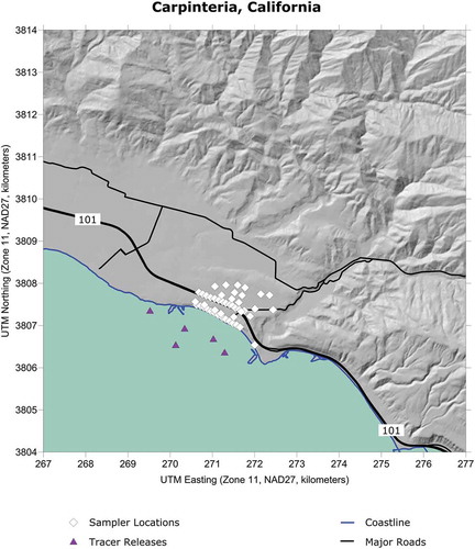
The four model evaluation data sets used in the current study were provided by EPA Region 10 from the archives supporting development of CALPUFF for BOEM (Earth Tech, 2006) and used to assess OCD version 4 (DiCristofaro and Hanna, 1989). Characteristics for the studies are listed in Table 1. These studies include hours with a wide range of overwater atmospheric stabilities based on the range of air-sea temperature differences and wind speeds. The tracer measurements in Pismo Beach (Figure 1) and Cameron (Figure 2) occur in level terrain near the shoreline downwind of offshore tracer releases. These two studies provide tests of overwater dispersion without the complications due to air modification over the land or complex terrain. The Ventura (Figure 3) study is similar; however, the receptors are located 500–1000 m inland from the shoreline, so some air modification may have affected dispersion in this study. The Carpinteria (Figure 4) complex terrain tracer study involved shoreline measurements observed on a 30-m bluff near plume level. The Carpinteria data set had much lighter winds, and the transport distances were less than the other three studies. The Carpinteria study also had tracer releases designed to assess shoreline fumigation. These hours were excluded from the model evaluation.

Table 1. Overwater tracer study characteristics.

Location	Period	Number of Samples	Structure, Release Height Above the Water (m)	Transport^a Distance (km)	Wind Speeds^b (m sec^−1)	Air-Sea^c Temperature Differences (°C)
Pismo Beach, CA	December 1981	15	Boat, 13.1	6.4 to 8.3	1.6 to 10.9	−0.8 to 3.4
Pismo Beach, CA	June 1982	16	Boat, 13.6	6.1 to 6.7	2.7 to 12.7	0.6 to 3.7
Cameron, LA	July 1981	9	Platform, 13	7.0 to 10.0	2.1 to 5.1	−4.5 to −1.2
Cameron, LA	February 1982	17	Platform and Boat, 13	4.5 to 7.8	3.3 to 6.2	−0.8 to 5.0
Carpinteria, CA	September 1981	27	Boat, 18.3 to 60	0.8 to 1.5	1.0 to 5.4	−1.1 to 2.8
Ventura, CA	September 1980	9	Boat, 8.1	6.9 to 10.8	4.1 to 6.9	−2.1 to 0.0
Ventura, CA	January 1981	8	Boat, 8.1	6.9 to 8.0	4.0 to 5.8	−0.9 to 1.8

^aDistance from release point to receptor with the highest measured concentration.

^bWind speed measurement heights: Pismo at 20.5 m; Cameron at 10–18 m; Carpinteria at 24–49 m; and Ventura at 20.5 m.

^cTemperature and humidity measurement heights: Pismo at 7 m; Cameron at 10–18 m; Carpinteria at 9 m; and Ventura at 7 m.

Figure 1. Pismo Beach field study release points and monitoring locations.

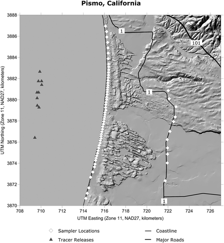
Figure 2. Cameron field study release points and monitoring locations.

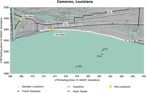
Figure 3. Ventura field study release points and monitoring locations.

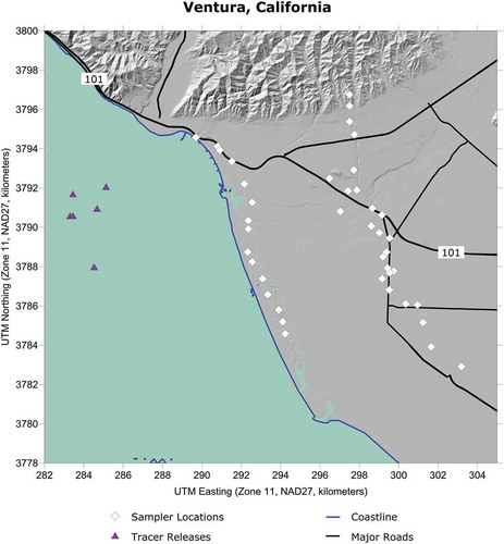
Figure 4. Carpinteria field study release points and monitoring locations.

In order to compare the performance of AERCOARE-AERMOD versus CALPUFF and OCD, the same general data sets were used for the model evaluation. The overwater meteorological data input files processed by AERCOARE were the same with a few exceptions:

• Reported mixing heights were used as an estimate for the convective mixing height for AERMOD during unstable hours. Several options for the mechanical mixing were tested, including using the mixing height reported in the studies and an alternate estimate for the mechanical mixing height based on eq 34.

• The overwater data for OCD and CALPUFF from the field studies contain both temperature lapse rate above the water and air-sea temperature difference measured using different methods. In several instances, the air-sea temperature difference observations suggested slightly unstable or neutral conditions, whereas the lapse rate measurements were characteristic of a very stable surface layer (e.g., 0.06 °C m⁻¹). We assumed the lapse rate was more indicative of the surface layer structure and adjusted the reported air-sea temperature difference to be at least as stable as indicated by the lapse rate. Note: OCD and CALPUFF allow the overwater lapse rate variable to trigger extremely stable conditions irrespective of all other variables, including the air-sea temperature difference.

In past evaluation studies for CALPUFF and OCD, maximum model predictions were compared with the highest measured observations for each hour. For the Pismo Beach, Cameron, and Ventura near-level terrain data sets, this was accomplished by simply ensuring the wind direction used in the simulations caused the plume centerline to pass over the receptor with the highest measured concentrations.

In complex terrain the highest ground level concentrations can occur off the plume centerline. The Carpinteria complex terrain data set was simulated using measured wind directions to consider the effects of terrain elevation on the model predictions.

Model performance measures

Statistical procedures were applied to evaluate model performance using the Pismo Beach, Cameron, Ventura, and Carpinteria overwater tracer studies and to assess whether the AERCOARE-AERMOD modeling approach was biased towards underestimates. Model bias towards underprediction would typically not be acceptable for a regulatory modeling approach. In addition, the procedures were applied to examine which of the five cases for preparing the meteorological data performed statistically better within a regulatory modeling framework. The procedures are designed to evaluate how well the modeling approach explains the frequency distribution of the observed concentrations, especially the upper-end or highest observed concentrations. The analysis also measures the model’s ability to explain the temporal variability of the observations. Given two unbiased models, the approach with the least amount of scatter would generally be preferred.

The statistical methods and measures are similar to the techniques applied in the EPA evaluation of AERMOD (EPA, 2003) as are discussed below:

Quantile-quantile (Q-Q) plots were prepared to test the ability of the model predictions to represent the frequency distribution of the observations. Q-Q plots are simple ranked samples of predicted and observed concentrations unpaired in time, such that any rank of the predicted concentration is plotted against the same ranking of the observed concentration. The Q-Q plots can be inspected to examine whether the predictions are biased towards underestimates at the important upper end of the frequency distribution.

The robust highest concentration (RHC) has been used in most EPA model evaluation studies to measure the model’s ability to characterize the upper end of the frequency distribution. Note this can also be accomplished by visual inspection of the Q-Q plots. Recent ambient air quality standards are no longer based on the maximum concentration, so the RHC as statistical measure is somewhat less relevant than in past studies. The RHC (µ sec m⁻³) is calculated from

(37)

where c_n is the nth highest concentration (µ sec m⁻³) and is the average of the (n − 1) highest concentrations (µ sec m⁻³). Concentrations in eq 37 and for all statistical measures were normalized by the tracer release rate, hence the units of µ sec m⁻³. For the small-sample-size data sets in the current analysis, n was taken to be 10, less than the value of 26 used in many EPA model evaluation studies.

Tables of statistical measures were prepared using the BOOT (Level 2/2/2007) statistical model evaluation package (Chang and Hanna, 2005). The BOOT program is an update of the package applied in the CALPUFF evaluation (Earth Tech, 2006).

The BOOT program was applied to provide information regarding bias of the mean, scatter or precision, and confidence limits using the bootstrap resampling method. The statistics were performed using the natural logarithm of the predictions and observations. Such geometric methods are more appropriate than linear statistics when the data exhibit a log-normal distribution and/or vary over several orders of magnitude. Bias of the geometric mean (MG) is measured from

(38)

where c_o and c_p are the observed and predicted concentrations, respectively. MG is a symmetric measure independent of the magnitude of the concentration where for a perfect model, MG = 1 and a factor of 2 is bounded by 0.5 < MG < 2. Note there are no zero observed or predicted concentrations in the evaluation data set. The scatter or precision is measured with the geometric variance (VG):

(39)

VG is similar to the normalized mean square error in linear statistics and measures scatter about a 1:1 observation-to-prediction ratio. A random scatter of a factor of 2 is equivalent to VG = 1.6, and VG = 12 would indicate a random scatter equivalent to a factor-of-5 bias.

The BOOT program also provides other descriptive statistics, including the geometric correlation coefficient and the fraction within a factor of 2. Importantly, bootstrap resampling methods are used by BOOT to test whether differences in MG or VG between the different cases are statistically significant.

Results and discussion

This section summarizes the results of the model performance evaluation. The statistical measures and data sets described above were applied to evaluate several options for the application of AERCOARE-AERMOD, low-wind-speed options for AERMOD, and AERCOARE-AERMOD compared with OCD and CALPUFF. For OCD and CALPUFF, the predictions are taken from the BOEM model evaluation study (Earth Tech, 2006). A supplemental spreadsheet accompanies this paper with the observations, various model predictions, and overwater meteorological observations used in our study.

Performance for AERCOARE-AERMOD options

Environ (2012a) evaluated AERCOARE-AERMOD options using the techniques and data discussed above. We have updated the supporting simulations from Environ (2012a) with AERMOD version 15181 (EPA, 2015) using the meteorological data sets prepared for each of the four field studies. As in Environ (2012a), five cases were considered using various combinations of the many possible methods to assemble the data. Four cases examined model performance for different AERCOARE options, and the fifth case tested an alternative expression for horizontal dispersion. Descriptions of the five cases are as follows:

• Case 1: Require Abs(L) > 5, use σ_θ measurements, and use the Venkatram equation for z_im and require z_im > 25 m.

• Case 2: Require Abs(L) > 5, use AERMOD-predicted σ_θ, and use the Venkatram equation for z_im and require z_im > 25 m.

• Case 3: Require Abs(L) > 1, use σ_θ measurements, and use observed mixing heights for the mechanical mixing height (z_im).

• Case 4: Require Abs(L) > 5, use σ_θ measurements, and use observed mixing heights for the mechanical mixing height (z_im).

• Case 5: Require Abs(L) > 5, use σ_θ measurements, use the Venkatram equation for z_im and require z_im > 25 m, and modify AERMOD to use the Draxler equation for the ambient lateral dispersion parameter (Draxler, 1976):

  (40)
  This equation is used by OCD and is the default for CALPUFF.

Case 5 was included to assess the sensitivity of the lateral dispersion term in AERMOD to the mixing height. The BOEM CALPUFF evaluations found this equation performed better than several alternatives similar to the formulation used by AERMOD (Earth Tech, 2006).

AERCOARE-AERMOD simulations were conducted to predict concentrations from the Pismo Beach, Cameron, Ventura, and Carpinteria field studies using four different methods for the preparation of the meteorological data, and for Case 5, the differences caused by an alternative lateral dispersion term. AERMOD version 15181 was applied using default dispersion options for rural flat terrain for the Pismo Beach, Ventura, and Cameron simulations. Complex terrain was assumed for the Carpinteria data set. Peak predicted concentrations were compared with peak observed concentrations, resulting in a total of 101 paired-in-time samples for statistical analysis with the techniques described above. In order to be independent of the tracer emission rate, the simulations were performed with a unit emission rate of 1 g sec⁻¹ and the observations were normalized by the tracer release rate providing concentrations in units of µ sec m⁻³.

Q-Q plots comparing the five different AERCOARE-AERMOD options for the four field studies are shown in Figure 5. The five AERCOARE-AERMOD simulations generally predict the frequency distribution within a factor of 2. The predictions tend to be biased towards overprediction for the highest concentrations and underprediction for the lower end of the frequency distribution. This tendency is most apparent for the Pismo Beach data set. Generally, higher concentrations are overpredicted using the AERMOD σ_θ estimates (Case 2). Important for regulatory applications, AERCOARE-AERMOD does not appear to be biased towards underestimates for the higher end of the frequency distribution, regardless of the options examined in this study.

Figure 5. Q-Q plots of AERCOARE-AERMOD predictions versus observations for (a) Cameron, (b) Carpinteria, (c) Pismo Beach, and (d) Ventura.

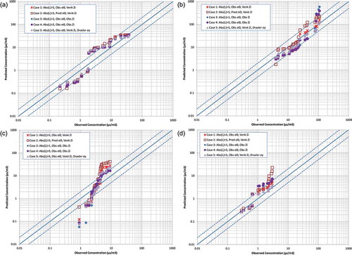
The BOOT program statistics and the RHC for each data set and AERCOARE-AERMOD option are summarized in Table 2. The full BOOT program output from the current application of AERMOD version 15181 are similar to the results presented in Environ (2012a) and will not be presented here. For all the data sets and especially the Pismo Beach data set, the predicted concentrations are more variable than the observations based on comparison of the geometric standard deviations. The Pismo Beach field study had the poorest paired-in-time model performance, and the RHC is significantly overpredicted by each modeling alternative. Overall, the performance statistics tend to be the best for Case 5 with the modified lateral dispersion estimates. Case 5 tended to have the highest geometric correlation coefficients, highest percentage within a factor of 2, and lowest scatter (VG).

Table 2. AERCOARE-AERMOD model options performance.

Data Set	Case	Description	Geometric Mean (µ sec m^−3)	Geometric SD	MG	VG	Geometric Correlation	Factor of 2	RHC (µ sec m^−3)
All data (101 samples)	0	Observations	4.5	1.36	1.00	1.00	1.00	1.00	125
	1	Abs(L) > 5, Obs σθ, Venk zi	4.7	1.60	0.96	3.21	0.75	0.54	146
	2	Abs(L) > 5, Pred σθ, Venk zi	6.8	1.73	0.67	4.93	0.72	0.47	311
	3	Abs(L) > 1, Obs σθ, Obs zi	4.7	1.67	0.97	4.05	0.71	0.48	493
	4	Abs(L) > 5, Obs σθ, Obs zi	4.9	1.57	0.93	3.23	0.74	0.47	333
	5	Abs(L) > 5, Obs σθ, Venk zi, Draxler σy	4.6	1.53	0.99	2.60	0.78	0.55	116
Ventura, CA (flat, 17 samples)	0	Observations	1.2	0.76	1.00	1.00	1.00	1.00	4
	1	Abs(L) > 5, Obs σθ, Venk zi	1.6	1.03	0.73	1.81	0.73	0.77	6
	2	Abs(L) > 5, Pred σθ, Venk zi	2.4	1.37	0.50	5.28	0.62	0.59	20
	3	Abs(L) > 1, Obs σθ, Obs zi	2.1	1.18	0.57	2.58	0.75	0.59	8
	4	Abs(L) > 5, Obs σθ, Obs zi	2.1	1.18	0.57	2.58	0.75	0.59	8
	5	Abs(L) > 5, Obs σθ, Venk zi, Draxler σy	1.4	0.88	0.87	1.41	0.77	0.94	4
Pismo Beach, CA (flat, 31 samples)	0	Observations	3.5	0.50	1.00	1.00	1.00	1.00	9
	1	Abs(L) > 5, Obs σθ, Venk zi	3.7	1.39	0.93	6.17	0.27	0.45	35
	2	Abs(L) > 5, Pred σθ, Venk zi	5.9	1.45	0.59	12.90	0.04	0.26	54
	3	Abs(L) > 1, Obs σθ, Obs zi	3.2	1.40	1.09	7.53	0.14	0.45	18
	4	Abs(L) > 5, Obs σθ, Obs zi	3.8	1.23	0.91	4.30	0.26	0.45	20
	5	Abs(L) > 5, Obs σθ, Venk zi, Draxler σy	3.3	1.33	1.04	4.81	0.35	0.42	31
Cameron, LA (flat, 26 samples)	0	Observations	3.2	1.41	1.00	1.00	1.00	1.00	41
	1	Abs(L) > 5, Obs σθ, Venk zi	4.1	1.84	0.78	3.03	0.83	0.42	50
	2	Abs(L) > 5, Pred σθ, Venk zi	4.2	1.87	0.76	3.60	0.81	0.42	52
	3	Abs(L) > 1, Obs σθ, Obs zi	3.7	1.77	0.86	2.67	0.83	0.46	40
	4	Abs(L) > 5, Obs σθ, Obs zi	3.7	1.79	0.84	2.68	0.84	0.46	44
	5	Abs(L) > 5, Obs σθ, Venk zi, Draxler σy	4.1	1.70	0.76	2.56	0.84	0.46	41
Carpinteria, CA (complex, 27 samples)	0	Observations	20.1	0.93	1.00	1.00	1.00	1.00	143
	1	Abs(L) > 5, Obs σθ, Venk zi	14.0	1.19	1.44	2.29	0.72	0.59	186
	2	Abs(L) > 5, Pred σθ, Venk zi	24.3	1.29	0.83	2.10	0.76	0.67	334
	3	Abs(L) > 1, Obs σθ, Obs zi	15.0	1.50	1.34	3.95	0.66	0.44	506
	4	Abs(L) > 5, Obs σθ, Obs zi	14.2	1.36	1.42	3.19	0.67	0.41	341
	5	Abs(L) > 5, Obs σθ, Venk zi, Draxler σy	15.5	0.97	1.30	1.90	0.69	0.56	133

Comparing the AERCOARE-AERMOD options, there is no clear choice for the best method to prepare the meteorological data. Case 2 using the AERMOD σ_θ estimates seems to result in overprediction for the combined data set and each individual data set. Depending on the data set, the method used to estimate the mechanical mixing height influenced the results. The observed mixing height seemed to perform the best for Pismo Beach, whereas the Venkatram (eq 34) estimate worked the best overall. Allowing the Monin-Obukhov length to become very stable (Case 3) also resulted in severe overpredictions, as shown in Figure 5c and 5d for Pismo Beach and Ventura, respectively. Removing the dependency of the lateral dispersion term on mixing height (Case 5) also improved model performance in some instances, especially as shown in Figure 5b for the Carpinteria data set where observed mixing heights appear to be the most uncertain. Further discussions of model performance by study area and AERCOARE-AERMOD option can be found in Environ (2012a).

Figure 6a shows a Q-Q plot comparing different minimum mixing height assumptions for the Carpinteria field study. Light winds and stable conditions resulted in very low predicted mixing heights and high concentrations for several hours. For the Carpinteria field study, the AERCOARE-predicted friction velocities during several hours are less than 0.005 m sec⁻¹, resulting in mechanical mixing heights less than 1 m. Out of the 36 hr of data, 50% of the mixing heights are predicted to be less than 25 m for the light winds observed during this study. Very high predictions result from allowing the mixing height to be as low as 1 m, and better model performance was found by requiring the mixing height be at least 25 m. As shown in Figure 5b, such overprediction could also be avoided by replacing the AERMOD horizontal dispersion parameter by a simpler expression as in Case 5.

Figure 6. Q-Q Plots of AERCOARE-AERMOD: (a) sensitivity to minimum mixing height at Carpinteria; (b) low-wind options with σ_θ data at Carpinteria; (c) low-wind options without σ_θ data at Carpinteria; and (d) low-wind options without σ_θ data at Pismo Beach.

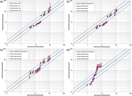
AERMOD version 15181 includes three low-wind dispersion options designed to reduce the tendency towards overprediction during light wind stable conditions. Figures 6b–d compare the three low-wind options for two field studies where such conditions resulted in higher predictions. The corresponding statistics from the BOOT program are shown in Table 3. The Q-Q plot in Figure 6b compares the three low-wind options with the EPA default option for the Carpinteria data set. For the Case 1 set of AERCOARE-AERMOD options, σ_θ data were provided to AERMOD and the low-wind options only slightly affected the AERMOD predictions. However, when observed σ_θ data were withheld from AERMOD as in the Case 2 simulations, the low-wind options reduced the degree of overprediction for Carpinteria (Figure 6c) and for Pismo Beach (Figure 6d). The statistics in Table 3 also suggest improved model performance for most of the measures when the low-wind options are employed in the absence of observed σ_θ data. We would recommend using σ_θ measurements when available and one of the low-wind options in the absence of such data. Comparisons with the measurements from the tracer studies did not provide enough information for the recommendation of a preferred low-wind option.

Table 3. AERCOARE-AERMOD low-wind-speed option model performance.

Data Set	Description	Geometric Mean (µ sec m^−3)	Geometric SD	MG	VG	Geometric Correlation	Factor of 2	RHC (µ sec m^−3)
Carpinteria, CA (complex, 27 samples)	Observations	20.1	0.93	1.00	1.00	1.00	1.00	143
	AERCOARE-AERMOD (Case 1)	14.0	1.19	1.44	2.29	0.72	0.59	186
	As above with LOWWIND 1 Option	14.6	1.26	1.38	2.27	0.74	0.48	222
	As above with LOWWIND 2 Option	13.7	1.19	1.47	2.30	0.72	0.56	181
	As above with LOWWIND 3 Option	12.1	1.12	1.67	2.57	0.69	0.44	141
Carpinteria, CA (complex, 27 samples)	Observations	20.1	0.93	1.00	1.00	1.00	1.00	143
	AERCOARE-AERMOD (Case 2)	24.3	1.29	0.83	2.10	0.76	0.67	334
	As above with LOWWIND 1 Option	16.6	1.19	1.22	1.94	0.75	0.44	213
	As above with LOWWIND 2 Option	19.9	1.10	1.01	1.72	0.75	0.67	190
	As above with LOWWIND 3 Option	18.5	1.04	1.09	1.72	0.73	0.67	154
Pismo Beach, CA (flat, 31 samples)	Observations	3.5	0.50	1.00	1.00	1.00	1.00	9
	AERCOARE-AERMOD (Case 2)	5.9	1.45	0.59	12.90	0.04	0.26	54
	As above with LOWWIND 1 Option	4.3	1.24	0.80	5.98	0.05	0.32	32
	As above with LOWWIND 2 Option	5.1	1.31	0.68	7.90	0.03	0.29	36
	As above with LOWWIND 3 Option	5.0	1.29	0.70	7.46	0.02	0.29	33

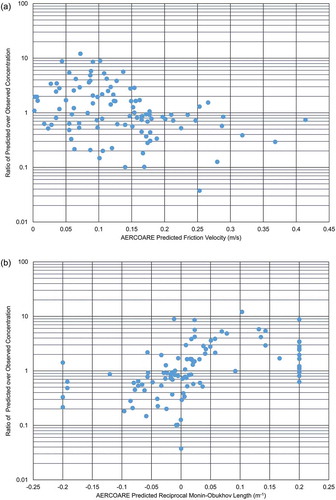
As shown in Figure 5 and Figure 6, AERCOARE-AERMOD had a tendency to overpredict the higher observations and underpredict the lower range of the frequency distribution. Figure 7 shows Case 1 predicted over observed concentration ratios versus the friction velocity (u_*) and against stability characterized by the reciprocal Monin-Obukhov length (1/L) using paired samples from the four tracer studies. AERCOARE-AERMOD had a slight tendency to underpredict (c_p/c_o < 1) with increasing wind speed, as is shown in Figure 7a. Figure 7b suggests that the combined AERCOARE-AERMOD predictions tended to be biased toward overprediction for stable conditions (1/L > 0) and towards underprediction for unstable conditions (1/L < 0). The tendencies tend to explain the behavior exhibited in the Q-Q plots shown in Figure 5 and Figure 6, since the higher concentrations were associated with stable conditions in the four tracer studies.

Figure 7. AERCOARE-AERMOD (Case 1) predicted to observed concentration ratios: (a) versus friction velocity and (b) versus reciprocal Monin-Obukhov length.

AERCOARE-AERMOD comparisons with OCD and CALPUFF

Predictions from OCD and CALPUFF for the four field studies were extracted from the BOEM archives (Earth Tech, 2006) and used for comparisons with AERCOARE-AERMOD. The BOEM study evaluated several options for CALPUFF and OCD, and the best performing options found by the study authors were selected for comparison with AERCOARE-AERMOD. Namely, the model performance comparisons used the following:

• CALPUFF Option B. Option B used observed σ_θ measurements, horizontal dispersion from the Draxler equation (eq 40; Draxler, 1976), and default COARE options. The predictions are based on CALPUFF version 5.751. Note: We have verified the original version 5.751 simulations are not significantly different the simulations with a more recent CALPUFF regulatory version 5.8.4.

• OCD observed σ_θ. These predictions were also taken from the BOEM study. The predictions are based on OCD version 5 using observed σ_θ measurements.

• AERCOARE-AERMOD Case 1. Require Abs(L) > 5, use σ_θ measurements, use the Venkatram equation for z_im and require z_im > 25 m. Based on the model performance statistics presented above, this set of options provided the best model performance not involving the modification to the AERMOD code (as in Case 5).

Earth Tech (2006) provides further details concerning the application of OCD and CALPUFF. The same overwater input meteorological data and release characteristics were used for all three models: AERCOARE-AERMOD, OCD, and CALPUFF.

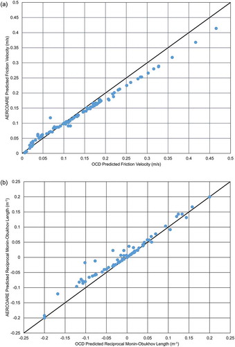
The coupled AERCOARE-AERMOD modeling approach involves the AERCOARE characterization of air-sea energy fluxes and atmospheric stability combined with the AERMOD dispersion component. In order to understand the performance of the coupled system, the predictions from AERCOARE were first compared with OCD’s predictions for the friction velocity (u_*) and the atmospheric stability as characterized by the reciprocal of the Monin-Obukhov length (1/L). These variables heavily influence the dispersion predictions of both AERMOD and OCD.

Figure 8 displays a comparison of AERCOARE- and OCD-predicted u_* and 1/L given the same overwater measurements from the four field studies. AERCOARE-predicted friction velocities in Figure 8a are very similar to the OCD predictions, with slightly lower estimates for higher winds and higher estimates for lighter winds. Atmospheric stability predictions shown in Figure 8b are also similar. For stable conditions (1/L > 0), the estimates from OCD and AERCOARE are very close to each other. For unstable conditions, the AERCOARE estimates are somewhat less unstable, but generally follow the OCD predictions. CALPUFF includes the same COARE 3.0 algorithms as AERCOARE, so the results presented in Figure 8 suggest that differences in model performance discussed below are due to the dispersion modules or possibly the characterization of the mixing height.

Figure 8. Comparison of AERCOARE- versus OCD-predicted (a) friction velocity and (b) reciprocal Monin-Obukhov length.

Q-Q plots constructed from predictions of the three models and observations from the four field studies are shown in Figure 9. All three models explained the frequency distribution of the observations within a factor of 2 for the Cameron, Carpinteria, and Ventura data sets. The upper ends of the frequency distributions are clustered together, and when applied for regulatory purposes, AERMOD-AERCOARE would tend to predict maximum concentrations similar to or a little higher than OCD or CALPUFF. CALPUFF tended to have the best performance for Pismo Beach, whereas both OCD and AERCOARE-AERMOD underpredicted the lower observed concentrations range, and AERCOARE-AERMOD overpredicted the higher observed concentrations. As shown in Figure 5c, AERCOARE-AERMOD predictions were improved for Pismo Beach when a simpler expression for the horizontal dispersion parameter independent of the mixing height was used instead of eq 35 used by AERMOD. Another possibility might be the Venkatram equation, even with a lower limit of 25 m, underpredicted the mixing height for many of the stable hours with the higher predictions.

Figure 9. Q-Q plots of AERCOARE-AERMOD, OCD, and CALPUFF predictions versus observations for (a) Cameron, (b) Carpinteria, (c) Pismo Beach, and (d) Ventura.

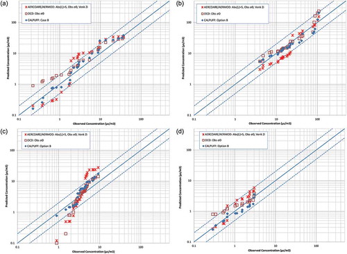
The BOOT program statistics and the RHC for each data set and model are summarized in Table 4. Model performance varied by data set and statistical measure, but was similar for the combined data set, Ventura, Cameron, and Carpinteria. In most instances, the performance measures are not different in a statistical sense. However, the AERCOARE-AERMOD prediction scatter (high VG and low geometric correlation coefficient) was higher for the Pismo Beach study and the four data sets overall. Output from the BOOT programs suggests that the difference is significant at the 95% confidence limit for Pismo Beach. As the COARE algorithm is included in both AERCOARE and CALPUFF and is similar to the internal methods used by OCD (Figure 8), the differences are likely due to the different dispersion methodologies and not the predictions of the air-sea energy fluxes.

Table 4. AERCOARE-AERMOD, CALPUFF, and OCD model performance.

Data Set	Description	Geometric Mean (µ sec m^−3)	Geometric SD	MG	VG	Geometric Correlation	Factor of 2	RHC (µ sec m^−3)
All Data (101 samples)	Observations	4.5	1.36	1.00	1.00	1.00	1.00	125
	AERCOARE-AERMOD (Case 1)	4.7	1.60	0.96	3.21	0.75	0.54	146
	OCD (Obs. IY)	5.4	1.36	0.84	2.09	0.81	0.56	211
	CALPUFF (Option B)	4.7	1.44	0.97	1.89	0.84	0.58	141
Ventura, CA (flat, 17 samples)	Observations	1.2	0.76	1.00	1.00	1.00	1.00	4.3
	AERCOARE-AERMOD (Case 1)	1.6	1.03	0.73	1.81	0.73	0.77	6.3
	OCD (Obs. IY)	1.6	0.44	0.75	1.72	0.47	0.65	3.6
	CALPUFF (Option B)	1.0	0.68	1.22	1.43	0.70	0.71	3.3
Pismo Beach, CA (flat, 31 samples)	Observations	3.5	0.50	1.00	1.00	1.00	1.00	9
	AERCOARE-AERMOD (Case 1)	3.7	1.39	0.93	6.17	0.27	0.45	35
	OCD (Obs. IY)	3.2	1.12	1.09	2.69	0.47	0.58	16
	CALPUFF (Option B)	4.1	0.83	0.85	1.77	0.47	0.52	17
Cameron, LA (flat, 26 samples)	Observations	3.2	1.41	1.00	1.00	1.00	1.00	41
	AERCOARE-AERMOD (Case 1)	4.1	1.84	0.78	3.03	0.83	0.42	50
	OCD (Obs. IY)	5.2	1.11	0.61	1.96	0.89	0.58	47
	CALPUFF (Option B)	3.7	1.59	0.85	2.78	0.78	0.54	51
Carpinteria, CA (complex, 27 samples)	Observations	20.1	0.93	1.00	1.00	1.00	1.00	143
	AERCOARE-AERMOD (Case 1)	14.0	1.19	1.44	2.29	0.72	0.59	186
	OCD (Obs. IY)	22.0	0.99	0.92	1.88	0.66	0.48	218
	CALPUFF (Option B)	18.4	0.87	1.09	1.68	0.69	0.63	143

Summary

This study was initiated to examine whether the AERCOARE overwater meteorological preprocessor combined with the EPA overland dispersion model AERMOD could be used as an alternative to OCD the current EPA regulatory offshore model. The overland meteorological preprocessor for AERMOD (AERMET) does not contain routines to characterize energy fluxes in the marine boundary layer. AERCOARE includes algorithms to predict surface energy fluxes and stability from routine overwater measurements using the COARE bulk parameterization method often used in studies of the marine boundary layer. AERCOARE allows the regulatory and source type flexibilities built into AERMOD for overland industrial sources to be applied to offshore sources.

The COARE algorithm in AERCOARE estimates the energy fluxes over water using empirical relationships based on the differences in wind speed, temperature, and relative humidity in the air to the conditions at the surface. Conditions at the surface of the ocean are parameterized using the surface temperature– and wind speed–dependent surface roughness lengths for momentum, heat, and moisture. Optional techniques are included to account for the difference between the skin or sea surface temperature and the temperature measured at depth below the surface.

Model performance for the combined AERCOARE-AERMOD modeling approach was evaluated against tracer measurements from four overwater field studies: Cameron, Louisiana; Carpinteria, California; Pismo Beach, California; and Ventura, California. These same tracer studies were used as the basis for development of OCD and more recently to evaluate overwater routines incorporated into CALPUFF. CALPUFF also includes the COARE algorithms to predict overwater surface energy fluxes.

Relatively better AERCOARE-AERMOD model performance was found when lateral turbulence measurements were available and when several key input variables to AERMOD were constrained. Namely, requiring the mixed layer height to be at least 25 m and not allowing the absolute value of the Monin-Obukhov length to be less than 5 m, compared with AERMOD’s constraint of 1 m, improved model performance in low-wind-speed stable conditions. Options for low-wind-speed dispersion in AERMOD also affected and improved the model performance results, especially when lateral turbulence data were not available or were withheld from the simulations.

Observed frequency distributions from three of the four field studies were generally predicted within a factor of 2 throughout the range of observed concentrations. Important from a regulatory perspective, AERCOARE-AERMOD did not underpredict the higher end of the observed frequency distribution. For Pismo Beach, AERCOARE-AERMOD significantly overpredicted the higher observations and underpredicted the lower observations. The modeling approach had tendency to overpredict concentrations under stable conditions and underpredict concentrations of unstable conditions. Model performance was improved when a simpler expression for the horizontal dispersion parameter, σ_y, was incorporated into AERMOD. The current formulation in AERMOD depends on the mixed layer height, a variable both difficult to predict and derive from measurements.

The model performance for the combined AERCOARE-AERMOD modeling approach was found to be comparable to OCD and CALPUFF for the same tracer studies. AERCOARE-predicted fluxes and stabilities were similar to those predicted by OCD, so differences in model performance can be attributed to the AERMOD dispersion component. Many model performance measures were found to be similar, but CALPUFF and to a lesser extent OCD had significantly less scatter and better performance for the Pismo Beach tracer study.

AERCOARE-AERMOD could be applied as an alternative to the current EPA model OCD for many regulatory applications using the same basic overwater meteorological data. This approach would allow AERMOD methods for plume impingement on elevated terrain, building downwash, nitrogen oxides to nitrogen dioxide (NO₂) conversion, design concentration calculations, area sources, volume sources, buoyant line sources, hourly variable emissions, and many other features to be used for offshore sources. Shoreline fumigation and platform downwash modules are not included in AERMOD, and there may be instances where OCD and/or CALPUFF are more appropriate when such issues are thought be important to the application.

Acknowledgment

The authors wish to thank Dr. Ronald Lai and Mr. Dirk Herkhoff of the Bureau of Ocean Energy Management, Department of the Interior, for their proactive efforts to advance the science of overwater model dispersion models for regulatory application and the collaboration with the U.S. Environmental Protection Agency, Region 10. In addition, we would like to thank Dr. Chris Fairall, National Oceanic and Atmospheric Administration Earth System Research Laboratory, Physical Science Division, Boulder, Colorado, for the COARE 3.0 FORTRAN code, advice on the application of COARE 3.0, and his many years of research in the development of bulk parametrization for estimating air-seas energy fluxes.

Funding

The studies associated with this work were funded by the U.S. Department of the Interior, Bureau of Ocean Energy Management, Environmental Studies Program, Washington, D.C., and the U.S. Environmental Protection Agency, Region 10, Seattle, Washington.

Supplemental data for this article can be accessed on the publisher’s website.

Additional information

Funding

The studies associated with this work were funded by the U.S. Department of the Interior, Bureau of Ocean Energy Management, Environmental Studies Program, Washington, D.C., and the U.S. Environmental Protection Agency, Region 10, Seattle, Washington.

Notes on contributors

Herman Wong

Herman Wong is a regional atmospheric scientist/air quality modeler with the U.S. Environmental Protection Agency Region 10 in Seattle, Washington.

Rob Elleman

Rob Elleman is a meteorologist with the U.S. Environmental Protection Agency Region 10 in Seattle, Washington.

Eric Wolvovsky

Eric Wolvovsky is a meteorologist with the Department of the Interior, Bureau of Ocean Energy Management, Sterling, Virginia.

Ken Richmond

Ken Richmond is Senior Manager, Air Quality Modeling, for Ramboll Environ at Lynnwood, Washington.

James Paumier

James Paumier is a project manager for Amec Foster Wheeler Environment & Infrastructure, Inc. in Durham, North Carolina.

References

- Arya, S.P. 1988. Introduction to Micrometeorology. San Diego, CA: Academic Press.
- Brunke, M.A., C.W. Fairall, X. Zeng, L. Eymard, and J.A. Curry.. 2003. Which bulk aerodynamic algorithms are least problematic in computing ocean surface turbulent fluxes? J. Climate 16: 619–635. doi:10.1175/1520-0442(2003)016%3C0619:WBAAAL%3E2.0.CO;2
- Cimorelli, A.J., S.G. Perry, A. Venkatram, J.C. Weil, R.J. Paine, R.B. Wilson, R.F. Lee, W.D. Oetres, and R.W. Brode. 2005. AERMOD: A dispersion model for industrial source applications. Part I: General model formulation and boundary layer characterization. J. Appl. Meteorol. 44:682–693. doi:10.1175/JAM2227.1
- Chang, J.C., and K.J. Hahn. 1997. User’s Guide for the Offshore and Coastal Dispersion (OCD) Model Version 5. MMS Contract No. 1435-96-PO-51307, November 1997. http://www.epa.gov/ttn/scram/dispersion_prefrec.htm#ocd (accessed December 15, 2008)
- Chang, J.C., and S.R. Hanna. 2005. Technical Descriptions and User’s Guide for the BOOT Statistical Model Evaluation Software Package, Version 2.0. July 10, 2005. http://www.harmo.org/Kit/Download.asp (accessed June 9, 2015)
- DiCristofaro, D.C., and S.R. Hanna. 1989. OCD The Offshore and Coastal Dispersion Model, Version 4, Volume I: User’s Guide. MMS Contract No. 14-12-001-30396, November 1989. Herndon, VA: Minerals Management Service, U.S. Department of the Interior.
- Draxler, R.R. 1976. Determination of atmospheric diffusion parameters. Atmos. Environ. 10:99–105. doi:10.1016/0004-6981(76)90226-2
- Earth Tech. 2006. Development of the Next Generation of Air Quality Models for the Outer Continental Shelf (OCS) Applications, Final Report: Volume 1. Prepared for Minerals Management Service, U.S. Department of Interior, Herndon, VA. Contract 1435-01-01-CT-31071, March 2006.
- Environ. 2012a. Evaluation of the Combined AERCOARE/AERMOD Modeling Approach for Offshore Sources. Prepared for U.S. Environmental Protection Agency Region 10, Seattle, WA. EPA Contract EP-D-08-102, Work Assignment 5-17, EPA 910-R-12-007, October 2012.
- Environ. 2012b. Draft User’s Manual: AERCOARE Version 1.0. Prepared for U.S. Environmental Protection Agency Region 10, Seattle, WA. EPA Contract EP-D-08-102, Work Assignment 5-17, EPA 910-R-12-008, October 2012.
- Fairall, C.W., and E.F. Bradley. 2003. The TOGA-COARE Air-Sea Flux Algorithm. Boulder, CO: National Oceanic and Atmospheric Administration/Environmental Research Laboratories/Environmental Technology Laboratory, September 2, 2003. ftp://ftp1.esrl.noaa.gov/users/cfairall/wcrp_wgsf/computer_programs/cor3_0/(accessed September 17, 2015).
- Fairall, C.W., E.F. Bradley, J.S. Godfrey, G.A. Wick, J.B. Edson, and G.S. Young. 1996a. Cool-skin and warm-layer effects on sea surface temperature. J. Geophys. Res. 101:1295–1308. doi:10.1029/95JC03190
- Fairall, C.W., E.F. Bradley, J.E. Hare, A.A. Grachev, and J.B. Edson. 2003. Bulk parameterization of air-sea fluxes: Updates and verification for the COARE Algorithm. J. Climate 16:571–591. doi:10.1175/1520-0442(2003)016<0571:BPOASF>2.0.CO;2
- Fairall, C.W., E.F. Bradley, D.P. Rogers, J.B. Edson, and G.S. Young. 1996b. Bulk parametrization of air-sea fluxes for tropical ocean-global atmosphere coupled-ocean atmosphere response experiment. J. Geophys. Res. 101:3747–3764. doi:10.1029/95JC03205
- Grachev, A.A., and C.W. Fairall. 1997. Dependence of the Monin-Obukhov parameter on the bulk Richardson number of the ocean. J. Appl. Meteorol. 36:406–414. doi:10.1175/1520-0450(1997)036<0406:DOTMOS>2.0.CO;2
- Hanna, S.R., L.L. Schulman, R.J. Paine, J.E. Pleim, and M. Baer. 1985. Development and evaluation of the Offshore and Coastal Dispersion model. J. Air Pollut. Control Assoc. 35:1039–1047. doi:10.1080/00022470.1985.10466003
- Liu, W.T., K.B. Katsaros, and J.A. Businger. 1979. Bulk parameterization of air-sea exchanges of heat and water vapor including molecular constraints at the interface. J. Atmos. Sci. 36:1722–1735. doi:10.1175/1520-0469(1979)036<1722:BPOASE>2.0.CO;2
- Oost, W.A., G.J. Komen, C.M.J. Jacobs, and C. van Oort. 2002. New evidence for a relation between wind stress and wave age from measurements during ASGAMAGE. Bound. Layer Meteorol. 103:409–438. doi:10.1023/A:1014913624535
- Taylor, P.K., and M.A. Yelland. 2001. The dependence of sea surface roughness on the height and steepness of waves. J. Phys. Oceanogr. 31:572–590. doi:10.1175/1520-0485(2001)031<0572:TDOSSR>2.0.CO;2
- U.S. Environmental Protection Agency. 1988. User’s Guide to SDM: A Shoreline Dispersion Model. EPA-450/4-88-016. Research Triangle Park, NC: U.S. Environmental Protection Agency, Office of Air Quality Planning and Standards, September 1988.
- U.S. Environmental Protection Agency. 2003. AERMOD: Latest Features and Evaluation Results. EPA-454/R-03-003. Research Triangle Park, NC: U.S. Environmental Protection Agency, Office of Air Quality Planning and Standards, June 2003.
- U.S. Environmental Protection Agency. 2011a. Memorandum: Model Clearinghouse Review of AERMOD-COARE as an Alternative Model for Application in an Arctic Marine Ice Free Environment. From George Bridgers, EPA Model Clearinghouse director, to Herman Wong, U.S. Environmental Protection Agency regional atmospheric scientist, Office of Environmental Assessment, OEA-095, EPA Region 10, May 6, 2011.
- U.S. Environmental Protection Agency. 2011b. Memorandum: COARE Bulk Flux Algorithm to Generate Hourly Meteorological Data for Use with the AERMOD Dispersion Program; Section 3.2.2.e Alternative Refined Model Demonstration. From Herman Wong, U.S. Environmental Protection Agency Regional Office Modeling Contact to Tyler Fox, Lead Air Quality Modeling Group, Office of Air Quality Planning and Standards, April 1, 2011.
- U.S. Environmental Protection Agency. 2015. Addendum: User’s Guide for the AMS/EPA Regulatory Model—AERMOD ( EPA-454/B-03-001, September 2004). Research Triangle Park, NC: U.S. Environmental Protection Agency, Office of Air Quality Planning and Standards, Air Quality Assessment Division, June 2015.
- Venkatram, A.K. 1980. Estimating the Monin-Obukhov length in the stable boundary layer for dispersion calculations. Bound. Layer Meteorol. 19:481–485. doi:10.1007/BF00122347