Developing particle emission inventories using remote sensing (PEIRS)

ABSTRACT

Information regarding the magnitude and distribution of PM_2.5 emissions is crucial in establishing effective PM regulations and assessing the associated risk to human health and the ecosystem. At present, emission data is obtained from measured or estimated emission factors of various source types. Collecting such information for every known source is costly and time-consuming. For this reason, emission inventories are reported periodically and unknown or smaller sources are often omitted or aggregated at large spatial scale. To address these limitations, we have developed and evaluated a novel method that uses remote sensing data to construct spatially resolved emission inventories for PM_2.5. This approach enables us to account for all sources within a fixed area, which renders source classification unnecessary. We applied this method to predict emissions in the northeastern United States during the period 2002–2013 using high-resolution 1 km × 1 km aerosol optical depth (AOD). Emission estimates moderately agreed with the EPA National Emission Inventory (R² = 0.66–0.71, CV = 17.7–20%). Predicted emissions are found to correlate with land use parameters, suggesting that our method can capture emissions from land-use-related sources. In addition, we distinguished small-scale intra-urban variation in emissions reflecting distribution of metropolitan sources. In essence, this study demonstrates the great potential of remote sensing data to predict particle source emissions cost-effectively.

Implications: We present a novel method, particle emission inventories using remote sensing (PEIRS), using remote sensing data to construct spatially resolved PM_2.5 emission inventories. Both primary emissions and secondary formations are captured and predicted at a high spatial resolution of 1 km × 1 km. Using PEIRS, large and comprehensive data sets can be generated cost-effectively and can inform development of air quality regulations.

View correction statement:

Corrigendum

Introduction

Fine particulate matter (PM_2.5) is a major public health burden associated with a range of adverse health effects (Schwartz and Dockery, 1992; Schwartz, 2001; Pope et al., 2002; Schwartz, Laden, and Zanobetti, 2002; Ren, Williams, and Tong, 2006; Zanobetti and Schwartz, 2006; Turner et al., 2011; Lepeule et al., 2012). As such, identifying particle sources and quantifying their emissions is of paramount importance to the development of air quality standards and the enforcement of emission reduction policies. The U.S. Environmental Protection Agency (EPA) is responsible for developing a nationwide particle emission inventory, the National Emission Inventory (NEI) (EPA, 2008, 2011), which is the most comprehensive database for criteria air pollutants (CAP) and hazardous air pollutants (HAP) emissions. The NEI is updated every 3 years using data collected from state, local, and tribal air agencies and EPA emission trading programs. Collecting information on area and mobile emission sources can be challenging, especially when there are many small sources widely dispersed over a large area. For instance, smaller stationary sources such as wood furnaces and stoves are not defined as major point sources in the NEI and thus are not rigorously regulated. However, these smaller sources may represent a large fraction of the total emissions as bigger industrial sources decrease in intensity due to strict regulations and improved technology. For PM, the current NEI aggregates mobile sources and nonindustrial sources at county level. Information for such broad geographic areas, in combination with measurement error and modeling uncertainties, may limit effectiveness to implement emission regulations. Coarse spatial resolution also limits the utility of the NEI data to assess human health risks or develop air pollution models (EPA, 2008).

Satellite data is increasingly important for air pollution exposure assessment because of scarce and ad hoc spatial–temporal coverage of the federal monitoring network. Satellite data have been incorporated in a variety of air quality applications, including tracking long-term pollution transport, identifying exceptional events such as wildfires, fireworks, and dust storms, and estimating ground-level pollution concentrations (Duncan et al., 2014). Satellite-based sensors have provided information on important air pollutants, such as nitrogen dioxide (NO₂), sulfur dioxide (SO₂), volatile organic compounds (VOCs), and fine particulate matter (PM_2.5) (Martin, 2008). Specifically, a growing number of studies have successfully employed aerosol optical depth (AOD) data to characterize properties and patterns of PM_2.5 (Gupta and Christopher, 2009; Liu, Paciorek, and Koutrakis, 2009; Kloog et al., 2011; Lee et al., 2012; Hu et al., 2014; Kloog et al., 2014).

AOD is a dimensionless measure of the attenuation of light due to the presence of aerosols that prevent light transmission via absorption or scattering. This fundamental property of AOD, with proper correction for absorption and scattering of gases in the atmosphere, makes it a suitable surrogate for the aerosol loading in the atmosphere (Hoff and Christopher, 2009). Nevertheless, vigilant calibration of the AOD data is required due to several physical differences among AOD and ground-level PM_2.5. A critical concern is that AOD represents the total amount of aerosols in the entire atmospheric column while measured PM_2.5 only reflects particles at ground level. The relationship between AOD and PM_2.5 is therefore highly dependent on the vertical distribution of aerosols. Moreover, like all satellite measurements, AOD readings are snapshots of the aerosol distribution at that exact moment, while filter-based PM_2.5 samples are collected over a 24-hr period. This temporal mismatch also influences the association between AOD and ground-level PM_2.5. To address these concerns, multiple techniques including neural network, generalized additive models, and hybrid models have been used to generate AOD-derived PM_2.5 concentrations (Gupta and Christopher, 2009; Lee et al., 2012; Hu et al., 2014; Kloog et al., 2014). Recent advancements in various predictive statistical models (Kloog et al., 2014) have enabled scientists to assess daily PM_2.5 exposures with continuous spatial coverage, which are crucial for legislation development and health effects studies. Nonetheless, satellite data have yet to become a prime resource in predicting particle emissions.

In this study, we introduce a method using satellite AOD data to predict emission inventories for PM_2.5. As a demonstration of the proposed method, we constructed spatially resolved PM_2.5 emission inventories in the U.S. Northeast using 1 km × 1 km daily AOD retrievals during the period of 2002–2013. We derive the emission model based on the concept of one compartment model, which has been applied to the ambient environment in the past to estimate emission fluxes (EPA, 2001), as well as indoor emission sources (Spengler, Samet, and McCarthy, 2001). Our approach has the potential to generate comprehensive emission inventories cost-effectively as compared to the existing ones.

Methods

Data and materials

PM_2.5 ground monitoring concentration data

The study domain is the U.S. Northeast, which includes the states of Connecticut (CT), Massachusetts (MA), Maine (ME), New Hampshire (NH), New York (NY), Rhode Island (RI), and Vermont (VT). We obtained daily averaged PM_2.5 measurements, mostly from integrated filter samples, measured at 124 monitoring sites among those of the U.S. Environmental Protection Agency (EPA) Compliance Network, Air Quality System (AQS), and the Interagency Monitoring of Protected Visual Environments (IMPROVE) database during the period of 2002 to 2013. Daily averaged monitoring PM_2.5 is used to calibrate AOD data into AOD-derived-PM_2.5 concentrations (Figure 1).

Figure 1. Study area and EPA monitoring network.

Satellite aerosol optical depth

The Moderate Resolution Imaging Spectroradiometer (MODIS) instrument on board the Earth Observing System (EOS) Aqua satellite provides numerous aerosol measures including AOD product reflecting fine particle loading. In 2011, an advanced algorithm,the Multi-angle Implementation of Atmospheric Correction (MAIAC), was presented (Lyapustin et al., 2011) providing a set of AOD product with much finer resolution (1 km × 1 km) compared to the standard MYD04 product at 10 km × 10 km resolution. A study evaluating the MAIAC AOD product concluded that it is more robust under partly cloudy conditions with fewer nonretrieval days and pixels than the standard product. For this reason, MAIAC AOD also provides improved ability in capturing spatial patterns of particle loading (Chudnovsky et al., 2013). Furthermore, calibration of the MAIAC AOD product was shown to be successful for the New England area (Kloog et al., 2014). In this study, we took advantage of the MAIAC AOD Aqua product to predict spatially resolved (1 km × 1 km) emission inventories.

Meteorological data

Meteorological parameters such as vertical (VWND) and horizontal wind speed (UWND), relative humidity (RH), boundary layer height (PBL), snow coverage, precipitation (PRCP), and temperature (TEMP) for the period from 2002 to 2013 were obtained from the National Oceanic and Atmospheric Administration (NOAA) North America Regional Reanalysis (NARR) database. This data set assimilates multiple sources of measurements and optimizes estimation of meteorological fields as described by Kalnay et al. (1996). The reanalysis dataset provides meteorological variables at a spatial resolution of 32 km × 32 km and temporal resolution of 1 day. The PBL is used to estimate the columnar volume of air on a given day, and other meteorological variables are used to calibrate the AOD/PM_2.5 relationship. All NARR daily meteorological variables were linearly interpolated to 1 km × 1 km resolution for this study using a MATLAB package, scatteredInterpolant. More detail on the package algorithm can be found in the MathWorks online documentation (http://www.mathworks.com/help/matlab/ref/scatteredinterpolant-class.html).

In building the emission prediction model, surface level wind speed is used to estimate the residence time of air mass inside a volume of 1 km × 1 km × PBL km, while wind direction is the key factor to identify the location of the upwind adjacent grid cell. After interpolating both wind field parameters into 1 km × 1 km resolution as already described, we calculated wind speed (WS) as the square root of sum of u² and v² and wind direction (WD) as the vector sum of UWND and VWND. We assumed that the daily wind direction and wind speed were constant within at all altitudes at the surface level defined by the NOAA land surface model (Mesinger et al., 2006).

Land use variables

Traffic-related variables including major roads (A1–A3) density and other roads (A4) density were gathered from the StreetMap USA database. Roads were classified using the Feature Class Code (A1–A4) from the U.S. Census Bureau Topologically Integrated Geographic Encoding and Referencing (TIGER) system. Annual averaged traffic count for major roads was obtained from the Highway Performance Monitoring System (HMPS) database. We used a Kernel density algorithm to calculate grid (1 km × 1 km) averages of the major traffic density parameters using ESRI ArcMap software. Land cover data for the entire U.S. Northeast were obtained from the 2011 collection of the National Land Cover Database (NLCD). With more detailed classification of land use, land cover data for Massachusetts were also gathered from the Massachusetts Department of Environmental Protection (Mass DEP). Elevation raster data was obtained from the ESRI database. All land use parameters except elevation were used only for emission validation and are excluded from both AOD/PM_2.5 calibration and the emission model.

NEI emission data

Point, nonpoint, and mobile emissions were obtained from the 2008 and 2011 U.S. EPA emission inventories. According to EPA’s definition, point emission contains larger industrial sources while nonpoint emission refers to smaller stationary sources that are inventoried at county level. Such sources (or sectors) include residential wood combustion, field burning, consumer solvent use, and so on. Mobile sources pertain mostly to transportation emissions such as from road traffic, locomotives, aircraft, and commercial marine vessels. Detailed sector descriptions can be found in the 2008 NEI report (EPA, 2008). For this study, we aggregated the nonpoint and mobile EPA NEI emission data to evaluate the predicted particle emissions. The locations of NEI point emissions were intersected with the corresponding 1 km × 1 km AOD grid cell. A variable indicating the presence of NEI point sources was created and was included in the land use regression validation models.

Statistical analysis

The particle emission inventories using remote sensing (PEIRS) approach encompasses three analytical stages: First, we calibrated AOD to obtain AOD-derived PM_2.5 predictions for all 1 km × 1 km grids in the study domain. Second, we fitted an emission model for each grid cell to predict emissions released within the grid. Third, we deployed land use regression models and compared county-level predicted and NEI-reported emissions to evaluate our method.

AOD/PM_2.5 calibration

Let us consider an air mass enclosed in a box with a base of 1 km × 1 km (pixel area) and a height equal to that of the boundary layer (PBL). We can assume that AOD is proportional to the particle mass inside this box based on the previously established relationship between AOD and fine particles (Hoff and Christopher, 2009). Subsequently, we can express the particle mass as the product of the average particle concentration (C_PM2.5) and the box volume:

(1)

Since the pixel area remains constant (1 km²) and most particles are usually below the boundary layer, we can translate the relationship in eq 1 into the basis of a calibration model as follows:

(2)

where β₀ is the intercept and β₁ is the slope or conversion factor of the simple calibration model. Because PBL, relative humidity, and particle composition vary daily, we performed daily calibrations using a mixed-effects regression model. Including random slopes (, i: day) and intercepts () by day enables the model to capture day-to-day variability in the AOD/PM_2.5 relationship (Lee et al., 2012; Kloog et al., 2014). Relative humidity (RH), wind speed (WS), snow coverage, precipitation, temperature (Temp), and elevation are also included as covariates to adjust for site-specific characteristics. We also added interaction terms between AOD and all meteorological parameters to further control their effects on particle extinction efficiency. However, we did not include any source-related land use here because AOD-derived-PM_2.5 concentrations are used to estimate emissions. For this reason, source-related parameters should be excluded from the calibration process. The final calibration model is as follows:

(3)

Subsequently, a 10-fold cross-validation is conducted to evaluate the calibration model (eq 3). To perform cross-validation, data from the monitoring stations are randomly separated into a 10% held-out set and a 90% training set. The calibration is a supervised linear regression model fitted based on the 90% training set and thereafter to predict the 10% held-out data. The same procedure is repeated 10 times until all data are predicted once. We then compare the calibrated prediction to the observed PM_2.5 concentration and examine the variability explained by the prediction (R²) and bias (slope and intercept). The difference in R² between the 10-fold calibration and training (where all data are used to fit the model) should be less than 10%; otherwise, the model is likely overfitted. After careful evaluation, we obtained AOD-derived-PM_2.5 concentrations for all 1 km × 1 km cells in the study domain.

Emission model

We considered each box as a single compartment and modeled PM_2.5 concentration (C) using the mass balance concept as illustrated in Figure 2:

(4)

Figure 2. Box model dynamics.

Within a box, particles are transported from upwind cell (s) (C_u, PM_2.5 concentration in the upwind cell) or released by sources located inside the box (local emissions). This includes primary emissions from local sources, as well as formation of secondary particles from precursor gases emitted from local or distant sources. On the other hand, particle losses (sinks) within an atmospheric column are due to dry deposition (d), wet deposition (w), and air exchange (α) transport to the downwind cell. Wet deposition is not accounted for in this model because we omitted AOD retrievals during days with rain or clouds. As previously stated, we used PBL to estimate the volume of each 1 km × 1 km cell, and thus the predicted local emission Q is expressed in tons per square kilometer per year. Moving forward, we discuss particle transport and model derivation in two-dimensional space.

(5)

Since dry deposition is usually considerably slower than the air exchange rate (Donateo and Contini, 2014), we can simplify the mass balance equation by neglecting dry deposition:

(6)

Assuming equilibrium, we can solve the differential eq 6 and obtain the following solution:

(7)

In addition, if we assume that the transported pollution C_u is independent of local emissions Q, and the integration constant (C₁), we can simplify eq 7 by assuming C₁ equals zero:

(8)

Particle transport primarily occurs between two neighboring cells, as shown in Figure 2. However, emissions may travel further depending on the wind speed and elevation of the source. Given the fine resolution(1 km × 1 km cells) of this study, transported emission is likely traveling from further than one upwind cell. In fact, PM_2.5 concentrations of upwind cells within 3 km distance strongly correlate to the concentration of the corresponding downwind cell. For this reason, three upwind cells are included in the emission model to account for all transported particles. The algorithm used to locate upwind cell(s) depends on wind direction in the downwind cell, as illustrated in Figure 3.

Figure 3. Example of upwind cells identification. wd, Wind direction; N, north; NW, northwest; W, west.

In addition to the within-cell emission, secondary particles are formed from gaseous emissions originated from sources situated within and outside the downwind cell. In order to control for the secondary particles formed outside the downwind cell and not captured by the upwind cell concentrations, we include temperature (K) in our model as a surrogate of the various weather parameters associated with particle formation (Vehkamaki and Riipinen, 2012):

(9)

We fitted the preceding model (eq 9) to predict emissions, Q, for all 1 km × 1 km cells within the study domain.

Land use regression

Since emissions are often closely related to land use parameters, we fitted land use regression (LUR) models to examine relationships between model predictions (Q) and source types, which is an indirect approach to evaluate PEIRS. The land cover data from Mass DEP provides a more detailed classification than that of the NEI. Therefore, we fitted a land use model specifically for Massachusetts to examine potential relationships between model predictions and different land cover types. In addition, we also included point emission estimates from the NEI in the LUR model to account for industrial or larger point sources that may not be included in the land use database. Toward this end, we included an indicator variable for point emission in the LUR models to determine whether higher Q values are associated with major point sources inside the 1 km × 1 km grid cell.

County-level evaluation model

U.S. EPA reports PM emission from all sources at the county level, and for this reason, we averaged our 12-year-averaged emission predictions by county and compared them to the county NEI emission densities as a secondary validation (eq 10). We performed two county-level evaluations using NEI 2008 and 2011, respectively. In addition, we conducted state-specific evaluations to examine differences among model predictions and NEI emissions. Although a better evaluation is to compare annual PEIRS emissions to the NEI in corresponding years, we currently do not predict annual emissions with the PEIRS model. The reason is that annual emission predictions could be biased due to imbalanced data since missing in AOD occurs seasonally.

(10)

Results and discussion

AOD/PM_2.5 calibration performance

Table 1 depicts the performance of AOD/PM_2.5 calibration. The model training R squared (0.85) is moderately high, suggesting that the calibration model was well fitted. The cross-validation analysis demonstrated that model predictive accuracy is high for temporal variability (R² = 0.80) and moderate for spatial variability (R² = 0.66). Among AOD-PM_2.5 calibration models, that of Kloog et al. has so far the strongest predictive power (temporal R² = 0.87, spatial R² = 0.87; Kloog et al., 2014). While the temporal predictability is similar between our calibration and that reported by Kloog et al., our spatial predictability is much lower. A possible reason for this difference is that Kloog et al. used a hybrid approach that includes not only meteorological covariates and elevation, but also many other land use variables, which are crucial PM₂₅ predictors enhancing spatial predictability. As previously stated, the major goal of our model is to predict emissions based on remote sensing data, and it would not be appropriate to include source-related covariates such as land use terms.

Table 1. 10-Fold cross-validation: R² (dimensionless) and RMSE (μg/m³).

	Temporal		Spatial
	R^2	RMSE	R^2	RMSE
Training performance	0.85	2.56	0.75	0.90
10-Fold cross-validation	0.80	2.85	0.66	1.06

Predicted emissions

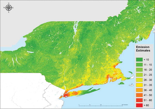
Figure 4 depicts emissions predicted over the period of 2002 to 2013 in the U.S. Northeast. We observed emission hotspots with more than 35 tons/year/km² in most highly populated areas such as Boston, MA, New York City, NY, and Long Island. In addition, we observed transportation emissions along major highways. Finally, we predicted low emission levels for rural areas (<20 tons/year/km²).

Figure 4. Estimated emission in U.S. Northeast.

Figure 5 shows the estimated emissions, land cover, and population distributions in the Greater Boston, MA, New York, NY, and Providence, RI, areas. In general, we found similar spatial patterns among highly populated areas such as Greater Boston and New York, reflecting typical urban activities. PEIRS predicted high emissions levels in developed areas (Figures 5d and 5e, colored red) in eastern Boston, New York City, and Long Island areas, with a mixture sources including residential heating, transportation, industrial, and commercial activities. More importantly, we were able to capture intra-urban variation. For example, we predicted lower emissions for eastern Cambridge, MA, where the Massachusetts Institute of Technology (MIT) campus is located. As shown in Figure 5a, emissions are noticeably lower (25–30 tons/year/km²) as opposed to surrounding areas such as Somerville and western Cambridge. The campus area is less populated compared to neighboring cities and the school has been actively promoting green building and energy sustainability programs over the past decade, which both contribute to lower emissions. Furthermore, we predicted high emissions at densely populated and commercially active areas in northern Brookline, MA, and lower emissions at parks, large green spaces, and residential areas in the southwestern part of the town (Figure 5a). Our results in New York (Figure 5b) show an intra-urban spatial pattern of PM_2.5 comparable to those reported by a previous study (Clougherty et al., 2013). Clougherty et al. found that large combustion boilers for residential heating, mostly burning oil, are concentrated in midtown and downtown Manhattan, NY, as well as in some neighborhoods of Brooklyn and Queens, NY. These areas are all highly developed with similar population density and land use. Even surrounded by high-intensity emission sources, we are able to identify intense oil-burning emissions in some of the grid cells that exceeded 60 tons/year/km² in these neighborhoods.

Figure 5. Estimated emission in (a) Greater Boston, MA, (b) New York, NY, and (c) Providence, RI. Land cover type from NLCD 2011 database in (d) Greater Boston, (e) New York, and (f) Providence. Population of year 2000 in (g) Greater Boston, (h) New York, and (i) Providence.

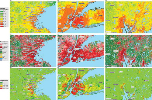
Our model overestimated emissions in areas surrounded by water surfaces or wetlands, such as Providence, RI, and southeastern Massachusetts (Figure 5c). For instance, the model estimated high emissions (20–30 tons/year/km²) in some green areas of southeastern Massachusetts where anthropogenic sources are scarce. The possible overestimation is likely due to bias in AOD readings, as the MAIAC algorithm was developed to retrieve AOD over land and is less reliable for retrievals over water surfaces (Lyapustin et al., 2011). Although we excluded pixels encompassing bodies of water prior, AOD retrieval near water or the shore can still be influenced by high humidity or ocean glint. Because we estimated PM_2.5 concentrations using AOD data, biases in the AOD are likely to influence the final emission product as well. However, it is also possible that some of the predicted emissions are due to primary or secondary particles from natural sources.

Land use regression

Predicted emissions in the northeast United States are related to land use variables (R² = 0.65). Table 2 shows the predicted land-use-specific emissions where the predominant sources include developed area (high/medium/low density and open area), traffic, and population. The land use regression model predicts that large point sources emit on average 0.58 tons/year/km², which is close to the averaged NEI point emission in 2008 (0.53 tons/year) and 2011(0.26 tons/year). Figure 6a shows the residuals (25th percentile = –2.7, mean = 0, 75th percentile = 2.5) of the land use regression model in the study area. As noted, the Providence, RI, and southeastern Massachusetts areas have larger residuals (>5 tons/year/km²), which suggests that either the predicted emissions are overestimated or they are not correlated to land use covariates, for example, biogenic sources, biogenic precursorsm or oceanic particles. Previous studies suggest that in remote areas most particles are secondary ones (Kanakidou et al., 2000; Spracklen et al., 2006; Andreae, 2007), which are not accounted for by land use models.

Table 2. LUR estimated emission from different land use for U.S. Northeast.

Land use type/emission sources		Averaged emission (ton/yr/km^2)
On road	A1–A3 major road	0.4 ~ 28
Developed area	High density	13
	Medium density	13
	Low density	6.7
	Open area	5.6
Population	250 people/cell	0.1
	10,000 people/cell	2.7
Farms	Crop and livestock	0.34
NEI point source	(NEI 2008 mean = 0.53)	0.58
Model R^2 = 0.65

Figure 6. Residual map of land use regression (LUR) model in (a) the U.S. Northeast and (b) Massachusetts. The residuals are emissions that are not related to land use parameters.

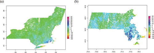
In addition to the national land cover product, we also incorporated the land cover data classified by the Massachusetts Department of Environmental Protection (Mass DEP), and fitted a separate land use model for Massachusetts. Compared to the national model(R² = 0.65), the Massachusetts model has a slightly higher R² of 0.67. As shown in Table 3, transportation, developed area, and population are the larger sources predicted by the land use model. With a finer classification, we can see the intra-urban variation related to industrial, residential, and commercial sources areas, which is not for the NEI database, mostly county-level averages (Figure 7b and 7c). Crop and livestock farms emissions are 0.7 tons/year/km², values similar to those reported by the NEI program. Cranberry bogs, nurseries, and orchards generate more emissions than other croplands. Consistent with the results of the U.S. Northeast land use regression, we observed high residuals in southeastern Massachusetts. As noted earlier, this may be due to difficulties in measuring AOD near water bodies, or possibly to the presence of sources whose emissions are independent of land use variables.

Table 3. LUR estimated emission from different land use for Massachusetts.

Land use type/emission sources		Averaged emission (ton/yr/km^2)
On road	A1–A3 major road	0.4–24.5
	Public transit	2.5
Developed area	High-density residential	3.6
	Medium-density residential	3.5
	Low-density residential	1.8
	Multifamily residential	2.1
	Open area	2.4
	Industrial	4.3
	Mining	2.4
	Commercial	3.1
	Junkyard	4.6
Population	400 people/cell	0.32
	10,000 people/cell	8
Farms	Crop and livestock	0.7
	Cranberry bog, nursery, orchard gardens	2.2–7.8
NEI point source		1.5
Model R^2 = 0.67

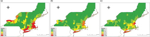
Figure 7. (a) Estimated emission vs. EPA NEI nonpoint emission in (b) 2008 and (c) 2011 at county level.

County-level evaluation

We found a moderate correlation between predicted and 2008 NEI emissions (R² = 0.52, CV = 144%). The slope and intercept of the 2008 NEI county model (β₁ = 2.6, β₀ = –38.7) suggest that the model underestimated the county-level emissions. Since the NEI emission data are right skewed (median = 4.9, mean = 11.8), we suspect the large error is due to extreme values (or outliers) in the NEI data. When restricting NEI data to less than 50 tons/year/km², we obtained a better model fit (R² = 0.66, CV = 20.0%, β₁ = 0.65, and β₀ = –5.6). This suggests that the model may underestimate the largest emission sources. The different temporal scale among emission predictions and NEI estimates could be another source of uncertainty leading to larger error and a larger deviation of the intercept. Nonetheless, the PEIRS method has great potential in predicting emissions at finer temporal scales and would reduce the temporal inconsistency error. We found similar results when comparing model emission predictions to those reported by the 2011 NEI. The model fit was significantly improved after removing high NEI emissions from the model (R² = 0.65 → 0.71, CV= 105% → 17.9%, β₁ = 3.4 → 1.09, β₀ = –47.8 → –11.7, all data → subset). Interestingly, the slope of the county regression model shows that our model overestimated emissions in comparison to the 2008 NEI, and slightly underestimated them when in comparison to the 2011 NEI. This is consistent with the emission changes documented in the 2011 NEI report, where emissions overall increased by 25 to 250% compared to 2008 due to resuspension of road dust and more frequent wildfires (EPA, 2011).

Table 4 and Table 5 show the state-specific county-level evaluation results compared to 2008 and 2011 NEI data, respectively. We observed fair agreement for Connecticut and New Hampshire compared to that for states with large sources such as New York and Massachusetts. In general, the agreement was improved when outliers were removed from the analysis. Predicted emissions were weakly related to NEI data in Vermont, suggesting that the model is less sensitive to low-level emission variations. As shown in Figure 7, for most counties in Vermont both model-predicted and NEI-reported emissions are low. The relatively high emissions predicted for Grand Isle County, Vermont, which is surrounded by Lake Champlain, may be due to water bias in the AOD. In addition, we did not find a good agreement for Franklin, Chittenden, and Addison counties of Vermont where the model predicts higher emissions (6–15 tons/year/km²) than those reported by NEI (< 5 tons/year/km²). However, we found that emissions of particles precursors such as NH₃, NO_x, and VOC are relatively high in these three counties according to the NEI 2008 report. Therefore, it is possible that differences are due to the formation of secondary particles and high-biomass burning sources, which are accounted for by the model but not included in the NEI database. In fact, counties where predicted emissions are higher than those reported by the NEI are locations with high precursor emissions. These include urban counties in Greater Boston, MA, New Haven, CT, New York City, NY, and Long Island, NY, as well as agriculture-driven counties in upper western New York state.

Table 4. Evaluation results of estimated emission vs. EPA NEI emission 2008 at county level.

	R^2	CV	Slope (β1)	Intercept (β0)
Connecticut	0.85	6.61%	0.73	–6.8
Maine	0.65	9.11%	0.54	–5.5
New Hampshire	0.86	15.0%	1.44	–15.5
Massachusetts	0.58 (0.87)	75.4% (6.97%)	1.84 (0.47)	–26.8 (1.0)
Rhode Island	0.21	13.3%	0.20	5.03
New York	0.58 (0.67)	211.1% (26.3%)	2.99 (0.71)	–45.44 (–6.6)
Vermont	0.01	7.45%	0.02	3.40

Note. Values in parentheses are model parameters when data are restricted to counties with ≤50 tons/yr NEI emission.

Table 5. Evaluation results of emission estimates vs. EPA NEI emission 2011 at county level.

	R^2	CV	Slope (β1)	Intercept (β0)
Connecticut	0.88	7.15%	1.41	–11.7
Maine	0.70	7.69%	0.76	–8.87
New Hampshire	0.89	8.13%	1.35	–14.6
Massachusetts	0.63 (0.27)	60.1% (16.1%)	2.37 (0.43)	–32.3 (3.7)
Rhode Island	0.49	10.7%	0.50	–0.47
New York	0.70 (0.80)	159.6% (21.2%)	3.80 (1.26)	–54.7 (–14.3)
Vermont	0.08	6.98%	0.11	1.96

Note. Values in parentheses are model parameter when data is restricted to counties with ≤50 tons/yr NEI emission.

Conclusions

In this paper, we have proposed a new method (the PEIRS approach) to construct spatially resolved emission inventories for fine particulate matter. The predicted emissions in the U.S. Northeast are in reasonable agreement with those reported in the 2008 and 2011 NEI. Our model can capture small-scale intra-urban variations in emissions and formation of secondary particles. Although inherent biases from the satellite data, possibly due to humidity interference and ocean glint, may reduce model accuracy, generally they manifest in remote areas with little population. Future research should examine whether the allegedly higher emissions are due to AOD measurement artifacts or the presence of secondary particles formed from biogenic precursors.

Overall, we have demonstrated the potential of satellite AOD data to predict PM_2.5 emissions at a fine spatial scale (1 km × 1 km). In contrast to conventional methods collecting emission data for known sources, we developed a model, based on the physical properties of particles, that captures emissions from all sources within a specific area. We can take advantage of the breadth of satellite-based remote sensing data to predict emission with high spatial and temporal resolution at low cost. As satellite remote sensing improves, more robust data with better temporal and spatial resolution will become available for predicting emissions not just for particles but for different gaseous air pollutants.

Acknowledgment

We especially thank Joy Lawrence and Alice Smythe for their comments and review of drafts.

Funding

This publication was made possible by U.S. EPA grant RD83479801. Its contents are solely the responsibility of the grantee and do not necessarily represent the official views of the U.S. EPA. Further, the U.S. EPA does not endorse the purchase of any commercial products or services mentioned in the publication.

Additional information

Funding

This publication was made possible by U.S. EPA grant RD83479801. Its contents are solely the responsibility of the grantee and do not necessarily represent the official views of the U.S. EPA. Further, the U.S. EPA does not endorse the purchase of any commercial products or services mentioned in the publication.

Notes on contributors

Chia-Hsi Tang

Chia-Hsi Tang is a Doctor of Science student in the Department of Environmental Health, Harvard School of Public Health.

Brent A. Coull

Brent A. Coull is a professor of the Department of Biostatistics, Harvard School of Public Health.

Joel Schwartz

Joel Schwartz is a professor of the Department of Environmental Health, Harvard School of Public Health.

Alexei I. Lyapustin

Alexei I. Lyapustin is a physical research scientist at the Climate and Radiation Laboratory at NASA.

Qian Di

Qian Di is a Doctor of Science student in the Department of Environmental Health, Harvard School of Public Health.

Petros Koutrakis

Petros Koutrakis is a professor of the Department of Environmental Health, Harvard School of Public Health.

References

- Andreae, M.O. 2007. Atmosphere. Aerosols before pollution. Science 315(5808):50–51. doi:10.1126/science.1136529.
- Chudnovsky, A., C. Tang, A. Lyapustin, Y. Wang, J. Schwartz, and P. Koutrakis. 2013. A critical assessment of high-resolution aerosol optical depth retrievals for fine particulate matter predictions. Atmos. Chem. Phys. 13(21):10907–17. doi:10.5194/acp-13-10907-2013.
- Clougherty, J.E., I. Kheirbek, H.M. Eisl, Z. Ross, G. Pezeshki, J.E. Gorczynski, S. Johnson, S. Markowitz, D. Kass, and T. Matte. 2013. Intra-urban spatial variability in wintertime street-level concentrations of multiple combustion-related air pollutants: the New York City Community Air Survey (NYCCAS). J. Expos. Sci. Environ. Epidemiol. 23(3):232–40. doi:10.1038/jes.2012.125.
- Donateo, A., and D. Contini. 2014. Correlation of dry deposition velocity and friction velocity over different surfaces for PM2.5 and particle number concentrations. Adv. Meteorol. 2014:1–12. doi:10.1155/2014/760393.
- Duncan, B.N., A.I. Prados, L.N. Lamsal, Y. Liu, D.G. Streets, P. Gupta, E. Hilsenrath, R.A. Kahn, J.E. Nielsen, A.J. Beyersdorf, S.P. Burton, A.M. Fiore, J. Fishman, D.K. Henze, C.A. Hostetler, N.A. Krotkov, P. Lee, M. Lin, S. Pawson, G. Pfister, K.E. Pickering, R.B. Pierce, Y. Yoshida, and L.D. Ziemba. 2014. Satellite data of atmospheric pollution for U.S. air quality applications: Examples of applications, summary of data end-user resources, answers to FAQs, and common mistakes to avoid. Atmos. Environ. 94:647–62. doi:10.1016/j.atmosenv.2014.05.061.
- Gupta, P., and S.A. Christopher. 2009. Particulate matter air quality assessment using integrated surface, satellite, and meteorological products: 2. A neural network approach. J. Geophys. Res. 114(D20). doi:10.1029/2008jd011497.
- Hoff, R., and S. Christopher. 2009. Remote sensing of particulate pollution from space: Have we reached the promised land? J. Air Waste Manage. Assoc. 59(6):645–75. doi:10.3155/1047-3289.59.6.645.
- Hu, X., L.A. Waller, A. Lyapustin, Y. Wang, M.Z. Al-Hamdan, W.L. Crosson, M.G. Estes, S.M. Estes, D.A. Quattrochi, S.J. Puttaswamy, and Y. Liu. 2014. Estimating ground-level PM2.5 concentrations in the southeastern United States using MAIAC AOD retrievals and a two-stage model. Remote Sens. Environ. 140:220–32. doi:10.1016/j.rse.2013.08.032.
- Kalnay, E., M. Kanamitsu, R. Kistler, W. Collins, D. Deaven, L. Gandin, M. Iredell, S. Saha, G. White, J. Woollen, Y. Zhu, A. Leetmaa, R. Reynolds, M. Chelliah, W. Ebisuzaki, W. Higgins, J. Janowiak, K. C. Mo, C. Ropelewski, J. Wang, R. Jenne, and D. Joseph. 1996. The NCEP/NCAR 40-year reanalysis project. Bull. Am. Meteorol. Soc. 77:437–71. doi:10.1175/1520-0477(1996)077<0437:TNYRP>2.0.CO;2.
- Kanakidou, M., K. Tsigaridis, F.J. Dentener, and P.J. Crutzen. 2000. Human-activity-enhanced formation of organic aerosols by biogenic hydrocarbon oxidation. J. Geophys. Res. 105(D7): 9243. doi:10.1029/1999jd901148.
- Kloog, I., A.A. Chudnovsky, A.C. Just, F. Nordio, P. Koutrakis, B.A. Coull, A. Lyapustin, Y. Wang, and J. Schwartz. 2014. A new hybrid spatio-temporal model for estimating daily multi-year PM2.5 concentrations across northeastern USA using high resolution aerosol optical depth data. Atmos. Environ. 95:581–90. doi:10.1016/j.atmosenv.2014.07.014.
- Kloog, I., P. Koutrakis, B. A. Coull, H.J. Lee, and J. Schwartz. 2011. Assessing temporally and spatially resolved PM2.5 exposures for epidemiological studies using satellite aerosol optical depth measurements. Atmos. Environ. 45(35):6267–75. doi:10.1016/j.atmosenv.2011.08.066.
- Lee, H. J., B.A. Coull, M.L. Bell, and P. Koutrakis. 2012. Use of satellite-based aerosol optical depth and spatial clustering to predict ambient PM2.5 concentrations. Environ. Res. 118:8–15. doi:10.1016/j.envres.2012.06.011.
- Lepeule, J., F. Laden, D.W. Dockery, and J.D. Schwartz. 2012. Chronic exposure to fine particles and mortality: An extended follow-up of the Harvard Six Cities study from 1974 to 2009. Environ. Health Perspect. 120:965–970.
- Liu, Y., C.J. Paciorek, and P. Koutrakis. 2009. Estimating regional spatial and temporal variability of PM(2.5) concentrations using satellite data, meteorology, and land use information. Environ. Health Perspect. 117(6):886–92. doi:10.1289/ehp.0800123.
- Lyapustin, A., Y. Wang, I. Laszlo, R. Kahn, S. Korkin, L. Remer, R. Levy, and J.S. Reid. 2011. Multiangle implementation of atmospheric correction (MAIAC): 2. Aerosol algorithm. J. Geophys. Res. 116:D03211. doi:10.1029/2010jd014986.
- Martin, R.V. 2008. Satellite remote sensing of surface air quality. Atmos. Environ. 42(34):7823–43. doi:10.1016/j.atmosenv.2008.07.018.
- Mesinger, F., G. DiMego, E. Kalnay, K. Mitchell, P.C. Shafran, W. Ebisuzaki, D. Jović, J. Woollen, E. Rogers, E.H. Berbery, M.B. Ek, Y. Fan, R. Grumbine, W. Higgins, H. Li, Y. Lin, G. Manikin, D. Parrish, and W. Shi. 2006. North American regional reanalysis. Bull. Am. Meteorol. Soc. 87(3):343–60. doi:10.1175/bams-87-3-343.
- Pope, C.A. 3rd, R.T. Burnett, M.J. Thun, E.E. Calle, D. Krewski, K. Ito, and G.D. Thurston. 2002. Lung cancer, cardiopulmonary mortality, and long-term exposure to fine particulate air pollution. J. Am. Med. Assoc. 287(9):1132–41. doi:10.1001/jama.287.9.1132
- Ren, C., G.M. Williams, and S. Tong. 2006. Does particulate matter modify the association between temperature and cardiorespiratory diseases? Environ. Health Perspect. 114:1690–1696. doi:10.1289/ehp.9266.
- Schwartz, J. 2001. Is there harvesting in the association of airborne particles with daily deaths and hospital admissions? Epidemiology (Cambridge, Mass.) 12:55–61. doi:10.1097/00001648-200101000-00010
- Schwartz, J., and D.W. Dockery. 1992. Increased mortality in Philadelphia associated with daily air pollution concentrations. Am. Rev. Respir. Dis. 145(3):600–4. doi:10.1164/ajrccm/145.3.600
- Schwartz, J., F. Laden, and A. Zanobetti. 2002. The concentration-response relation between PM(2.5) and daily deaths. Environ. Health Perspect. 110:1025–29. doi:10.1289/ehp.021101025
- Spengler, J.D., J.M. Samet, and J.F. McCarthy. 2001. Indoor air quality handbook. New York, NY: McGraw-Hill.
- Spracklen, D.V., K.S. Carslaw, M. Kulmala, V.M. Kerminen, G.W. Mann, and S.L. Sihto. 2006. The contribution of boundary layer nucleation events to total particle concentrations on regional and global scales. Atmos. Chem. Phys. 6(12):5631–48. doi:10.5194/acp-6-5631-2006.
- Turner, M.C., D. Krewski, C.A. Pope 3rd, Y. Chen, S.M. Gapstur, and M.J. Thun. 2011. Long-term ambient fine particulate matter air pollution and lung cancer in a large cohort of never-smokers. Am. J. Respir. Crit. Care Med. 184:1374–81. doi:10.1164/rccm.201106-1011OC.
- United States Environmental Protection Agency [EPA]. 2001. Sources and sinks of PM10 in the San Joaquin Valley. https://www.arb.ca.gov/research/apr/reports/l2022.pdf
- United States Environmental Protection Agency [EPA]. 2008. 2008 National Emissions Inventory: Review, analysis and highlights. ftp://ftp.epa.gov/EmisInventory/2008v3/doc/evaluate2008nei_rtr_finalreport20121220.pdf
- United States Environmental Protection Agency [EPA]. 2011. Profile of the 2011 National Air Emissions Inventory. https://www.epa.gov/sites/production/files/2015-08/documents/lite_finalversion_ver10.pdf
- Vehkamaki, H., and I. Riipinen. 2012. Thermodynamics and kinetics of atmospheric aerosol particle formation and growth. Chem. Soc. Rev. 41(15):5160–73. doi:10.1039/c2cs00002d.
- Zanobetti, A., and J. Schwartz. 2006. Air pollution and emergency admissions in Boston, MA. J. Epidemiol. Commun. Health 60:890–95. doi:10.1136/jech.2005.039834.