
ABSTRACT
Exposure to traffic emission is harmful to human health. Emission inventories are essential to public health policies aiming at protecting human health, especially in areas with incomplete or nonexistent air pollution monitoring networks. In Brazil, for example, only 1.7% of municipal districts have a monitoring network, and only a few studies have reported data on vehicle emission inventories. No studies have presented emission inventories by municipality. In this study, we predicted vehicular emissions for 5570 municipal districts in Brazil during the period 2001–2012. We used a top-down method to estimate emissions. Carbon dioxide (CO2) is the pollutant with the highest emissions, with approximately 190 million tons per year during the period 2001–2012). For the other traffic-related pollutants, we predicted annual emissions of 1.5 million tons for carbon monoxide (CO), 1.2 million tons of nitrogen oxides (NOx), 209,000 tons of nonmethane hydrocarbons (NMHC), 58,000 tons of particulate matter (PM), and 42,000 tons for methane (CH4). From 2001 to 2012, CO, NMHC, and PM emissions decreased by 41, 33, and 47%, respectively, whereas those CH4, NOx, and CO2 increased by 2, 4, and 84%, respectively. We estimated uncertainties in our study and found that NOx was the pollutant with the lowest percentage difference, 8%, and NMHC with the highest one, 30%. For CO, CH4, CO2, and PM, the values were 22, 14, 21, and 20%, respectively. Finally, we found that during 2001 and 2012 emissions increased in the Northwest and Northeast. In contrast, pollutant emissions, except for CO2, decreased in the Southeast, South, and part of Midwest. Our predictions can be critical to efforts developing cost-effective public policies tailored to individual municipal districts in Brazil.
Implications: Emission inventories may be an alternative approach to provide data for air quality forecasting in areas where air quality data are not available. This approach can be an effective tool in developing spatially resolved emission inventories.
Introduction
Motor vehicle emissions are a key contributor to air pollution (Lelieveld et al., Citation2015). Globally, in urban areas, vehicular emissions account for 25% of the ambient PM2.5 (particulate matter with an aerodynamic diameter <2.5 μm) concentrations (Karagulian et al., Citation2015). In addition, Sokhi (Citation2011) suggested that motor vehicle emissions are responsible for 30% of nitrogen oxides (NOx), 14% of carbon dioxide (CO2), 54% of carbon dioxide (CO), and 47% of nonmethane hydrocarbons (NMHC) of global emissions.
Epidemiological studies have demonstrated that these traffic-related air pollutants are a risk factor for increased morbidity and early mortality (Svendsen et al., Citation2012; Gonzalez-Barcala et al., Citation2013; Williams et al., Citation2009; Keuken et al., Citation2012; Buonanno et al., Citation2013; Chen et al., Citation2012; Lelieveld et al., Citation2015). In Brazil, exposure to air pollutants has been associated with increased lung cancer occurrences (Fajersztajn et al., Citation2013), cardiorespiratory diseases (Paula Santos et al., Citation2005), asthma (Amâncio and Nascimento, Citation2012), and premature deaths (Lin et al., Citation2004).
Air pollution concentration data are essential for controlling source emissions and protecting human health. Ideally, these data are obtained from air pollution monitoring networks (Adams and Kanaroglou, Citation2016; Kanaroglou et al., Citation2005; Zheng et al., Citation2011). However, most developing countries do not have monitoring networks or have inadequate networks. For example, in Brazil, there are a total of 5570 municipal districts, but only 1.7% of them have an air pollution monitoring network (Alves et al., Citation2014). Brazil has 1.3 stations per million inhabitants, whereas the USA has 16 stations (Alves et al., Citation2014), Japan has 15 stations (Fukushima, Citation2006), and Germany has 23 stations (German Environment Agency [UBA], Citation2013).
Emission inventories may be an alternative approach to provide data for air quality forecasting in areas where air quality data are not available (Smit et al., Citation2008; Lozhkina and Lozhkin, Citation2015; Coelho et al., Citation2014; Bandeira et al., Citation2011). In Brazil, only a few studies have reported information on vehicle emission inventories (Réquia et al., Citation2015; Ueda and Tomaz, Citation2011; Gallardo et al., Citation2012; Duarte et al., Citation2013). However, these investigations have only presented results for specifics cities, such Brasília (Brazil’s capital), São Paulo (the biggest Brazilian city), and Rio de Janeiro. To our knowledge, the exception is a study for South America (Alonso et al., Citation2010), which the authors estimated emissions based on the analysis and aggregation of available inventories for major cities. Due to limited number of local inventories, Alonso et al. (Citation2010) extrapolated vehicle emissions based on the vehicle density, urban population, and socioeconomic factors. In Brazil, most of the emission inventories are estimated by the Brazilian Environmental Agency (national inventories) and the state environmental agencies (state or regional inventories). To date, only a few state environmental agencies in Brazil have reported emission data. Most of the regions in the North, Northeast, and Midwest do not have emission inventories.
In this study, we predict vehicular emissions for 5570 municipal districts in Brazil, spanning throughout the country during the period between 2001 and 2012.
Materials and methods
Study area
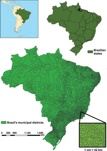
Brazil has approximately 200 million inhabitants and covers a surface of 8,515,767 km2 divided into 26 states and a federal district. The states are further subdivided into 5570 municipal districts (). The largest three cities, São Paulo, Rio de Janeiro and Salvador, have populations of 10,009,000, 5,613,000, and 2,331,000, respectively. Regional transit and public transit across Brazil vary in their quality of services between states. The national highways/freeway system includes 2 million kilometers of roads, of which approximately 200,000 km are paved.
Figure 1. Study area.
Vehicle emission inventory
We chose a top-down approach for predicting emissions, and we used the following equation:
where E are the annual emissions in metric tons; Vf is the number of vehicles; α is fraction of fleet in use; Dt is the average distance traveled in km/yr; Ef is the emission factor in grams of pollutant per unit distance (g/km); x is the municipal district (5570); i is the year considered to estimate emissions (from 2001 to 2012); z is the pollutant type; and y is the vehicle type.
We predicted emissions for carbon monoxide (CO), nonmethane hydrocarbons (NMHC), methane (CH4), nitrogen oxides (NOx), particulate matter (PM), and carbon dioxide (CO2). For PM emissions, we considered the sum of emissions (exhaust, brakes, tires, and pavement wear). For CH4 and NMHC, we accounted for only evaporative emissions. Furthermore, we considered six vehicle categories: light vehicles (passenger cars), utility vehicles (for transport of passengers or goods), motorcycles, trucks (light, middle, and heavy duty), urban buses, and interstate buses. In Appendix 1 (Supplemental Material), we present the characteristics each vehicle type. Finally, to estimate the total emissions of a pollutant z for year i, and for municipal district x, we used the following equation:
where TAE are the emissions, in tons, for light vehicles (Lv), utility vehicles (Uv), motorcycles (Mo), trucks (Tr), urban buses (Ub), and interstate buses (Ib).
Vehicle fleet (Vf)
Vehicle fleet data were obtained from Brazil’s National System of Traffic (NST) (Denatran, Citation2015). NST considers buses as unique category. According to the Brazilian Environmental Agency (MMA, Citation2013), 10% of the buses are interstate and 90% are urban.
The vehicle fleet data include all vehicles owned in a municipal district rather than the fleet in use. For our analysis, we excluded vehicles that were no longer in use (old vehicles) and vehicles purchased in the municipal district but used in another. To determine the vehicles in use, we multiplied the NST emission data by the fraction of vehicles in use, α, as recommended by the Brazilian Environmental Agency, which considers the vehicle age and type. The value α is based on a scrapping curve. For example, the Brazilian Environmental Agency recommends an α value equal to 0.95 for light vehicles with ≤5 yr. It means that 95% of the light vehicles with ≤5 yr are in use. Since it was not possible to determine the fleet age, we assumed a median age for vehicles <20 yr (according to NST, 95% of vehicles have a maximum age of 20 yr). Specifically, we used the following multipliers for active vehicles for α: light vehicles (0.85), utility vehicles (0.75), motorcycles (0.55), trucks (0.80), urban buses (0.85), and interstate buses (0.85).
Distance traveled (Dt)
We obtained distance traveled data from the Brazilian Environmental Agency (MMA, Citation2013). According to the agency, the distance traveled depends on the both vehicle age and type. As mentioned previously, it was not possible to obtain data on vehicle age. Therefore, we calculated an average use for vehicles between 0 and 20 yr old, which are 13,524 km/yr for light vehicles, 14,524 km/yr for utility vehicles, 7714 km/yr for motorcycles; 67,366 km/yr for trucks, 69,857 km/yr for urban buses, and 194,048 km/yr for interstate buses. In the supplemental Appendix 1, we present the data set provided by the Brazilian Environmental Agency.
Emission factor (Ef)
We obtained emission factor data from the Brazilian Environmental Agency (MMA, Citation2013) and Environmental Agency of São Paulo (CETESB, Citation2012). The emission factor is a function of vehicle age, and we adopted the same procedure as for distance traveled. Appendices 2 and 3 present emission factors for vehicle type (y), pollutant (z), and year (i) used in our study.
Evaluation of the emission inventories
We compared our predictions with those reported in the National Emission Inventory by the Brazilian Environmental Agency (MMA, Citation2013). We performed two comparisons using results from E (eq 1) and TAE (eq 2), respectively.
Since the national inventory reports total emissions for the entire country, there is no spatial disaggregation by state or municipal district. Consequently, we used the sum of emission from all 5570 municipal districts to evaluate emission predictions using the following equations:
where TEB’ is the total emission in Brazil considering all type of vehicles; TEB’’ is the total emission in Brazil per type of vehicle; and N is the number of municipal districts. Finally, we evaluated our results as the following equations:
where ER′ is the evaluation of emission considering all vehicle types and BEA′ is the emissions for all vehicles types, which we obtained from the Brazilian Environmental Agency. Furthermore, ER″ is the evaluation of emissions considering the vehicles categories; and BEA″is the emissions per vehicles category, which we obtained from the Brazilian Environmental Agency as well.
The Brazilian Environmental Agency estimated the emissions using the same approach that we used, the top-down method. However, the agency estimates the emissions at the country level; there is no disaggregation by municipal districts.
Results and discussion
Descriptive analysis
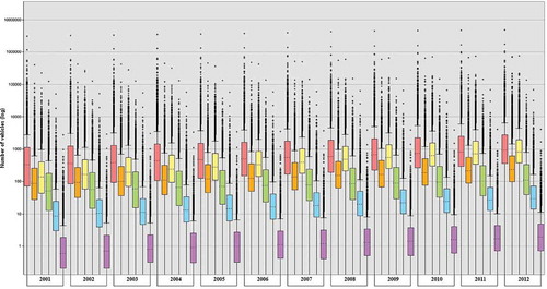
Light vehicles represent approximately 59% of the fleet. The respective numbers for motorcycles, utility vehicles, trucks, and buses (urban and interstate) are 28, 10, 2, and 1%. In 2001, the entire fleet in Brazil (all vehicles) comprised approximately 23 million vehicles. In 2012, the fleet doubled to approximately 46 million vehicles. Light vehicles increased by 72%, utility vehicles by 75%, motorcycles by 287%, trucks by 53%, urban buses by 52%, and interstate buses by 49%. shows a box-plot graph of vehicle numbers between 2001 and 2012. As noted above, we only considered vehicles in use to predict emissions, the number of which was lower than that of vehicles registered (76 million in 2012).
Figure 2. Number of vehicles during the period 2001–2012. Light vehicles (red); utility vehicles (orange); motorcycles (yellow); trucks (green); urban buses (blue); and interstate buses (purple).
The Brazilian fleet represents a non-negligible fraction of the global one. According to the World Health Organization (WHO), during the period 2000–2010, Brazil had the second largest fleet increase behind China (WHO, Citation2012). The Brazilian Energy Agency (EPE) reported that by 2050, the country fleet will increase by more than 300%, totaling an estimated 130 million registered vehicles (EPE, Citation2014). This will have an adverse impact on environmental quality, human health, and urban mobility (Ribeiro et al., Citation2014; Weber et al., Citation2014; Lima et al., Citation2014; Chandran et al., Citation2013).
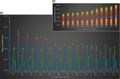
Light vehicles and trucks emit the highest amount of pollutants (). In 2012, for example, light vehicles were responsible for 48% of CO, 40% of NMHC, and 51% of CH4, whereas trucks were responsible for 58% of NOx and 47% of PM. Finally, light vehicles and trucks were responsible for 36% and 34% of CO2 emissions, respectively.
Figure 3. Air pollution inventories between 2001 and 2012 by vehicle and pollutant type. Emission inventories for (a) CO, NMHC, CH4, NOx, and PM and (b) CO2. Light vehicles (Lv); utility vehicles (Uv); motorcycles (Mo); trucks (Tr); urban buses (Ub); and interstate buses (Ib). There is a large difference for the scale of values between the CO2 and other pollutants. Therefore, we present the results for CO2 in a separate chart (b).
According to Gallardo et al. (Citation2012), vehicle age is an important parameter for determining emission by vehicles type, especially for the diesel fleet. Older vehicles emit more pollutants per distance. For example, the authors suggest that trucks are an important source of PM due to their age. On average, trucks are the oldest category of vehicles (Denatran, Citation2015). As mentioned above, in our study trucks were responsible for the highest emissions of PM.
As expected, CO2 was the pollutant with the highest emissions, approximately 190 million tons per year. For the other pollutants, we estimated an annual average of approximately 1.5 million tons of CO, 1.2 million tons of NOx, 209,000 tons of NMHC, 58,000 tons of PM, and CH4 presented the lowest emission, 42,000 tons.
Our findings are in agreement with other studies (Brondfield et al., Citation2012; Nejadkoorki et al., Citation2008; Nagpure and Gurjar, Citation2012). From 2001 to 2012, traffic emissions CO, NMHC, and PM decreased by 41, 33, and 47%, respectively, whereas those of CH4, NOx, and CO2 increased by 2, 4, and 84%, respectively. shows the temporal variation of emissions by vehicle and pollutant type.
The decline of CO, NMHC, and PM emissions is a result of the implemented emission control strategies over the last 30 yr, for example, the national program of air quality control (PRONAR) and the program to control vehicular emissions (PROCONVE). The benefits of these environmental policies have been reported by other emission inventory studies, such as Gallardo et al. (Citation2012) and Vlachokostas et al. (Citation2009). In contrast, the PRONAR and PROCONVE programs do not include regulations for CO2 emissions. This and the fleet growth are the main reasons for the dramatic increase in CO2 emissions between 2001 and 2012.
Evaluation of uncertainties in emissions
We estimated uncertainties in emissions and found that urban and interstate buses were the category with the highest values, 67% and 65%, respectively, and trucks with the lowest value, 16%. The respective estimates for light vehicles, utility vehicles, and motorcycles were 29, 49, and 46%. In Appendices 4–9 (Supplemental Material) we compare our predictions by vehicle and pollutant type with those reported in the National Emission Inventory by the Brazilian Environmental Agency.
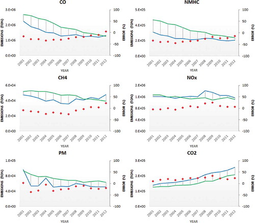
NOx was the pollutant with the lowest percent different, 8%, and NMHC with the highest one, 30%. For CO, CH4, CO2, and PM, the values were 22, 14, 21, and 20%, respectively. In , we compare our predictions with those reported in the national inventory. Other studies have shown similar differences with national inventories. For example, Zhou et al. (Citation2014) estimated emissions for four cities in China and found an average difference of 39.9, 33.9, 46.3, and 46.9% for SO2, NOx, NMHC, and CO, respectively.
Figure 4. Comparison between our predictions and those reported in the Brazilian Environmental Agency national inventory. This study (blue line); national inventory (green line); and difference (red dots). CO2 emissions are at 103 tons.
Spatiotemporal distribution
and show the spatiotemporal variability in emission inventories during the period 2001–2012. Emissions increased in the Northwest and Northeast. In contrast, pollutant emissions, except for CO2, decreased in the Southeast, South, and part of Midwest. CO2 emissions (, map B) increased significantly throughout the country. In Appendices 10–15, we present maps of spatiotemporal distribution with better scale for visualization.
Figure 5. Spatiotemporal distribution of emission inventories of CO, NMHC, CH4, and NOx (tons/year). Emissions of (a) CO; (b) NMHC; (c) CH4; and (d) NOx. The values are log-normalized.
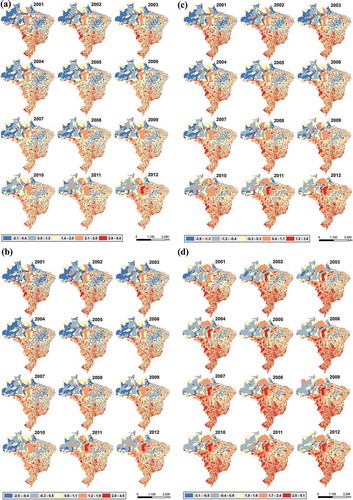
Figure 6. Spatiotemporal distribution of emission inventories of PM and CO2 (tons/year). Emissions of (a) PM and (b) CO2. The values are log-normalized.
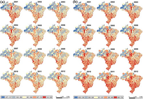
The fleet growth rate in Brazil between 2001 and 2012 differed by economic region. The northern part of the country is less affluent than the southern one. As result, parts of the Midwest, Southeast, and South have approximately 85% of the national fleet. However, recently, the fleet has increased in most of the municipal districts in the Northwest and Northeast due to strong economic growth. The fleet growth rates for the different regions, during the period 2001–2012, were as follows: 140% for the Northeast, 187% for the Northwest, 133% for the Midwest, 91% for the Southeast, and 105% for the South 105%.
Other studies have shown that association economic factors are important variables to distinguish spatial variability of fleet growth and traffic emissions. Austin et al. (Citation2013), for example, identified high association in particle composition in the United States based on geographic locations, emission profiles, population, and economic variables. Zou et al. (Citation2014) examined spatial cluster of air pollution exposure across the United States and suggest economic variables as significant components.
Limitations
Our study has a few limitations. We did not have data on fleet age; instead, we used the rate α and data on the average number of vehicles in use from the Brazilian Traffic Agency. In addition, we had no data on the diurnal variation of emissions and emissions from cold start or idling periods. Finally, we were unable to distinguish the type of fuel (gasoline or alcohol) for the light and utility vehicles.
Conclusions
There are no studies predicting emission inventories in Brazil at the municipality level. This is an important first step in understanding contributions and finding solutions to environmental problems, especially in areas without air pollution monitoring network. Brazil has a rapidly growing fleet, and its emissions contribute significantly to South America and even at a global level. Our approach can be an effective tool in developing spatially resolved emission inventories; this enables us to develop mitigation strategies tailored to specific municipal districts in Brazil. Our findings have identified spatial differences of municipal districts, which warrant the attention of policy makers and environmental agencies at local, regional, and national levels. Further investigations may assess spatial patterns of traffic emissions in order to understand the geographic phenomena. This analysis is important to identify groups of municipal districts with varying levels of traffic emissions.
Appendix_Vehicular_emisisions_in_Brazil_v.4.docx
Download MS Word (7 MB)Funding
This publication was made possible by the U.S. Environmental Protection Agency (EPA) grant RD-834798. Its contents are solely the responsibility of the grantee and do not necessarily represent the official views of the EPA. Further, the EPA does not endorse the purchase of any commercial products or services mentioned in the publication.
Additional information
Funding
Notes on contributors
Weeberb J. Réquia
Weeberb J. Réquia is a researcher (postdoctoral fellow) at the School of Geography and Earth Sciences, McMaster University, Hamilton, Ontario, Canada.
Petros Koutrakis
Petros Koutrakis is a professor of environmental science at Harvard University, Cambridge, MA, USA.
Henrique Llacer Roig
Henrique Llacer Roig is a professor at the Geosciences Institute at the University of Brasília, Brasília, Brazil.
Matthew D. Adams
Matthew D. Adams is a researcher (postdoctoral fellow) at the School of Geography and Earth Sciences, McMaster University, Hamilton, Ontario, Canada.
Related Research Data
References
- Adams, M.D., and P.S. Kanaroglou. 2016. Mapping real-time air pollution health risk for environmental management: Combining mobile and stationary air pollution monitoring with neural network models. J. Environ. Manage. 168:133–141. doi: 10.1016/j.jenvman.2015.12.012.
- Alonso, M.F., K.M. Longo, S.R. Freitas, R. Mello da Fonseca, V. Marçal, M. Pirre, and L. Gallardo Klenner. 2010. An urban emissions inventory for south america and its application in numerical modeling of atmospheric chemical composition at local and regional scales. Atmos. Environ. 44:5072–5083. doi: 10.1016/j.atmosenv.2010.09.013.
- Alves, E.M.P., R.R. Costa, A.A. Braga, M. Miranda, N.C. do Nascimento, and P.H. Nascimento Saldiva. 2014. Monitoramento Da Qualidade Do Ar No Brasil. São Paulo: Instituto Saúde e Sustentabilidade.
- Amâncio, C.T., and L.F. Costa Nascimento. 2012. Asthma and ambient pollutants: A time series study. Rev. Assoc. Méd. Bras. 58:302–307. doi: 10.1016/S0104-4230(12)70199-9.
- Austin, E., B.A. Coull, A. Zanobetti, and P. Koutrakis. 2013. A framework to spatially cluster air pollution monitoring sites in US based on the PM2.5 composition. Environ. Int. 59:244–254. doi: 10.1016/j.envint.2013.06.003
- Bandeira, J.M., M.C. Coelho, M.E. Sá, R. Tavares, and C. Borrego. 2011. Impact of land use on urban mobility patterns, emissions and air quality in a Portuguese medium-sized city. Sci. Total Environ. 409:1154–1163. doi: 10.1016/j.scitotenv.2010.12.008.
- Brazilian Energy Agency (EPE). 2014. Demanda de Energia, 1st ed. Brasilia: Ministério de Minas e Energia. http://www.epe.gov.br/Estudos/Documents/DEA 13-14 Demanda de Energia 2050.pdf (accessed December 10, 2015).
- Brazilian Environmental Agency (MMA). 2013. Inventário Nacional de Emissões Atmosféricas por Veículos Automotores Rodoviários: 2013 Ano-Base 2012, 1st ed. Brasília: Agência Nacional de Transporte Terrestre.
- Brondfield, M.N, L.R. Hutyra, C.K. Gately, S.M. Raciti, and S.A. Peterson. 2012. Modeling and validation of on-road CO2 emissions inventories at the urban regional scale. Environ. Pollut. 170:113–123. doi: 10.1016/j.envpol.2012.06.003
- Buonanno, G., G. Marks, and L. Morawska. 2013. Health effects of daily airborne particle dose in children: Direct association between personal dose and respiratory health effects. Environ. Pollut. 180:246–250. doi: 10.1016/j.envpol.2013.05.039.
- Chandran, A., G. Kahn, T. Sousa, F. Pechansky, D.M. Bishai, and A.A. Hyder. 2013. Impact of road traffic deaths on expected years of life lost and reduction in life expectancy in Brazil. Demography 50:229–236. doi: 10.1007/s13524-012-0135-7.
- Chen, R., H. Kan, B. Chen, W. Huang, Z. Bai, G. Song, and G. Pan. 2012. Association of particulate air pollution with daily mortality: The China Air Pollution and Health Effects Study. Am. J. Epidemiol. 11:1173–81. doi: 10.1093/aje/kwr425.
- Coelho, M.C., T. Fontes, J.M. Bandeira, S.R. Pereira, O. Tchepel, D. Dias, E. Sá, J.H. Amorim, and C. Borrego. 2014. Assessment of potential improvements on regional air quality modelling related with implementation of a detailed methodology for traffic emission estimation. Sci. Total Environ. 470–471:127–137. doi: 10.1016/j.scitotenv.2013.09.042.
- Denatran. 2015. Estatística de Veículos. www.denatran.gov.br (accessed December 10, 2015).
- Duarte, C., R. De Souza, S. Deodoro Silva, M. Aure, M. De Almeida D’Agosto, and A. Prado Barboza. 2013. Inventory of conventional air pollutants emissions from road transportation for the state of Rio de Janeiro. Energy Policy 25:125–135. doi: 10.1016/j.enpol.2012.10.021
- Environmental Agency of São Paulo (CETESB). 2012. Inventário de Emissões Das Fontes Estacionárias Do Estado de São Paulo. São Paulo: CETESB.
- Fajersztajn, L., M. Veras, L. Vizeu Barrozo, and P. Saldiva. 2013. Air pollution: A potentially modifiable risk factor for lung cancer. Nat. Rev. Cancer 13:674–678. doi: 10.1038/nrc3572.
- Fukushima, H. 2006. Air pollution monitoring in East Asia. Sci. Technol. Trends 14:958–67.
- Gallardo, L., J. Escribano, L. Dawidowski, N. Rojas, F.M. Andrade, and M. Osses. 2012. Evaluation of vehicle emission inventories for carbon monoxide and nitrogen oxides for Bogotá, Buenos Aires, Santiago, and São Paulo. Atmos. Environ. 47:12–19. doi: 10.1016/j.atmosenv.2011.11.051.
- German Environment Agency (UBA). 2013. Air Monitoring Networks. http://www.umweltbundesamt.de/en/topics/air/measuringobservingmonitoring/air-monitoring-networks (accessed November 1, 2016).
- Gonzalez-Barcala, F.J., S. Pertega, L. Garnelo, T.P. Castro, M. Sampedro, J.S. Lastres, M.A. San Jose Gonzalez, L. Bamonde, J.M. Carreira, and A.L. Silvarrey. 2013. Truck traffic related air pollution associated with asthma symptoms in young boys: A cross-sectional study. Public Health 127:275–281. doi: 10.1016/j.puhe.2012.12.028.
- Kanaroglou, P.S., M. Jerrett, J. Morrison, B. Beckerman, M.A. Arain, N.L. Gilbert, and J.R. Brook. 2005. Establishing an air pollution monitoring network for intra-urban population exposure assessment: A location-allocation approach. Atmos. Environ. 39:2399–2409. doi: 10.1016/j.atmosenv.2004.06.049.
- Karagulian, F., C.A. Belis, C. Francisco, C. Dora, A.M. Prüss-Ustün, S. Bonjour, H. Adair-Rohani, and M. Amann. 2015. Contributions to cities’ ambient particulate matter (PM): A systematic review of local source contributions at global level. Atmos. Environ. 120:475–483. doi: 10.1016/j.atmosenv.2015.08.087
- Keuken, M.P., S. Jonkers, P. Zandveld, M. Voogt, and S. van den Elshout. 2012. Elemental carbon as an indicator for evaluating the impact of traffic measures on air quality and health. Atmos. Environ. 61(December):1–8. doi: 10.1016/j.atmosenv.2012.07.009.
- Lelieveld, J., J. Evans, M. Fnais, D. Giannadaki, and A. Pozzer. 2015. The contribution of outdoor air pollution sources to premature mortality on a global scale. Nature 525:367–371. doi: 10.1038/nature15371
- Lima, J.P., R. da Silva Lima, and A.N. Rodrigues da Silva. 2014. Evaluation and selection of alternatives for the promotion of sustainable urban mobility. Procedia Soc. Behav. Sci. 162:408–418. doi: 10.1016/j.sbspro.2014.12.222.
- Lin, C.A., L.A.A. Pereira, D.C. Nishioka, G.M.S. Conceição, A.L.F. Braga, and P.H.N. Saldiva. 2004. Air pollution and neonatal deaths in São Paulo, Brazil. Braz. J. Med. Biol. Res. 37:765–770. doi:10.1590/S0100-879X2004000500019
- Lozhkina, O.V., and V.N. Lozhkin. 2015. Estimation of road transport related air pollution in Saint Petersburg using European and Russian calculation models. Transport. Res. Part D Transport Environ. 36:178–189. doi: 10.1016/j.trd.2015.02.013.
- Nagpure, A.S., and B.R. Gurjar. 2012. Development and evaluation of vehicular air pollution inventory model. Atmos. Environ. 59:160–169. doi: 10.1016/j.atmosenv.2012.04.044.
- Nejadkoorki, F., Ken N., I. Lake, and T. Davies. 2008. An approach for modelling CO2 emissions from road traffic in urban areas. Sci. Total Environ. 406:269–278. doi: 10.1016/j.scitotenv.2008.07.055.
- Paula Santos, U., A.L. Ferreira Braga, D.M. Artigas Giorgi, L.A. Amador Pereira, C.J. Grupi, C.A. Lin, M.A. Bussacos, D.M. Trevisan Zanetta, P.H. Saldiva, and M. Terra Filho. 2005. Effects of air pollution on blood pressure and heart rate variability: A panel study of vehicular traffic controllers in the city of São Paulo, Brazil. Eur. Heart J. 26:193–200. doi: 10.1093/eurheartj/ehi035.
- Réquia, W.J., P. Koutrakis, and H. Llacer Roig. 2015. Spatial distribution of vehicle emission inventories in the Federal District, Brazil. Atmos. Environ. 112:32–39. doi: 10.1016/j.atmosenv.2015.04.029
- Ribeiro, R., F. Magrinya, and D. Orrico Filho. 2014. Study of the changes in urban mobility of the Brazilian middle class, brought about by the population’s increased income, and the ensuing impact on urban mass transit. Procedia Soc. Behav. Sci. 160:294–303. doi: 10.1016/j.sbspro.2014.12.141
- Smit, R., M. Poelman, and J. Schrijver. 2008. Improved road traffic emission inventories by adding mean speed distributions. Atmos. Environ. 42:916–926. doi: 10.1016/j.atmosenv.2007.10.026.
- Sokhi, R.S. 2011. World Atlas of Atmospheric Pollution, 1st ed., ed. R.S. Sokhi. New York: Anthem Press.
- Svendsen, E.R., M. Gonzales, S. Mukerjee, L. Smith, M. Ross, D. Walsh, S. Rhoney, G. Andrews, H. Ozkaynak, and L.M. Neas. 2012. GIS-modeled indicators of traffic-related air pollutants and adverse pulmonary health among children in El Paso, Texas. Am. J. Epidemiol. 176:131–141. doi: 10.1093/aje/kws274.
- Ueda, A.C., and E. Tomaz. 2011. Inventário de emissão de fontes veiculares da região metropolinata de campinas, São Paulo. Quím. Nova 34:1496–1500. doi: 10.1590/S0100-40422011000900003
- Vlachokostas, Ch., Ch. Achillas, N. Moussiopoulos, E. Hourdakis, G. Tsilingiridis, L. Ntziachristos, G. Banias, N. Stavrakakis, and C. Sidiropoulos. 2009. Decision support system for the evaluation of urban air pollution control options: Application for particulate pollution in Thessaloniki, Greece. Sci. Total Environ. 407:5937–5948. doi: 10.1016/j.scitotenv.2009.07.040.
- Weber, N., D. Haase, and U. Franck. 2014. Assessing modelled outdoor traffic-induced noise and air pollution around urban structures using the concept of landscape metrics. Landscape Urban Plann. 125:105–116. doi: 10.1016/j.landurbplan.2014.02.018.
- World Health Organization. 2012. Global Health Observatory Data. http://www.who.int/gho/road_safety/registered_vehicles/number/en/(accessed xxx).
- Williams, L.A., C.M. Ulrich, T. Larson, M.H. Wener, B. Wood, P.T. Campbell, J.D. Potter, A. McTierman, and A.J. De Roos. 2009. Proximity to traffic, inflammation, and immune function among women in the Seattle, Washington, area. Environ. Health Perspect. 117:373–378. doi: 10.1289/ehp.11580.
- Zheng, J., X. Feng, P. Liu, L. Zhong, and S. Lai. 2011. Site location optimization of regional air quality monitoring network in China: Methodology and case study. J. Environ. Monit. 13:3185–3195. doi: 10.1039/c1em10560d.
- Zhou, Y., S. Cheng, D. Chen, J. Lang, B. Zhao, and W. Wei. 2014. A new statistical approach for establishing high-resolution emission inventory of primary gaseous air pollutants. Atmos. Environ. 94:392–401. doi: 10.1016/j.atmosenv.2014.05.047.
- Zou, B., F. Peng, N. Wan, K. Mamady, and G.J. Wilson. 2014. Spatial Cluster Detection of air pollution exposure inequities across the United States. PLoS ONE 9:e91917. doi: 10.1371/journal.pone.0091917.