Modeling to Evaluate Contribution of Oil and Gas Emissions to Air Pollution

ABSTRACT

Oil and gas production in the Western United States has increased considerably over the past 10 years. While many of the still limited oil and gas impact assessments have focused on potential human health impacts, the typically remote locations of production in the Intermountain West suggests that the impacts of oil and gas production on national parks and wilderness areas (Class I and II areas) could also be important. To evaluate this, we utilize the Comprehensive Air quality Model with Extensions (CAMx) with a year-long modeling episode representing the best available representation of 2011 meteorology and emissions for the Western United States. The model inputs for the 2011 episodes were generated as part of the Three State Air Quality Study (3SAQS). The study includes a detailed assessment of oil and gas (O&G) emissions in Western States. The year-long modeling episode was run both with and without emissions from O&G production. The difference between these two runs provides an estimate of the contribution of the O&G production to air quality. These data were used to assess the contribution of O&G to the 8 hour average ozone concentrations, daily and annual fine particulate concentrations, annual nitrogen deposition totals and visibility in the modeling domain. We present the results for the Class I and II areas in the Western United States. Modeling results suggest that emissions from O&G activity are having a negative impact on air quality and ecosystem health in our National Parks and Class I areas.

Implications: In this research, we use a modeling framework developed for oil and gas evaluation in the western United States to determine the modeled impacts of emissions associated with oil and gas production on air pollution metrics. We show that oil and gas production may have a significant negative impact on air quality and ecosystem health in some national parks and other Class I areas in the western United States. Our findings are of particular interest to federal land managers as well as regulators in states heavy in oil and gas production as they consider control strategies to reduce the impact of development.

Introduction

The production of oil and gas in the United States, historically considered a small, well-dispersed area source, is now the largest reported anthropogenic (human-made) source of emissions of volatile organic compounds (VOCs) in the eight states of Alaska, Colorado, North Dakota, New Mexico, Oklahoma, Texas, Utah, and Wyoming (Environmental Protection Agency [EPA], 2015a). It is also a significant source of emissions of other species known to contribute to air quality concerns, including nitrogen oxides (NO_x), sulfur dioxide (SO₂), particulate matter (PM), and air toxics (Adelman and Baek, 2015).

The U.S. Energy Information Administration (EIA) reports that oil production growth in the United States has risen by about 3 million barrels per day (from 5.8 to 8.72 MMb/d) from January 2001 to July 2014 (EIA, 2014a). Natural gas production has increased from 53.74 to 70.46 billion cubic feet per day within this time period (EIA, 2014a). The trend is expected to continue, with the number of oil and gas wells in the lower 48 states projected to increase by 84% between 2013 and 2040 (EIA, 2014b). In Colorado, despite estimated per-well decreases in emissions between 2006 and 2011, a 50% increase in the number of wells led to a reported overall increase in VOC emissions from oil and gas in that time period (Swarthout et al., 2013; EIA, 2013).

With continued demand and improving technology for oil and gas production, developers are moving into previously unexplored areas of the United States. This expansion has led to an increase in development proposals in areas adjacent to units of the National Park System.

There is increasing evidence that emissions associated with the production of oil and gas are causing degradation in air quality, including increasing ozone formation, and in some cases, ozone nonattainment in rural areas. The Clean Air Act sets National Ambient Air Quality Standards (NAAQS) that define limits to ambient concentrations of six pollutants. In the case of ozone, an area is designated nonattainment when the 3-year average of the fourth highest daily maximum 8-hr ozone concentration at a regulatory air quality monitor is greater than the standard. An ambient air measurement study conducted in rural Wyoming found that oil and gas activity led to ozone nonattainment (Schnell et al., 2009). Studies in the Uintah Basin in Utah have found that high wintertime ozone episodes in the basin are linked to oil and gas production in the region (Lyman and Shorthill, 2013; Edwards et al., 2014; Ahmadov et al., 2015). It is anticipated that the area within the vicinity of the Uintah Basin will be designated as nonattainment for ozone in the near future. Emissions of ozone precursors can impact air quality both locally and in downwind areas. For example, a modeling study found that oil and gas activity in one area of Colorado has the potential to impact air quality locally and regionally, through transport of both ozone and its precursors (Rodriguez et al., 2009). The issue of rural ozone nonattainment is becoming increasingly important now that the U.S. Environmental Protection Agency (EPA) has revised the NAAQS for ozone, lowering it to 70 ppb (EPA, 2015b).

While many states and federal agencies are focused on the impacts of oil and gas development to attainment of the national ambient air quality standards, the National Park Service (NPS) is also concerned about impacts to air pollution sensitive resources, called air quality related values (AQRVs). Drawing on authorities in the NPS Organic Act (54 U.S.C. §10010) and the Clean Air Act (42 U.S.C. §7470), NPS works with the EPA and individual states to preserve, protect, and enhance air quality and AQRVs in units of the national park system.

NPS is concerned that increased emissions from the oil and gas sector could adversely affect resources in park units. The NPS is concerned with ozone and particulate matter. Ozone can impact visitor health and vegetation health, growth, and vigor; particulate matter can also impact visitor health and cause haze that obscures scenic vistas. Additional atmospheric concerns include nitrogen and sulfur deposition, which can cause acidification and eutrophication of terrestrial and aquatic ecosystems; toxics emissions, which can impact both human and ecosystem health; and greenhouse gas emissions, which contribute to climate change. With the current level of emissions from oil and gas and the potential for increases in the future, the NPS is concerned that oil and gas activities are negatively impacting air quality in some national parks and in turn national park ecosystems and visitor health and experience. For example, an NPS study in the Bakken region of North Dakota showed flat or increasing levels of haze-forming pollutants despite regional reductions from power plants. This study went on to conclude that emissions from oil and gas are likely impacting air quality at Theodore Roosevelt National Park, Fort Union US, Medicine Lake Wilderness, and Lostwood Wilderness, with larger effects observed in areas near the most extensive oil and gas development (Prenni et al., 2016).

In order to address these concerns, a modeling study was conducted to directly simulate and evaluate the impact of emissions associated with oil and gas production on national parks and Class I areas in the western United States. This study identifies regions and parks most likely to be impacted by the oil and gas source sector, which in turn will guide the design of potential future analyses, monitoring efforts, and special studies. This document is organized as follows: A Methods section first presents an overview of how oil and gas emissions were identified for this study, followed by details on the photochemical modeling setup and the source apportionment technique. A final Methods subsection presents the air quality metrics evaluated in this study and their relevance. Next, the Results section presents modeled impacts of oil and gas, focused first on the western United States as a whole, then on individual park units within the western United States. The paper wraps up with a discussion and conclusions.

This study was designed to use state-of-the-science regional photochemical modeling tools and the best available (at the time of modeling) emissions data for the western United States. As such, it is based on the 2011 Three State Air Quality Study (3SAQS) emission inventory (Adelman and Baek, 2015) and impacts are modeled using the Comprehensive Air Quality Model with Extensions (CAMx). The modeling platform used here (and described in more detail in the Methods section) was utilized by the state of Colorado in the development of the 2017 State Implementation Plan for ozone attainment in the Front Range (Regional Air Quality Council [RAQC], 2016). This platform is also regularly utilized by the Bureau of Land Management (BLM) to evaluate the air resource effects of federal oil and gas planning, development and production. BLM completes these analyses in support of decisions that fall under the requirements of the National Environmental Policy Act. The use of this platform for these policy applications has led to a high level of scrutiny on model performance that increases the acceptance of model results and conclusions, specifically for the western United States.

Emissions associated with the oil and natural gas life cycle

From exploration to consumption, there are multiple stages of oil and natural gas operations and development. In its rulemaking process to regulate VOC and methane emissions from the oil and gas source sector, the EPA groups the oil and gas production industry into three broad segments: (1) production and processing, (2) transmission and storage, and (3) distribution (EPA, 2015c). The first segment, production and processing, includes equipment and activities located at or near the wellhead, such as drilling and completions, heaters, treaters, separators, pneumatic devices, gathering lines, and so on (generally referred to as “upstream” sources), as well as boosting stations and gas processing plants (generally referred to as “midstream” sources). Equipment and sources in transmission and storage segment are generally referred to as “midstream” sources, and operations associated with distribution to the end user are generally referred to as “downstream” sources. Each stage has a mix of air pollutant emissions that can cause or contribute to air quality problems in local and downwind communities.

There can be a bit of confusion surrounding the definitions of “upstream,” “midstream,” and “downstream” as they relate to oil and gas production, processing, and distribution (EPA, 2013). Therefore, we refer to the emissions included in this study as those associated with oil and gas production and to a lesser extent, processing, or simply oil and gas emissions, and refer the reader to the Supplemental Information (SI) Section A for more detail about the specific sources and locations of oil and gas emissions as they pertain to this study.

In the 2011 national oil and gas emissions inventories used in this study, there are 962,392 tons (1.5%) of CO, 1,273,863 tons (4.6%) of NO_x, 2,666,806 tons (8%) of VOCs, and 85,006 tons (1.3%) of SO₂, as annual totals (all short tons, and the percent of total emissions from all sectors made up by oil and gas is shown in parentheses). The impacts of these emissions were evaluated in this study. SI section A provides additional details on the oil and gas emissions by state, including how large the oil and gas contribution is relative to emissions from all sectors. It is noteworthy that in many areas of the western United States, oil and gas activity occurs near NPS units, and therefore the emissions from oil and gas may have a larger impact on these areas relative to the oil and gas emissions percentage.

Air emissions from oil and gas production activities come from combustion, venting, and fugitive sources (EPA, 2013). Sources of combustion are engines, heaters, flares, incinerators, compressors, and turbines, resulting in emissions of NO_x, SO₂, carbon monoxide (CO), air toxics (as defined by the EPA), and PM. Vented emissions arise from pneumatic devices, dehydration processes, gas sweetening processes, chemical injection pumps, compressors, tanks, well testing, well completions, and well maintenance. Emissions from vented sources include VOCs, hydrogen sulfide (H₂S), air toxics, and methane. Fugitive emissions arise from equipment leaks through valves, connectors, flanges, compressor seals, and related equipment and evaporative sources including wastewater treatment, pits, open tanks, and impoundments. Emissions from fugitive sources include VOCs, air toxics, and methane. In total, oil and gas production activities are associated with emissions of NO_x, SO₂, CO, VOCs, air toxics, PM, H₂S, and methane.

Current emission inventory efforts have focused on improving estimates of oil and gas production emissions, in part by incorporating the results of operator surveys taken in western states (Adelman and Baek, 2015). However, uncertainty with respect to activity levels, emissions factors, and the temporal and spatial detail of emissions still exist for both point and area oil and gas sources. Efforts by others are underway to better quantify emissions sources related to all stages and processes associated with oil and gas development and use, and future studies ideally will incorporate air quality impacts of all industry segments and will compare relative contributions and uncertainty related to each stage. Additionally, our Discussion section points out several categories of oil and gas emissions that are considered “missing” in inventories. Because this study only quantifies the emissions from a portion of the oil and gas production processes (as described both here and in SI section A), it can be considered a lower bound of oil and gas emissions. Including all emissions associated with oil and gas would likely make the total impacts of oil and gas larger than what are reported here.

Methods

Chemical transport modeling

The Comprehensive Air Quality Model with Extensions v6.1 (CAMx) with the Carbon Bond 6 (cb6) chemical mechanism is used to conduct the chemical transport modeling for this study. CAMx is a three-dimensional, Eulerian photochemical model that simulates the emission, transport, chemistry, and removal of chemical species in the atmosphere (ENVIRON, 2015). Inputs to CAMx include a full year of meteorological modeling input data and emissions inventories, both representing conditions as they occurred in 2011. This year was chosen based on the availability of EPA’s National Emissions Inventories (NEI), which are developed at 3-year intervals. While based on the NEI, inputs for this platform were developed by the Intermountain West Data Warehouse (IWDW), and details of meteorological modeling and emissions inventory development are available on the IWDW Western Air Quality Study website (IWDW-WAQS, 2016; University of North Carolina [UNC] and ENVIRON, 2014). The meteorological inputs (including temperature, wind speed and direction, pressure, water vapor, cloud/rain, vertical diffusivity, and albedo) were developed using the Weather Research and Forecasting (WRF) model version 3.5.1 (UNC and ENVIRON, 2015). Both CAMx and WRF model configuration details for this study are identical to that used by the IWDW in the 2011 “Base11a” case, and details are also available on the website (UNC and ENVIRON, 2015; Adelman et al., 2015). Emissions inventories were processed for input to the photochemical model using the Sparse Matrix Operator Kernal Emissions (SMOKE) preprocessing system (UNC, Institute for the Environment [IE], and ENVIRON, 2014). The oil and gas emissions inventory developed for this 2011 modeling episode by IWDW represents the best available emissions inventory for this source sector in the western United States at the time of modeling. Additional source sectors were developed for, or saw improvements made to, states in the western United States, including agriculture, fires, wind-blown dust, lightning NOx, and biogenics. All other source categories (including those outside the United States) are taken directly from the U.S. EPA’s National Emissions Inventory 2011v6 (Adelman and Baek, 2015).

A performance evaluation was performed by the IWDW on both the meteorological modeling output (UNC and ENVIRON, 2015) and on the photochemical modeling output (Adelman et al., 2015) used for this study. By comparing model output to measured values at monitors throughout the United States, modelers calculate statistics that represent how well the model performs, and compare those statistics to ranges recommended by the U.S. EPA based on previous modeling studies. While we direct the reader to the Model Performance Evaluation (MPE) for specific calculated statistics (Adelman et al., 2015), we provide an overview of model performance for key species here.

When comparing model bias and error associated with absolute model results versus the bias and error associated with the difference between two model runs, the difference would be less subject to any uncertainties and errors that would affect both runs equally. It is generally assumed that overall error associated with general model performance is reduced when model results are presented as the difference between two runs (EPA, 2007). For the purpose of regulatory modeling, EPA guidance recommends presenting results as the relative change between two model runs, thus incorporating both the difference between the runs and the absolute output of the base run. Here we focus our results on the difference in model output due to the removal of emissions associated with oil and gas.

Model performance statistics for ambient concentrations of ozone and many individual species of fine particles fell within the recommended ranges. However, concentrations of organic carbon and elemental carbon (two PM species) are overpredicted by the model and performance criteria fall outside the recommended range. Additionally, modeled particulate nitrate concentrations are overpredicted in the winter, and underpredicted in the summer in most locations. Modeled wet deposition of sulfate, nitrate, and ammonium is underpredicted across the domain. Visibility results suggest that the model overestimates haze on the 20% clearest days, and underestimates haze on the 20% most impaired days.

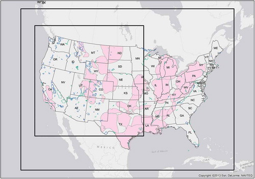
As shown in Figure 1, the model domain consists of a domain covering the entire continental United States with 36-km resolution grid cells, and a 12-km nested domain covered the western United States. Results presented in this document represent the inner 12-km domain only. Figure 1 also shows the locations of the national parks (outlined in blue) and other Class I areas (outlined in green), both of which are the focus of this analysis. While results are displayed for the entire 12-km domain, detailed results are presented for model grid cells where any part of the cell overlaps with the NP and Class I areas, as shown in Figure 1. Also shown in Figure 1 in pink are the extents of major oil and gas basins in the United States.

Figure 1. The CAMx modeling domain showing the outer 36-km domain covering the entire United States and the nested 12-km domain covering the western U.S. national parks, which are outlined in blue, and non-NPs Class I areas, which are in green. The extent of major U.S. oil and gas basins as of 2011 is shown in pink.

Source apportionment methods

For this photochemical modeling study, source apportionment techniques were used to estimate how emissions associated with oil and gas production and processing activity contributed to the concentration and deposition of air pollutants in national parks and Class I areas in the western United States. There are several tools within the CAMx modeling framework that are designed to facilitate the estimation of source contributions: ozone and particulate source apportionment tools (OSAT and PSAT, respectively), the direct decoupled method (DDM), and the brute force method (BFM).

The brute force method (BFM) was selected for this study. BFM estimates contributions of sources to air quality metrics by simply removing the emissions sources of interest one by one and rerunning the model to calculate the change in metrics due to the change in emissions from each source of interest. Because BFM requires an individual model run for each individual source group of interest, it can be time-intensive if multiple source groups are selected. However, the benefit of BFM is that all air quality metrics can be evaluated using a single run.

A BFM run was conducted in which all emissions associated with oil and gas production were removed from the emissions inventory and the model was rerun without them. The output was compared to a base case model run that included all emissions, and the difference in various air quality metrics represents the model estimated contribution of oil and gas to that metric.

Air quality metrics and thresholds

The source apportionment modeling provides estimates of the contribution of oil and gas emissions on air quality parameters most influenced by these emissions, including ozone, particulate matter, visibility, and nitrogen deposition in the national parks and elsewhere. These air quality parameters and associated metrics are of interest due to the negative impacts of these pollutants on human health, ecosystems, and visibility. For many of these air quality metrics, the impacts are evaluated by comparison to thresholds of concern. The modeling results are presented and interpreted within these known thresholds. The results presented in the paper are the absolute values of model output for each run, and the value of the difference between two model runs; monitor data are not incorporated into the results presented in this study.

Criteria pollutants

There are six pollutants, called criteria pollutants, for which the EPA has established NAAQS, thus setting limits for allowable ambient concentrations. The primary standards are set at levels considered protective of human health and the secondary standards are set at levels considered protective of human welfare (EPA, 2012). Human health impacts are a concern at national parks because of the amount of time visitors spend outside, often exerting themselves physically. While the primary NAAQS are designed to protect human health, air pollution can also cause damage to ecosystems. Protection of public welfare (including ecosystems) is considered when setting the secondary NAAQS. However, with the exception of annual PM_2.5 and short-term SO₂, the current secondary standards are identical to the primary standards. As described in the deposition, W126, and visibility sections in the following, the NAAQS may not be protective of sensitive ecosystems and resources.

Ozone

Ozone is known to cause negative human health impacts (Bell et al., 2004, 2005), as well as damage to ecosystems. For example, ground-level ozone has been linked to plant damage and decreases in crop yield (Kohut et al., 2012; Reilly et al., 2007). As of October, 2015, the primary ozone NAAQS is set at 70 parts per billion (ppb), and counties that do not meet this standard are EPA-designated “non-attainment” counties. The remaining areas are designated either as attainment areas, or “unclassifiable” where there is no regulatory monitor to demonstrate attainment. The secondary ozone standard is set equal to the primary standard.

The W126 ozone metric is a biologically relevant seasonal index commonly used to assess the impact of ozone on sensitive vegetation and ecosystems. The W126 metric quantifies cumulative daytime ozone exposure over the growing season in “parts per million-hours” (ppm-hr). The W126 is calculated by summing weighted hourly ozone from 8 a.m. to 8 p.m., and taking a 3-month running sum of exposure. W126 has been previously proposed as a secondary ozone standard in the range of 13 to 17 ppm-hr, with the maximum 3-month value averaged over 3 years. The NPS considers 7 ppm-hr to be the threshold above which effects begin in sensitive plant species and has recommended this level for the secondary standard (McCoy, 2015).

Particulate matter

Particulate matter with a diameter less than 2.5 µm (PM_2.5) is also known to cause negative impacts to human health (Krewski et al., 2009; Lepeule et al., 2012). Therefore, the NAAQS set the limits on 24-hr averaged and annually averaged concentrations of PM_2.5. Primary PM_2.5 standards are set at 35 µg/m³ and 12 µg/m³ for 24-hr averaged and annual values, respectively. The secondary annual PM_2.5 standard is set at 15 µg/m³, different from the primary standard.

Visibility

The 1977 Clean Air Act (CAA) amendments established the visibility protection provisions and declared in Section 169A “as a national goal the prevention of any future, and the remedying of any existing, impairment of visibility in mandatory class I Federal areas which impairment results from manmade air pollution.” Poor visibility can also increase people’s stress (Rotton and Frey, 1984) and cause changes in their activities and behaviors (Evans and Cohen, 1987). These negative effects are also recognized, and visibility in urban and other environments is protected by the 24-hr secondary particulate matter (PM) NAAQS, which is current set at the same level as the primary 24-hr PM standard.

To fulfill the CAA visibility requirements, the EPA promulgated the Regional Haze Rule (RHR) (EPA, 1999), which established the goal of returning visibility to natural conditions by the year 2064 in 156 Class I areas. Specifically, each state is to set reasonable progress goals to return visibility to natural conditions on the 20% haziest days by 2064, while maintaining visibility on the 20% clearest days (EPA, 2003). Haze levels are defined using the deciview (DV) index, calculated using eq 1 (Pitchford and Malm, 1994):

(1)

where b_ext is the light extinction due to gas and particles as estimated from speciated aerosol data measured in the Interagency Monitoring of Protected Visual Environments (IMPROVE) network (Hand et al., 2014). A change of 1 DV or more is considered noticeable under a number of limiting conditions (Pitchford and Malm, 1994). Under the EPA’s Best Available Retrofit Technology (BART) requirements, a source (if covered by BART) is identified as causing visibility impairment when modeling shows a contribution of one DV or more (EPA, 2004). When modeling shows that a covered source causes a change of 0.5 DV or more, that source is identified as contributing to visibility impairment under BART (EPA, 2004).

In order to be consistent with the RHR, 24-hr average modeled values consistent with the IMPROVE measurements were extracted for each model grid cell. Following the RHR procedures (EPA, 2003), 24-hr average light extinction and associated DV haze levels were calculated, from which the RHR haze tracking metrics, that is, the average DV of the 20% worst and best haze days, were estimated. Once the 20% best and worst haze days were determined for the base case, the same days were examined for the no oil and gas scenario case to determine the impact of oil and gas on visibility. Although IMPROVE operates on an every third day schedule, data from every model day were used in these analyses.

The assessment examines the contribution of oil and gas to the 20% best and worst haze days at each national park and other Class I areas. In addition, to better assess the impact to visitor experience, the number of modeled days with an average oil and gas impact greater than 0.5 DV and 1.0 DV were counted. With an average impact of 0.5 DV or more it is likely that oil and gas caused visible haze during some period of the day.

Nitrogen deposition

Reactive nitrogen deposition is a powerful fertilizer, and, in excess, fertilization (eutrophication) can cause changes in soil and water chemistry and acidification of soil and surface water, potentially resulting in changes in community structure, biodiversity, reproduction, and decomposition (Fenn et al., 1998). Long-term exposure of excess deposition may cause shifts in plant and animal species composition, increase in insect and disease outbreaks, and disruption of ecosystem processes such as nutrient cycling and wildfire frequency (Bobbink et al., 2010, 2003). Many lands in the western United States, such as the Rocky Mountain high alpine ecosystems, evolved with low levels of nitrogen deposition and are sensitive to a small increase in nitrogen deposition (Baron, 2006).

The critical load for a specific pollutant in a specific location is defined as “a quantitative estimate of the exposure to one or more pollutants below which significant harmful effects on specified sensitive elements of the environment do not occur according to preset knowledge” (Nilsson and Grennfelt, 1988, p.9). Evidence suggests that the critical load for nitrogen has been reached and exceeded in many regions throughout the United States (Pardo et al., 2011). Critical load values can put single-source contributions, like those from oil and gas production activities, into context by providing a target deposition level and allowing for comparison of estimated source contributions relative to that target value. The SI section B provides more information about estimated critical loads and about those loads related to total modeled nitrogen deposition.

Modeled total nitrogen includes model estimated annual wet and dry deposition totals for the following model species: reactive gaseous nitrogen, gaseous peroxy nitrogen, organic nitrates, gaseous nitric acid, particulate nitrate, gaseous ammonia (NH₃), and particulate ammonium (NH₄). Reactive gaseous nitrogen includes the nitrate radical (NO₃), nitrous acid (HONO), dinitrogen pentoxide (N₂O₅), and NO_x. The peroxys include peroxyl acetyl nitrate (PAN) and peroxy nitric acid (PNA). Organic nitrates modeled by CAMx include those that form from NO_y reactions with volatile organic compounds (VOCs), including isoprene, terpenes, xylene, toluene, and paraffins (Yarwood et al., 2005). Here, nitrogen, but not sulfur, deposition results are presented, because nitrogen is a much larger contributor to ecosystem effects (acidification and eutrophication) than is sulfur in the western United States.

Impacts of oil and gas production activity on air quality

Western United States

In general, model results show widespread contributions of oil and gas emissions to ozone, both daily maximum 8-hr average ozone and the ecology-based W126 ozone metric, and to total nitrogen deposition. The modeled contributions of oil and gas emissions to fine particulate matter (PM_2.5) and visibility are more localized, with modeled changes occurring within and near the major oil and gas basins.

National ambient air quality standards

Figure 2 presents the modeled contribution to the fourth highest daily maximum 8-hr ozone concentration for the entire 12-km domain in model year 2011. The model predicts widespread increases in the 4th highest daily maximum 8-hr ozone as a result of emissions associated with oil and gas activities.

Figure 2. Modeled contribution of emissions associated with oil and gas production activity to the fourth highest daily maximum 8-hr averaged ozone concentration in ppb. National parks and Class I areas are outlined in black.

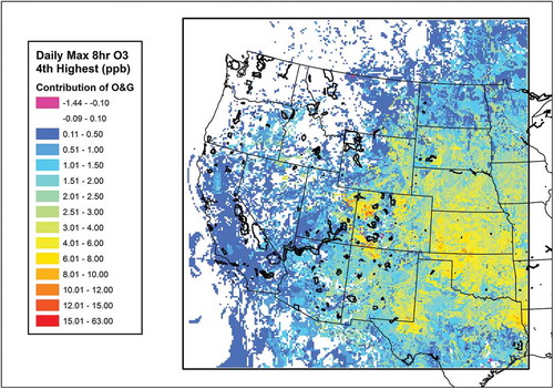
The maximum modeled contribution of oil and gas emissions to the fourth highest daily maximum 8-hr ozone concentration in Colorado, Utah, New Mexico, Kansas, and Oklahoma is between 10 and 15 ppb. The maximum contribution is 63 ppb in far eastern Texas. There are 24,624 square kilometers (171 12-km grid cells) where emissions associated with oil and gas production activity contribute >10% of the modeled fourth highest daily maximum 8-hr ozone concentration. SI section B presents additional results showing the contribution of oil and gas emissions to the daily maximum 8-hr ozone concentrations throughout the 12-km domain.

Modeled PM_2.5 impacts from oil and gas production activities, shown in Figure 3, are localized. Total PM_2.5 is the sum of many fine particulate species, including sulfate, nitrate, ammonium, organic carbon, elemental carbon, and soil. In the case of oil and gas, the largest changes are associated with fine soil and sulfate in the Intermountain West, and with nitrate in Texas. In the emissions inventory, fine soil emissions are primarily from site disturbance associated with the construction of well pads, roads, and pipelines, as well as transport operations associated with ongoing production activities. There is uncertainty associated with the speciation profiles used to assign both fine particulate matter (PM) and VOC emissions totals to the individual species in each respective category (fine PM and VOCs). In some areas, profiles and inventory assumptions may be updated and region specific, while others may not be. Emissions speciation is an ongoing topic for additional study, and the results presented here include the caveat of this uncertainty.

Figure 3. Modeled contribution of emissions associated with oil and gas production activity to annual average PM_2.5 concentration. National parks and Class I areas are outlined in black.

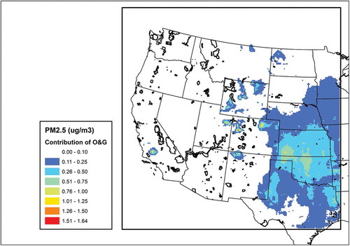
The largest modeled impact of oil and gas emissions to annually averaged PM_2.5 is 1.6 µg/m³ in northwestern New Mexico. There are 16 grid cells that show modeled oil and gas contributions >1 µg/m³, located in western Colorado, the Front Range in eastern Colorado, eastern Utah, central California, Wyoming, Oklahoma, Kansas, and northern New Mexico. There are 81,072 square kilometers (563 grid cells) with a modeled oil and gas contribution >0.5 µg/m³. There are 6,624 square kilometers (46 grid cells) with a modeled oil and gas contribution >10% of the base concentration.

Visibility

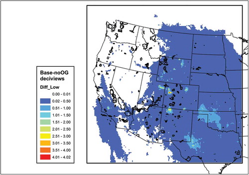
Because visibility impacts are driven by changes in PM_2.5 concentrations, the impacts of oil and gas activity on visibility are similar to impacts associated with PM_2.5. Modeled contributions of oil and gas emissions to visibility on the 20% worst and the 20% best days are shown in Figures 4 and 5, respectively. Visibility impacts are localized and are dominated by elemental and organic carbon in Colorado, Wyoming, Utah, and New Mexico. Changes in visibility due to the formation of nitrate from oil and gas emissions are widespread in Texas, Oklahoma, and Nebraska, especially in the winter. Overall, there are 273,600 square kilometers (1900 grid cells) with an annual average impact to visibility greater than 0.5 DV.

Figure 4. Modeled contribution of emissions associated with oil and gas production activity to visibility on the 20% haziest days. National parks and Class I areas are outlined in black.

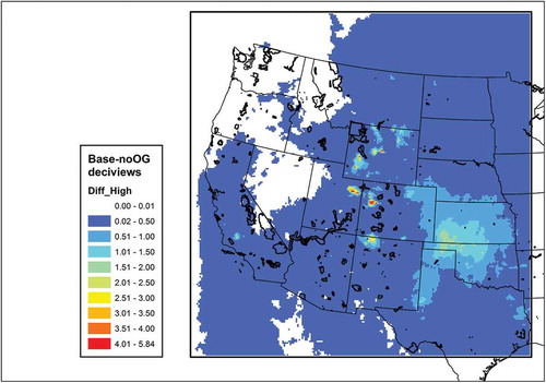
Figure 5. Modeled contribution of emissions associated with oil and gas production activity to visibility on the 20% clearest days. National parks and Class I areas are outlined in black.

Ecological effects

Air quality can impact the health of ecosystems in many ways. Here, metrics related to two air quality/ecosystem interactions are presented in the context of how emissions of oil and gas production activity contribute to each metric: total nitrogen deposition and W126 ozone.

Figure 6 shows the modeled contribution of emissions associated with oil and gas production activity to total annual nitrogen deposition. Nitrogen impacts are widespread, with the largest impacts occurring near areas of intense oil and gas production.

Figure 6. Modeled contribution of emissions associated with oil and gas production activity to total nitrogen deposition (kg N/ha/year). National parks and Class I areas are outlined in black.

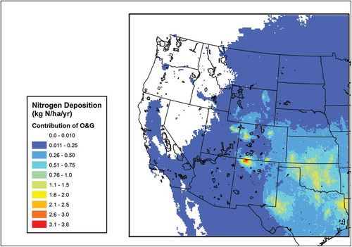
There are 70,272 square kilometers (488 12-km cells) with a modeled contribution of oil and gas emissions to total nitrogen deposition >1 kg N/ha/yr. There are 17,568 square kilometers (122 12-km cells) with a modeled contribution of oil and gas emissions to total nitrogen deposition >30% of base total (84,240 km² with >20%, 493,488 km² with >10%). There are 145,584 square kilometers (1011 cells) where modeling suggests that oil and gas emissions pushed total nitrogen deposition above the most conservative critical load associated with the ecosystem in that grid cell.

Ozone concentrations can also impact the health of sensitive vegetation and ecosystems. The impacts of emissions associated with oil and gas production activity, to the maximum 3-month W126 metric (the maximum 3-month W126 typically occurs in summer due to increased photochemistry and biogenic VOC emissions associated with summer meteorology), is presented here. Model output (as shown in Figure 7) shows widespread increases in W126 due to oil and gas, with an average increase across the U.S. land area that falls within the 12-km modeling domain of 2.1 ppm-hr.

Figure 7. Modeled contribution of emissions associated with oil and gas production activity to the annual maximum W126 ozone concentration (ppm-hr). National parks and Class I areas are outlined in black.

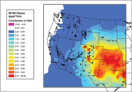
The maximum modeled contribution of oil and gas emissions to W126 ozone is 55 ppm-hr in Texas. The model results show widespread increases in W126 ozone greater than 5 ppm-hr over northern Texas, Oklahoma and Kansas, Colorado, and New Mexico. There are 474,912 square kilometers (3298 cells) where the model suggests oil and gas contribute >20% of total modeled W126 values (2,156,544 km² with >10%).

National parks and non-NPS-Class I areas

There are 162 total national parks and 66 U.S. Fish & Wildlife Service or U.S. Forest Service Class I areas in the 12-km domain (referred to generally as “units” in this report). In this section of the report, results of the modeling study are reported for grid cells that overlap any size area within the boundaries of those National Parks and Class I areas. Unless otherwise specified, the values reported are for the grid cell with the highest modeled contribution from oil and gas emissions in each of the units of interest. For each air quality metric in the following, the 20 national parks and Class I areas with the largest impact from oil and gas emissions are presented. SI section C contains each of the tables cited here, for all National Parks and Class I areas in the 12-km domain.

Ozone: 8 hr & W126

The results for the contribution of oil and gas emission to the fourth highest daily maximum 8-hr ozone concentration are presented in Table 1 in the main paper, and Tables C3 and C4 in the Supplemental Information. There are 88 units where the maximum contribution of oil and gas emissions to the fourth highest 8-hr ozone concentration is greater than 2 ppb in at least one grid cell. There are 139 units with an oil and gas contribution to the fourth highest 8-hr ozone concentration greater than 1 ppb. The largest contribution occurred at Washita Battlefield at 7 ppb.

Table 1. Twenty national parks and Class I areas with the largest contribution of oil and gas emissions to the fourth highest daily maximum 8-hr ozone concentration (ppb).

NPS unit	State	Name	Base case (ppb)	No oil and gas (ppb)	Oil and gas contribution (ppb)	Percent of base case
Yes	OK	Washita Battlefield	76.3	69.3	7.0	9.2%
Yes	UT	Hovenweep	78.0	71.4	6.6	8.5%
Yes	CO	Dinosaur	73.6	67.2	6.4	8.7%
	CO	Weminuche Wilderness	81.3	74.9	6.4	7.9%
Yes	KS	Fort Larned	75.2	68.9	6.3	8.4%
	CO	Flat Tops Wilderness	72.2	66.4	5.7	8.0%
Yes	MO	Harry S. Truman	88.9	83.3	5.6	6.3%
Yes	KS	Fort Scott	78.3	72.8	5.5	7.0%
Yes	NM	Aztec Ruins	82.5	77.2	5.3	6.4%
Yes	NM	Pecos Wilderness	82.8	77.6	5.2	6.3%
Yes	CO	Colorado	73.3	68.2	5.2	7.1%
Yes	CO	Rocky Mountain	73.1	68.2	4.9	6.7%
Yes	MO	George Washington Carver	85.1	80.4	4.7	5.6%
Yes	UT	Arches	75.0	70.2	4.7	6.3%
Yes	AR	Pea Ridge	80.7	76.6	4.2	5.2%
	CO	Maroon Bells–Snowmass Wilderness	74.3	70.3	4.0	5.4%
	AR	Caney Creek Wilderness	74.7	70.8	3.9	5.2%
Yes	AR	President William Jefferson Clinton Birthplace Home	77.4	73.6	3.8	5.0%
Yes	CO	Bent’s Old Fort	74.7	70.9	3.8	5.0%
	CO	Mount Zirkel Wilderness	73.1	69.4	3.7	5.0%

As shown in Table 2 in the main paper, and Tables C5 and C6 in the Supplemental Information, 68 NPs and other Class I areas in the 12-km modeling domain contain at least one grid cell where the modeled oil and gas emissions contribute more than 10% of the base case W126 metric. Ninety-five units had a maximum contribution of more than 1 ppm-hr.

Table 2. Twenty national parks and Class I areas with the largest contribution of oil and gas emissions to the W126 ozone metric (ppm-hr).

NPS unit	State	Park name	Base case W126	No oil and gas W126	Difference W126	Percent of base case
Yes	KS	Fort Larned	30.35	21.97	8.37	28%
Yes	OK	Washita Battlefield	31.86	24.03	7.82	25%
Yes	AR	President William Jefferson Clinton Birthplace Home	32.46	25.25	7.21	22%
Yes	AR	Fort Smith	35.74	28.71	7.02	20%
Yes	OK	Chickasaw	40.84	33.94	6.90	17%
Yes	KS	Tallgrass Prairie	31.62	24.84	6.78	21%
Yes	CO	Dinosaur	24.42	17.89	6.53	27%
Yes	CO	Sand Creek Massacre	29.47	23.06	6.41	22%
Yes	KS	Nicodemus	23.65	17.58	6.07	26%
Yes	TX	Lake Meredith	38.68	32.63	6.05	16%
Yes	KS	Brown v. Board of Education	36.88	30.84	6.04	16%
	CO	Flat Tops Wilderness	24.25	18.39	5.86	24%
Yes	TX	Alibates Flint Quarries	38.55	32.79	5.76	15%
Yes	AR	Buffalo	26.58	20.99	5.60	21%
	AR	Upper Buffalo Wilderness	26.58	20.99	5.60	21%
Yes	CO	Bent’s Old Fort	28.63	23.05	5.58	20%
Yes	KS	Fort Scott	31.71	26.15	5.56	18%
Yes	AR	Pea Ridge	33.52	28.19	5.33	16%
Yes	NM	Carlsbad Caverns NP	29.47	24.22	5.24	18%
	CO	Weminuche Wilderness	27.73	22.62	5.11	18%

Visibility

The impact of oil and gas on visibility in NPs and Class I areas is presented in Table 3. Modeling results suggest that oil and gas significantly degrades visibility at a number of Class I and II national parks and Class I wilderness areas near oil and gas fields. At 11 Class II national parks, which are not subject to the Regional Haze Rule requirements, the oil and gas production activity contributed more than 0.5 DV to the average 20% worst haze days. In addition, at 36 NPs and Class I areas, oil and gas caused more than 0.5 DV of haze on more than 20 days per year. At Aztec Ruins nearly every day of the year had contributions greater than 0.5 DV. This indicates the potential for the regular occurrence of visible haze degrading the visitor’s experience.

Table 3. Twenty national parks and Class I areas with the largest contribution of oil and gas emissions to the average visibility index ranked by the impact on the 20% haziest days (dv), and the number of days the modeled oil and gas impact to visibility is greater than 0.5 dv and 1.0 dv.

NPS unit	Park name	State	Oil and gas Avg Impacts on 20% haziest days (dv)	Oil and gas average impacts on 20% clearest days (dv)	Number of days average impacts >0.5 dv	Number of days average impacts >1.0 dv
Yes	Fort Larned	KS	1.18	0.29	132	78
Yes	Lake Meredith	TX	0.91	0.55	147	65
Yes	Colorado	CO	0.88	0.31	85	24
Yes	Sand Creek Massacre	CO	0.84	0.20	105	39
Yes	Aztec Ruins	NM	0.81	0.84	323	127
Yes	Alibates Flint Quarries	TX	0.81	0.54	136	57
Yes	Homestead	NE	0.79	1.11	279	162
Yes	Tallgrass Prairie	KS	0.70	0.19	84	25
Yes	Nicodemus	KS	0.67	0.16	85	34
Yes	Washita Battlefield	OK	0.65	0.72	187	82
Yes	Dinosaur	CO	0.61	0.28	107	22
Yes	Bent’s Old Fort	CO	0.49	0.09	40	11
Yes	Fort Scott	KS	0.46	0.18	55	17
Yes	Fort Smith	AR	0.45	0.21	61	10
Yes	Fort Laramie	WY	0.43	0.09	28	1
Yes	Bighorn Canyon	MT	0.43	0.13	37	10
Yes	Scotts Bluff	NE	0.41	0.10	41	1
Yes	Brown v. Board of Education	KS	0.39	0.07	30	8
Yes	Pea Ridge	AR	0.39	0.16	50	4
Yes	Devils Tower	WY	0.39	0.07	33	2

Nitrogen deposition and critical loads results

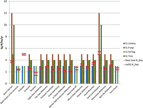
There are 26 units in the 12-km domain that contain at least one grid cell showing that modeled contribution of oil and gas emissions push the modeled total nitrogen deposition from below the CL to above the CL. Table 4 shows the 20 national parks or Class I areas with the largest modeled contribution from oil and gas to total nitrogen deposition. Figure 8 shows total nitrogen deposition for both the base case model run and the run without oil and gas emissions along with the lower range critical load values for four different end points, for all Class I and II units in Colorado.

Table 4. Twenty national parks and Class I areas with the largest contribution of oil and gas emissions to total nitrogen deposition (Ndep).

NPS unit	State	Park name	Base Ndep (kg N/ha/yr)	No oil and gas Ndep	Maximum difference	Percent of base total	Most conservative critical load value
Yes	NM	Aztec Ruins	5.79	3.88	1.91	32.9%	3
Yes	NE	Homestead	12.30	10.95	1.35	11.0%	5
Yes	OK	Washita Battlefield	5.63	4.75	0.88	15.6%	5
Yes	OK	Chickasaw	10.31	9.45	0.86	8.4%	5
Yes	AR	Fort Smith	24.22	23.36	0.86	3.5%	3
Yes	TX	Big Thicket	7.72	6.95	0.77	9.9%	3
Yes	TX	San Antonio Missions	20.31	19.58	0.74	3.6%	5
Yes	TX	Lake Meredith	7.07	6.44	0.63	8.9%	5
	AR	Caney Creek Wilderness	11.08	10.46	0.62	5.6%	3
Yes	KS	Brown v. Board of Education	15.56	14.94	0.62	4.0%	5
Yes	TX	Alibates Flint Quarries	8.14	7.53	0.61	7.4%	5
Yes	KS	Fort Larned	8.63	8.07	0.56	6.5%	5
Yes	MO	Harry S Truman	17.68	17.13	0.56	3.2%	5
Yes	AR	President William Jefferson Clinton Birthplace Home	13.88	13.35	0.53	3.8%	3
Yes	KS	Tallgrass Prairie	8.38	7.85	0.53	6.3%	5
	CO	Weminuche Wilderness	2.53	2.00	0.53	20.8%	2
Yes	CO	Dinosaur	1.92	1.41	0.51	26.4%	3
	CO	Flat Tops Wilderness	2.86	2.36	0.51	17.7%	2
Yes	AR	Buffalo	10.04	9.54	0.50	5.0%	3
	AR	Upper Buffalo Wilderness	10.04	9.54	0.50	5.0%	3

Figure 8. Colorado national parks and Class I areas showing total modeled nitrogen deposition results both with (lighter red horizontal bar) and without (darker red horizontal bar) oil and gas emissions, plus the lower range critical load values for four endpoints (vertical bars).

Discussion

While the emissions inventories used in this study represent the best available data for the western United States, there remains a great deal of uncertainty with respect to these emissions. Measurement studies along the Colorado Front Range, for example, suggest that inventories of VOC emissions from oil and gas are underestimated in that region by 50% to 300%, depending on the species (Gilman et al., 2013; Petron et al., 2012; Swarthout et al., 2013). Additionally, there are several potential categories of emissions sources that are not included in oil and gas inventories because there are not enough data to estimate emissions. These “missing” sources include production water evaporation ponds, field gathering pipelines, and nonroutine events including pipeline blowdowns, spills, upsets, and maintenance activities. Additionally, on-road mobile sources (trucking) associated with oil and gas production are likely underestimated, and are included in the on-road inventory, not in the oil and gas inventory, so their impacts are not included in this analysis.

Another potentially large source of uncertainty with respect to emissions inventories is the concept of skewed sources, either from high-emitting processes or from poorly performing sources with much higher emissions than average (Allen, 2014). An example of a high-emitting process would be the venting of VOCs in a liquids unloading procedure. Poorly performing sources may be leaking or malfunctioning, or they may be much older with different emissions standards. Emissions totals from these sources are much larger than those calculated using the “average” emissions factors typically used for emissions inventories, and as a result, representative or “average” emissions inventories may be underestimated. For example, a recent study measured emissions from pneumatic controllers on wells throughout the United States, finding that a subset of the highest emitting controllers (less than 20% of the total) emitted more than 95% of the total emissions from controllers (Allen et al., 2015).

It was noted that the analysis presented here includes impacts associated with oil and gas emissions only. The air quality impacts of many emissions associated with processing, transportation, and delivery of oil and gas and its products are not included here. As natural gas is processed, impurities and heavier hydrocarbons are removed, leaving a product that is mostly methane. Therefore, any leaks or other fugitive emissions of natural gas after processing are less likely to contain heavier and more reactive hydrocarbons. However, equipment associated with oil and gas processing and compression can be large sources of nitrogen oxides (UNC and ENVIRON, 2014). Additionally, previously rural areas, where large oil and gas development occurs, can experience population growth as people move to the area to work on oil and gas fields. As population increases, emissions associated with private transportation, home heating, support businesses (dry cleaners, water treatment plants, etc.), and many other sources of emissions also increase.

Measurement data in conjunction with the inventory data in Colorado indicate that, despite estimated per-well emissions decreases, total VOC emissions from oil and gas have increased over the last 10 years (Colorado Department of Public Health and Environment [CDPHE], 2008; Swarthout et al., 2013; Bar-Ilan et al., 2013). It is possible that this trend could continue if the growth of the industry continues on a similar path, thus suggesting that emissions from oil and gas activity could become a larger source of air pollution to national parks in the future. However, increasing regulatory efforts with respect to the oil and gas sector (and changing prices) could produce different trends in different parts of the country.

Finally, despite this study including a full year of modeling results, the impacts presented in this report do not include the relatively new phenomenon of high wintertime ozone events over oil and gas fields. In Utah’s Uintah Basin and in Wyoming’s Upper Green River Basin, activity associated with oil and gas production has been identified as the cause for wintertime ozone nonattainment events in those areas (Schnell et al., 2009; Lyman and Shorthill, 2013; Edwards et al., 2014). However, much is still unknown about the chemical and physical processes that cause wintertime ozone (Ahmadov et al., 2015; Koss et al., 2015). As a result, a sound theoretical underpinning for wintertime ozone formation is not yet available to effectively model this phenomenon and therefore the potential impacts of wintertime emissions are not included here.

Conclusion

Modeling results suggest that the emissions associated with oil and gas production activity are having a negative impact on the air quality and ecosystem health in our National Parks and Class I areas. Results show 139 units in the western United States where oil and gas emissions contribute ≥1 ppb to the modeled fourth highest daily maximum 8-hr ozone concentration in at least one grid cell located in that unit. Similarly, there are 68 units with an oil and gas contribution greater than 1 ppm-hr to the modeled ozone W126 values. There are 26 units in the western United States where oil and gas emissions push the modeled total nitrogen deposition above the most conservative value of the critical load for that particular unit (without oil and gas emissions, the modeled total nitrogen deposition would be below the critical load value in those units). In both cases, these results suggest that oil and gas emissions are causing, or contributing to, a violation of health standards and air quality related values threshold exceedances, and thus potentially harming ecosystems and affecting visitor health in these units. In addition, oil and gas activity appears to be regularly causing visible haze in national parks units near the development. While there is still a great deal of uncertainty associated with oil and gas emissions, this analysis suggests that oil and gas emissions inventories are underestimated. Despite likely being underestimated, these oil and gas emissions are still a significant source of pollution in national parks and Class I areas.

Acknowledgment

The data used in this study are from a regional photochemical modeling platform hosted by the Intermountain West Data Warehouse (IWDW) and prepared under the associated Western Air Quality Study (WAQS) as noted in the References section of this paper. The IWDW holds and manages all original and derivative files prepared under the IWDW-WAQS for the purposes of its cooperator/sponsor agencies, using publicly available protocols and procedures. The IWDW-WAQS manages access to and use of those data as proprietary. Documentation as described on the IWDW website is required prior to the transfer or alternate subsequent application of any requested data. The data used in this study were requested from the IWDW-WAQS and provided as authorized for the National Park Service’s Grand Teton Reactive Nitrogen Deposition Study (GrandTRENDS). The data used in this study were then repurposed for the analysis reported in this paper, which is beyond the scope of the original GrandTRENDS project, and is not a IWDW-WAQS cooperator/sponsor agencies’ prior-authorized application of their modeling platform. The scientific veracity of this study and analysis reported in this paper have been subjected to peer review, including by representatives of the IWDW-WAQS. For more information about access to and use of IWDW-WAQS modeling platform data, contact Tom Moore ([email protected]).

Funding

This work was funded by the National Park Service under cooperative agreement P14AC00728. The assumptions, findings, conclusions, judgments, and views presented herein are those of the authors and should not be interpreted as necessarily representing the National Park Service.

Supplemental data

Supplemental data for this article can be accessed on the publisher’s website.

Additional information

Funding

This work was funded by the National Park Service under cooperative agreement P14AC00728. The assumptions, findings, conclusions, judgments, and views presented herein are those of the authors and should not be interpreted as necessarily representing the National Park Service.

Notes on contributors

Tammy M. Thompson

Tammy M. Thompson is currently a Science and Technology Policy Fellow with the American Association for the Advancement of Science in Washington DC. At the time this research was conducted and accepted for publication, Dr. Thompson was working as a Research Scientist II at the Cooperative Institute for Research of the Atmosphere (CIRA) at Colorado State University in Fort Collins, CO.

Donald Shepherd

Donald Shepherd is an environmental engineer with the Air Resource Division of the National Park Service in Lakewood, CO.

Andrea Stacy

Andrea Stacy is an environmental protection specialist with the Air Resource Division of the National Park Service in Lakewood, CO.

Michael G. Barna

Michael G. Barna is a physical scientist with the Air Resource Division of the National Park Service in Fort Collins, CO.

Bret A. Schichtel

Bret A. Schichtel is a research physical scientist with the Air Resource Division of the National Park Service in Fort Collins, CO.

References

- Abt Associates Inc. 2012. BenMAP, Environmental Benefits Mapping and Analysis Program. User’s Manual, Version 4.0. EPA Office of Air Quality Planning and Standards. http://www.epa.gov/airquality/benmap/docs.html ( accessed July 2013).
- Adelman, Z., and B.H. Baek. 2015. Three-state air quality modeling study emissions modeling report, Simulation years 2008 and 2011. http://vibe.cira.colostate.edu/wiki/Attachments/Emissions/3SAQS_Emissions_Modeling_Report_v18Feb2015_Final.pdf
- Adelman, Z., U. Shankar, D. Yang, and R. Morris. 2015. Three-state air quality modeling study CAMx photochemical grid model, Model performance evaluation, Simulation year 2011. http://vibe.cira.colostate.edu/wiki/Attachments/Modeling/3SAQS_Base11a_MPE_Final_18Jun2015.pdf.
- Ahmadov, R., S. McKeen, M. Trainer, R. Banta, A. Brewer, S. Brown, P.M. Edwards, J.A. de Gouw, G.J. Frost, J. Gilman, and D. Helmig. 2015. Understanding high wintertime ozone pollution events in an oil- and natural gas-producing region of the western US. Atmos. Chem. Phys. 15:411–29.
- Allen, D.T. 2014. Methane emissions from natural gas production and use: reconciling bottom-up and top-down measurements. Curr. Opin. Chem. Eng, Energy Environ. Eng./Reaction Eng. 5:78–83. doi:10.1016/j.coche.2014.05.004.
- Allen, D.T., A.P. Pacsi, D.W. Sullivan, D. Zavala-Araiza, M. Harrison, K. Keen, M.P. Fraser, A.D. Hill, R.F. Sawyer, and J.H. Seinfeld. 2015. Methane emissions from process equipment at natural gas production sites in the United States: Pneumatic controllers. Environ. Sci. Technol. 49:633–40. doi:10.1021/es5040156
- Bar-Ilan, A., and T. Moore. 2013. Upstream oil and gas emissions inventories: Regulatory and technical considerations. Presentation at Air Quality and Oil & Gas Development in the Rocky Mountain Region, Boulder, CO, October 21. http://www.wrapair2.org/pdf/Moore_Barilan_OandG_Inventories_10_20_13.pdf
- Baron, J.S. 2006. Hindcasting nitrogen deposition to determine an ecological critical load. Ecol. Appl. 16:433–39. doi:10.1890/1051-0761(2006)016[0433:HNDTDA]2.0.CO;2.
- Bell, M.L., F. Dominici, and J.M. Samet. 2005. A meta-analysis of time-series studies of ozone and mortality with comparison to the National Morbidity, Mortality, and Air Pollution Study. Epidemiology 16:436–45. doi:10.1097/01.ede.0000165817.40152.85
- Bell, M.L., A. McDermott, S.L. Zeger, J.M. Samet, and F. Dominici. 2004. Ozone and short-term mortality in 95 US urban communities, 1987–2000. J. Am. Med. Assoc. 292:2372–78. doi:10.1001/jama.292.19.2372
- Bobbink, R., M. Ashmore, S. Braun, W. Flückiger, and I.J. Van den Wyngaert. 2003. Empirical nitrogen critical loads for natural and semi-natural ecosystems: 2002 Update. In Empirical Critical Loads for Nitrogen, 43–170. http://www.iap.ch/en/publikationen/nworkshop-background.pdf (accessed February 3, 2017).
- Bobbink, R., K. Hicks, J. Galloway, T. Spranger, R. Alkemade, M. Ashmore, M. Bustamante, S. Cinderby, E. Davidson, F. Dentener, B. Emmett, J.-W. Erisman, M. Fenn, F. Gilliam, A. Nordin, L. Pardo, and W. De Vries. 2010. Global assessment of nitrogen deposition effects on terrestrial plant diversity: A synthesis. Ecol. Appl. 20:30–59. doi:10.1890/08-1140.1.
- Colorado Department of Public Health and Environment et al. 2008. Denver Metropolitan Area and North Front Range 8-hour ozone State Implementation Plan: Emissions inventory. http://www.colorado.gov/airquality/documents/deno308/Emission_Inventory_TSD_DraftFinal.pdf.
- Edwards, P.M., S.S. Brown, J.M. Roberts, R. Ahmadov, R.M. Banta, W.P. Dubé, R.A. Field, J.H. Flynn, J.B. Gilman, M. Graus, and D. Helmig. 2014. High winter ozone pollution from carbonyl photolysis in an oil and gas basin. Nature 514:351–54. doi:10.1038/nature13767
- Energy Information Administration. 2014a. Short term energy outlook, August 12, 2014. http://www.eia.gov/forecasts/steo/index.cfm
- Energy Information Administration, 2014b. Annual energy outlook, early release. http://www.eia.gov/forecasts/aeo/er/index.cfm
- Energy Information Administration, 2013. Natural gas summary, Colorado: Number of producing gas wells. www.eia.gov/dnav/ng/ng_sum_lsum_dcu_SCO_a.htm
- ENVIRON. 2015. User’s guide: Comprehensive Air Quality Model with Extensions, version 6.2. ENVIRON International Corporation. http://www.camx.com ( accessed January 2016).
- Environmental Protection Agency. 1999. 40 CFR Part 51—Regional haze regulations: Final rule. Fed. Reg. 64(126): 35714–774.
- Environmental Protection Agency, 2003. Guidance for tracking progress under the regional haze rule, contract no. 68-D-02-0261. http://www.epa.gov/ttnamti1/files/ambient/visible/tracking.pdf
- Environmental Protection Agency. 2004. 40 CFR Part 51—Regional haze regulations and guidelines for best available retrofit technology (BART) determinations. Fed. Reg. 69(87): 25184–232. https://www.gpo.gov/fdsys/pkg/FR-2004-05-05/pdf/04-9863.pdf
- Environmental Protection Agency. 2007. Guidance on the use of models and other analyses for demonstrating attainment of air quality goals for ozone, PM2.5, and regional haze. Office of Air Quality Planning and Standards. http://www.epa.gov/scram001/guidance/guide/final-03-pm-rh-guidance.pdf.
- Environmental Protection Agency. 2012. National ambient air quality standards, Office of Air Quality Planning and Standards. http://www.epa.gov/air/criteria.html
- Environmental Protection Agency. 2013. Office of Inspector General (OIG) report, EPA needs to improve air emissions data for the oil and natural gas production sector. Report 13-P-0161. https://www.epa.gov/sites/production/files/2015-09/documents/20130220-13-p-0161.pdf (accessed February 3, 2017).
- Environmental Protection Agency. 2015a. 2011 National emissions inventory, version 2, Technical support document, Office of Air and Radiation. https://www.epa.gov/air-emissions-inventories/2011-national-emissions-inventory-nei-documentation
- Environmental Protection Agency. 2015b. National ambient air quality standards for ozone. Final rule EPA-HQ-OAR-2008-0699; FRL-9918-43-OAR. Office of Air Quality Planning and Standards. http://www3.epa.gov/ozonepollution/pdfs/20151001fr.pdf
- Environmental Protection Agency. 2015c. Emission standards for new and modified sources, 80 FR 56593. http://www3.epa.gov/airquality/oilandgas/basic.html
- Evans, G.W., and S. Cohen. 1987. Environmental stress. In Handbook of Environmental Psychology, ed. D. Stokols and I. Altman, 571–610. New York, NY: John Wiley and Sons.
- Fenn, M.E., M.A. Poth, J.D. Aber, J.S. Baron, B.T. Bormann, D.W. Johnson, A.D. Lemly, S.G. McNulty, D.F. Ryan, and R. Stottlemyer. 1998. Nitrogen excess in North American ecosystems: Predisposing factors, ecosystem responses, and management strategies. Ecol. Appl. 8:706–33. doi:10.1890/1051-0761(1998)008[0706:NEINAE]2.0.CO;2.doi:10.1890/1051-0761(1998)008[0706:NEINAE]2.0.CO;2
- Gilman, J.B., B.M. Lerner, W.C. Kuster, and J.A. de Gouw. 2013. Source signature of volatile organic compounds from oil and natural gas operations in northeastern Colorado. Environ. Sci. Technol. 47:1297–305. doi:10.1021/es304119a
- Hand, J.L., B.A. Schichtel, W.C. Malm, S. Copeland, J.V. Molenar, N. Frank, and M. Pitchford. 2014. Widespread reductions in haze across the United States from the early 1990s through 2011. Atmos. Environ. 94:671–79. doi:10.1016/j.atmosenv.2014.05.062
- Huang, Y., F. Dominici, and M.L. Bell. 2005. Bayesian hierarchical distributed lag models for summer ozone exposure and cardio-respiratory mortality. Environmetrics 16:547–62. doi:10.1002/(ISSN)1099-095X
- Intermountain West Data Warehouse–Western Air Quality Study. 2016. AQS Modeling Platform 2011a. http://views.cira.colostate.edu/tsdw ( accessed August 2015).
- Ito, K., S.F. De Leon, and M. Lippmann. 2005. Associations between ozone and daily mortality: Analysis and meta-analysis. Epidemiology 16:446–57. doi:10.1097/01.ede.0000165821.90114.7f
- Kohut, R., C. Flanagan, J. Cheatham, and E. Porter. 2012. Foliar ozone injury on cutleaf coneflower at Rocky Mountain National Park, Colorado. West. North Am. Nat. 72:32–42. doi:10.3398/064.072.0104
- Koo, B., G.M. Wilson, R.E. Morris, A.M. Dunker, and G. Yarwood. 2009. Comparison of source apportionment and sensitivity analysis in a particulate matter air quality model. Environ. Sci. Technol. 43:6669–75. doi:10.1021/es9008129
- Koss, A.R., J. de Gouw, C. Warneke, J.B. Gilman, B.M. Lerner, M. Graus, B. Yuan, P. Edwards, S.S. Brown, R. Wild, and J.M. Roberts. 2015. Photochemical aging of volatile organic compounds associated with oil and natural gas extraction in the Uintah Basin, UT, during a wintertime ozone formation event. Atmos. Chem. Phys. Discuss. 15:6403–44. doi:10.5194/acpd-15-6403-2015
- Krewski, D., M. Jerrett, R.T. Burnett, R. Ma, E. Hughes, Y. Shi, M.C. Turner, C.A. Pope III, G. Thurston, E.E. Calle, and M.J. Thun. 2009. Extended follow-up and spatial analysis of the American Cancer Society study linking particulate air pollution and mortality. Res. Rep. Health Effects Inst. 5:114; discussion 115–36.
- Lepeule, J., F. Laden, D. Dockery, and J. Schwartz. 2012. Chronic exposure to fine particles and mortality: An extended follow-up of the Harvard Six Cities Study from 1974 to 2009. Environ. Health Perspect. 120:965–70. doi:10.1289/ehp.1104660
- Levy, J.I., S.M. Chemerynski, and J.A. Sarnat. 2005. Ozone exposure and mortality: An empiric Bayes metaregression analysis. Epidemiology 16:458–68. doi:10.1097/01.ede.0000165820.08301.b3
- Lyman, S., and H. Shorthill. 2013. Final report: 2012 Uintah Basin winter ozone & air quality study. Doc. no. CRD13-320.32, Commercialization and Regional Development, Utah State University. http://rd.usu.edu/files/uploads/ubos_2011-12_final_report.pdf.
- McCoy, C. 2015. Comments to “Environmental Protection Agency’s Proposal to Revise the National Ambient Air Quality Standards for Ozone.” Letter to Erika Sasser. April 14. National Park Service, Air Resources Division. https://www.regulations.gov/document?D=EPA-HQ-OAR-2008-0699-3871 (accessed February 3, 2017).
- Nilsson, J., and P. Grennfelt. 1988. Critical loads for sulphur and nitrogen: Report from a workshop held at Skokloster, Sweden, 19–24 March, 1988. Nordic Council of Ministers. https://hero.epa.gov/hero/index.cfm/reference/details/reference_id/36242 (accessed February 3, 2017).
- Pardo, L.H., M.E. Fenn, C.L. Goodale, L.H. Geiser, C.T. Driscoll, E.B. Allen, J.S. Baron, R. Bobbink, W.D. Bowman, C.M. Clark, and B. Emmett. 2011. Effects of nitrogen deposition and empirical nitrogen critical loads for ecoregions of the United States. Ecol. Appl. 21:3049–82. doi:10.1890/10-2341.1
- Pétron, G. G. Frost, B.R. Miller, A.I. Hirsch, S.A. Montzka, A. Karion, M. Trainer, C. Sweeney, A.E. Andrews, L. Miller, and J. Kofler. 2012. Hydrocarbon emissions characterization in the Colorado Front Range: A pilot study. J. Geophys. Res. 117:D04304.
- Pitchford, M.L., and W.C. Malm. 1994. Development and applications of a standard visual index. Atmos. Environ. 28(5): 1049–54. doi:10.1016/1352-2310(94)90264-X
- Prenni, A.J., D.E. Day, A.R. Evanoski-Cole, B.C. Sive, A. Hecobian, Y. Zhou, K.A. Gebhart, J.L. Hand, A.P. Sullivan, Y. Li, M.I. Schurman, Y. Desyaterik, W.C. Malm, J.L. Collett, Jr., and B.A. Schichtel. 2016. Oil and gas impacts on air quality in federal lands in the Bakken region: An Overview of the Bakken Air Quality Study and first results. Atmos. Chem. Phys. 16:1401–16. doi:10.5194/acp-16-1401-2016.
- Regional Air Quality Council. 2016. Moderate area ozone SIP for the Denver Metro and North Front Range nonattainment area. https://raqc.egnyte.com/dl/geyEqNjlla/FinalProposedModerateOzoneSIP_2016-07-07.pdf.
- Reilly, J., S. Paltsev, B. Felzer, X. Wang, D. Kicklighter, J. Melillo, R. Prinn, M. Sarofim, A. Sokolov, and C. Wang. 2007. Global economic effects of changes in crops, pasture, and forests due to changing climate, carbon dioxide, and ozone. Energy Policy 35:5370–83. doi:10.1016/j.enpol.2006.01.040
- Rodriguez, M.A., M.G. Barna, and T. Moore. 2009. Regional impacts of oil and gas development on ozone formation in the western United States. J. Air Waste Manage. Assoc. 59:1111–18. doi:10.3155/1047-3289.59.9.1111
- Rotton, J., and J. Frey. 1984. Psychological costs of air pollution: Atmospheric conditions, seasonal trends, and psychiatric emergencies. J. Popul. Environ. 7(1):3–16. doi:10.1007/BF01257469
- Schnell, R.C., S.J. Oltmans, R.R. Neely, M.S. Endres, J.V. Molenar, and A.B. White. 2009. Rapid photochemical production of ozone at high concentrations in a rural site during winter. Nat. Geosci. 2:120–22. doi:10.1038/ngeo415
- Schwartz, J. 2005. How sensitive is the association between ozone and daily deaths to control for temperature? Am. J. Respir. Crit. Care Med. 171:627–31. doi:10.1164/rccm.200407-933OC
- Swarthout, R.F., R.S. Russo, Y. Zhou, A.H. Hart, and B.C. Sive. 2013. Volatile organic compound distributions during the NACHTT campaign at the Boulder Atmospheric Observatory: Influence of urban and natural gas sources. J. Geophys. Res. Atmos. 118:10,614–37. doi:10.1002/jgrd.50722
- University of North Carolina and ENVIRON. 2015. Three-state air quality modeling study (3SAQS)—Weather research forecast 2011, Meteorological model application/evaluation. http://vibe.cira.colostate.edu/wiki/Attachments/Modeling/3SAQS_2011_WRF_MPE_v05Mar2015.pdf
- University of North Carolina, Institute for the Environment, and ENVIRON International Corporation. 2014. Three-state air quality modeling study, Final modeling protocol, 2011 Emissions & air quality modeling platform. http://vibe.cira.colostate.edu/wiki/Attachments/Modeling/3SAQS_2011_Modeling_Protocol_Finalv2.pdf
- Yarwood, G., S. Rao, M. Yocke, and G. Whitten. 2005 Updates to the carbon bond chemical mechanism: CB05. Final report to the U.S. EPA, RT-0400675, 8. http://www.camx.com/files/cb05_final_report_120805.aspx (accessed February 3, 2017).