Analysis of short-term ozone and PM_2.5 measurements: Characteristics and relationships for air sensor messaging

ABSTRACT

Air quality sensors are becoming increasingly available to the general public, providing individuals and communities with information on fine-scale, local air quality in increments as short as 1 min. Current health studies do not support linking 1-min exposures to adverse health effects; therefore, the potential health implications of such ambient exposures are unclear. The U.S. Environmental Protection Agency (EPA) establishes the National Ambient Air Quality Standards (NAAQS) and Air Quality Index (AQI) on the best science available, which typically uses longer averaging periods (e.g., 8 hr; 24 hr). Another consideration for interpreting sensor data is the variable relationship between pollutant concentrations measured by sensors, which are short-term (1 min to 1 hr), and the longer term averages used in the NAAQS and AQI. In addition, sensors often do not meet federal performance or quality assurance requirements, which introduces uncertainty in the accuracy and interpretation of these readings. This article describes a statistical analysis of data from regulatory monitors and new real-time technology from Village Green benches to inform the interpretation and communication of short-term air sensor data. We investigate the characteristics of this novel data set and the temporal relationships of short-term concentrations to 8-hr average (ozone) and 24-hr average (PM_2.5) concentrations to examine how sensor readings may relate to the NAAQS and AQI categories, and ultimately to inform breakpoints for sensor messages. We consider the empirical distributions of the maximum 8-hr averages (ozone) and 24-hr averages (PM_2.5) given the corresponding short-term concentrations, and provide a probabilistic assessment. The result is a robust, empirical comparison that includes events of interest for air quality exceedances and public health communication. Concentration breakpoints are developed for short-term sensor readings such that, to the extent possible, the related air quality messages that are conveyed to the public are consistent with messages related to the NAAQS and AQI.

Implications: Real-time sensors have the potential to provide important information about fine-scale current air quality and local air quality events. The statistical analysis of short-term regulatory and sensor data, coupled with policy considerations and known health effects experienced over longer averaging times, supports interpretation of such short-term data and efforts to communicate local air quality.

Introduction

The U.S. Environmental Protection Agency (EPA) has established National Ambient Air Quality Standards (NAAQS) for six pollutants, referred to as criteria pollutants, including fine particulate matter (PM_2.5) and ozone. Human exposures to PM_2.5 and ozone over relatively short time periods (e.g., hours to days) have been associated with a wide range of health impacts, from small, transient changes in respiratory or cardiovascular functioning, to effects that are serious enough to result in admissions to the hospital and, in some cases, premature death (EPA, 2009, 2013). The risk of serious effects is greatest in populations with preexisting conditions, such as asthma or cardiovascular disease, in older adults and children, and in populations that experience particularly high pollutant exposures that can occur near pollution sources like major roadways (Pope et al., 1995; Pope and Dockery, 2006; Cheng et al., 2012; Reich et al., 2009; Laden et al., 2006; Bell et al., 2008; Knewski et al., 2009; Zanobetti and Schwartz, 2009; Katsouyanni et al., 2009; Jerrett et al., 2009; EPA, 2009; 2013; World Health Organization [WHO], 2000).

In addition, Congress directed EPA to “promulgate regulations establishing an air quality monitoring system throughout the United States which utilizes uniform air quality monitoring criteria and methodology and measures such air quality according to a uniform air quality index” and “provides for daily analysis and reporting of air quality based upon such uniform air quality index” (42 U.S. Code § 7619). In order to inform the public regarding daily air quality, the air pollution-related health effects that might be a concern at certain pollutant concentrations, EPA promulgated the Air Quality Index (AQI). The AQI was developed to meet the needs of state and local agencies in that it provides nationally uniform information on air quality and sends a clear and consistent message to the public that is indexed to the NAAQS and, as appropriate, to the significant harm level; is simple and easily understood by the public; provides a framework for reflecting changes to the NAAQS; and can be forecast to provide advance information on air quality (64 FR 42530-1, August 4, 1999) The EPA calculates the AQI for six criteria air pollutants, including for PM_2.5 and ozone. Consistent with the available health evidence, the NAAQS and the AQI are based on averaging periods of 8 hr for ozone and 24 hr and annually for PM_2.5.

Air quality sensors are increasingly available to the general public, which presents the need to interpret short-term readings relative to possible health effects. Currently, there are various ways that sensor manufacturers and the public are interpreting the possible health effects from a 1-min exposure. In some instances the AQI is used as a comparison to short-term data. Because health studies do not support linking 1-min ozone or PM_2.5 exposures to adverse health effects, and both the NAAQS and the AQI are based on longer term average concentrations, a 1-min sensor reading is not directly comparable to either the level of NAAQS or to the AQI categories. Thus, the potential for misinterpretation of 1-min readings as they relate to human health effects is high. However, the 1-min data may be a useful indicator of values that could be of concern if measured over longer period of time. The primary objective of this analysis is to inform the identification of short-term sensor reading message category breakpoints that are based on probabilistic relationships between short-term sensor readings and longer term averages consistent with the NAAQS and the AQI. Based on these relationships it is appropriate to set 1-min sensor breakpoints such that, to the extent possible, sensor messages conveyed to the public are generally consistent with concurrent public messages that are based on longer term average concentrations (e.g., messages associated with the AQI). Corresponding messages that are based on these breakpoints, and that take into consideration underlying human health considerations, are outlined in “Interpretation and Communication of Short-term Air Sensor Data: A Pilot Project” (https://www.epa.gov/air-research/communicating-instantaneous-air-quality-data-pilot-project).

In this article, the data used in the analysis are described, followed by a summary of the trends seen in the short-term readings and case studies for both ozone and PM_2.5 that illustrate the important considerations for working with sensor readings. We then describe the methodology used to inform message category breakpoints, with results provided in the following section. We conclude with a discussion on the appropriate assessment and interpretation of sensor data, as well as implications for future work.

Data

In this analysis we used 1-min ozone data from four Village Green Project benches (EPA, 2015b) in the District of Columbia (DC), Kansas City, KS (KS), Philadelphia, PA (PA), and Durham, NC (NC) for the period of March 31, 2015, to September 9, 2015. The Village Green Project is an EPA research and public education air monitoring system that uses several lower cost instruments that are placed in a community solar-powered bench. The measurements do not meet regulatory air quality monitoring requirements, but can be explored to study how air pollution changes with time and weather (Jiao et al., 2015). It is important to note that the Village Green benches, while equipped with ozone Federal Equivalent Method (FEM) grade monitors, are not maintained as FEM sites. Thus, there is more uncertainty associated with the Village Green concentrations than with FEM sites. It is important to note that sensor technologies often do not meet initial performance requirements or are not operated on an ongoing basis in accordance with federal quality assurance and operating procedures—which introduces an additional level of uncertainty in the measurement and interpretation of short-term readings. One-minute ozone data from 14 FEM monitors were also used. These 14 sites are located in the Baltimore, MD, area: Aldino, Essex, Howard University, and Rockville; the Boston, MA area: Lynn and Roxbury; the Denver, CO, area: Denver-Camp and Rocky Flats; New York, NY: New York City and Riverhead; near San Francisco, CA: Livermore and Santa Rosa; and two in North Carolina: Pittsboro and Rockwell. These sites were chosen for this analysis because they are collecting quality-assured 1-min data, and to attempt to account for varying concentration levels and diurnal patterns among different locations across the United States. Multiple sites were chosen in each location to represent both high and low ozone concentrations in each area. The months April to September were evaluated for the years 2011 to 2013 to capture the ozone season. For San Francisco, only 2013 data were included; the Denver sites included data for the years 2012–2014. For all locations, ozone concentrations that would be included in an averaged 8-hr block with a starting hour between 7 a.m. and 11 p.m. were considered, consistent with data handling requirements for the 2015 ozone NAAQS (64 FR 42530, August 4, 1999). There were just under 7.6 million concentrations across 823 total days, with approximately 3.3% missing. One-minute concentrations were compared with the maximum 8-hr block average in which that 1-min concentration occurred.

A preliminary analysis considered 1-min PM_2.5 data using concentrations from the four Village Green benches in the District of Columbia (DC), Kansas (KS), Pennsylvania (PA), and North Carolina (NC) and from available Federal Equivalent Monitor (FEM) data. The breakpoint results from the 1-min analysis are not presented here, as limitations in the available data prohibited a full analysis. Limitations included the additional uncertainty associated with monitors not operated per regulatory criteria, the heterogeneity in PM_2.5 concentrations observed over short time periods, and spatial and temporal limitations of the PM_2.5 data due to the small number of sites collecting quality-assured 1-min concentrations. Consequently, the 1-min data were used primarily as case study examples and to provide insight into the variability of 1-min concentrations over 1-hr and 24-hr periods. While 1-min PM_2.5 concentrations would reflect an averaging period closer to that provided by sensors, important limitations in the available 1-min PM_2.5 data led us to focus our PM_2.5 analyses on the relationship between 1-hr average and 24-hr average PM_2.5 concentrations. Consideration of 1-hr averages for PM_2.5 gave us insight into how sensor readings could relate to the PM_2.5 NAAQS and to the PM_2.5 AQI categories.

Hourly PM_2.5 averages used were from 386 monitoring stations across the United States for the years 2012–2014. The data included all quality-assured FEM PM_2.5 monitors in the United States with measurements between 2012 and 2014 reported to the EPA’s Air Quality System (AQS). There were just under 7 million 1-hr averages across 1096 total days, with 31.4% missing. In order to best mimic instantaneous values corresponding to readings that the public might observe using a portable sensor, no completeness criterion was implemented for 1-hr averages in the calculation of 24-hr averages. If multiple FEM monitors were located at a site, which occurred at approximately 2.3% of the sites, the data were combined such that an additional monitor with available hourly data could be used to create the site-level hourly time series. The site-level time series includes all data without filtering for exceptional events or NAAQS exclusions.

Characteristics of short-term concentrations

This section illustrates the behaviors seen over time and within the distributions of short-term ozone and PM_2.5 concentrations.

Ozone

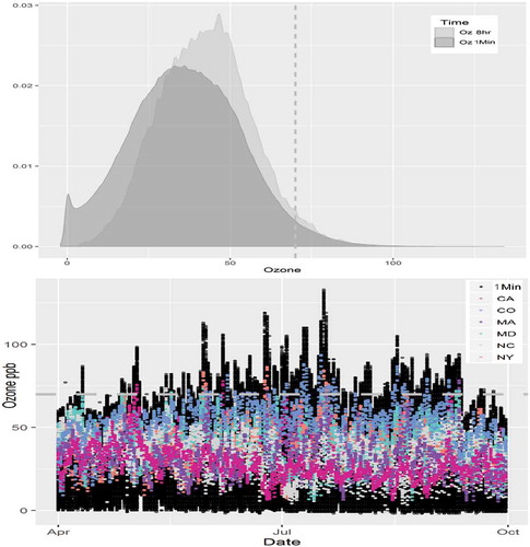
Figure 1 shows the density of 1-min ozone concentrations and corresponding maximum 8-hr block averages for Village Green bench and FEM monitoring station data. The vertical dashed line represents 70 ppb, which is the level of the 8-hr NAAQS and divides the AQI category of “Moderate” from the category “Unhealthy for Sensitive Groups.” It can be seen that the 1-min concentrations exhibited higher values (a longer upper tail) and the bulk of the distribution of the maximum 8-hr block averages is shifted slightly higher than the corresponding 1-min concentrations. This shift is likely due to the use of maximum 8-hr block averages. These showcase the similar distribution characteristics, but not a direct 1-to-1 relationship of 1-min concentrations to longer term averages. Note that the density plot considers relative frequency (y-axis). The time series of 1-min ozone concentrations across six FEM monitoring stations (CA, CO, MA, MD, NC, NY) and the corresponding maximum 8-hr block averages for the 2013 ozone season (April–September) are shown in the bottom plot of Figure 1. The 1-min concentrations exhibit higher individual values, and the seasonal peaks can be seen in the summer for both the 1-min and maximum 8-hr averages. Regional trends are also shown. The northern California sites (magenta) exhibit lower maximum 8-hr block averages than those in Colorado (light blue), and 8-hr averages in North Carolina (light gray) are always less than 70 ppb, with New York (orange) and Colorado exceeding 70 ppb multiple times throughout the 2013 ozone season.

Figure 1. Ozone density and time series. Top: Density of 1-minute ozone concentrations (dark grey) and corresponding maximum 8-hour block averages (light grey) for Village Green Bench and FEM monitoring station data. The dashed vertical line is 70 ppb. Bottom: 1-minute ozone concentrations (black) and corresponding maximum 8-hour block averages (colored by state) for the FEM sites in 6 states (CA, CO, MA, MD, NC, NY) for the 2013 ozone season (April–Sept). The dashed horizontal line represents 70 ppb.

PM_2.5

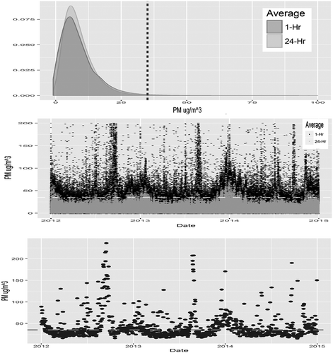
The distribution of the PM_2.5 1-hr averages versus 24-hr averages across all 386 monitoring stations is shown in Figure 2. Note that the full range of hourly PM_2.5 averages, –1 μg/m³ (EPA, 2015a) to 1167 μg/m³, with less than 1.4% of the 1-hr averages below 0 μg/m³ and approximately 1.4% greater than 35 μg/m³, are considered for the analysis along with the corresponding 24-hr averages (15 to 236 μg/m³). However, the distribution is truncated at 100 μg/m³ for display purposes. The vertical dashed line represents 35 μg/m³, which is the level is of the PM_2.5 24-hr NAAQS, and divides the AQI categories “Moderate” and “Unhealthy for Sensitive Groups.” It can be seen that the 1-hr averages exhibited higher values (a longer upper tail) and that the bulk of the distribution of the 1-hr averages is shifted higher than the 24-hr averages. These showcase the similar distribution characteristics but not direct a 1-to-1 relationship of short-term averages to longer term averages. The time series of PM_2.5 1-hr averages and corresponding 24-hr averages can be seen in the middle plot of Figure 2. The horizontal dashed line indicates 35 μg/m³. The 1-hr averages exhibit higher values, and the peaks of the 1-hr averages are mimicked on a reduced scale with the 24-hr averages. Approximately 1.3% of the 1-hr averages exceeded 35 μg/m³, observed across 375 sites and on all 1096 days. Approximately 0.6% of the 24-hr averages over 467 days exceeded 35 μg/m³ across 205 sites. The bottom plot of Figure 2 displays the time series of the U.S. daily maximum 24-hr average PM_2.5 across all 386 monitoring stations, showing the 467 days out of 1096 that exhibited an exceedance of 35 μg/m³.

Figure 2. PM_2.5 density and time series. Top: Distribution of the 1-hour averages versus 24-hour average PM2.5 across all 386 monitoring stations. The vertical dashed line represents 35 μg/m³. The horizontal axis is truncated at 100 μg/m³ for display purposes only. Middle: Time series of 1-hour PM_2.5 averages and corresponding 24-hour average for the 386 monitoring stations. The vertical axis is truncated at 200 μg/m³ for display purposes only. Bottom: Time series of the daily maximum 24-hour average PM_2.5 across all 386 sites. Four hundred and sixty-seven days exhibited an exceedance of 35 μg/m³. The dashed horizontal line represents 35 μg/m³.

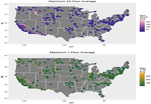
The spatial distribution of the maximum 1-hr average and the maximum 24-hr average, respectively, across all years at each site is exhibited in Figure 3. Note that while the scales are different, the trends are analogous. The higher averages (indicated by the lighter colors) are seen across both metrics in areas such as eastern California and Idaho/Montana/Wyoming.

Figure 3. PM_2.5 spatial trends. Spatial distribution of the PM_2.5 maximum 1-hour average (top) and the maximum 24-hour average (bottom) across all years at each site. Note the difference in scales across the two metrics.

Local pollutant patterns

While all available data were compiled to develop national breakpoints for ozone and PM_2.5 sensor message categories, analyses of individual locations show local and regional variation in air pollution levels. These analyses allow us to understand possible local events (e.g., near-source emission sources) and patterns in different areas of the country, which better informs low/medium/high breakpoints for each pollutant.

Ozone

The 1-min ozone measurements show regional differences across the 18 sites analyzed. The boxplots in Figure 4 show the distribution of 1-min ozone concentrations for Village Green bench and FEM monitoring station data for each of the 18 sites in the 9 states. The box represents the interquartile range: the bottom of the box is the first quartile (25th percentile), the middle line is the median or second quartile (50th percentile), and the top of the box is the third quartile (75th percentile). Table 1 shows the corresponding five-number summary (minimum, 1st quartile, median, 3rd quartile, maximum) for 1-min ozone concentrations at all 18 sites.

Table 1. Five-number summary (minimum, 1st quartile, median, 3rd quartile, maximum) for the 1-min ozone readings by site.

State	City	Minimum	1st Quartile	Median	3rd Quartile	Maximum
All	All	–2.0	24.2	36.0	48.0	134.0
CA-L	Livermore	–0.3	21.7	30.2	39.5	106.0
CA-S	Santa Rosa	–0.5	18.1	24.3	31.3	79.2
CO-D	Denver-Camp	0.0	27.0	39.0	49.0	109.0
CO-R	Rocky Flats	0.0	45.0	53.0	61.0	123.0
DC-D	DC	–2.0	16.6	30.7	43.8	118.3
KS-K	Kansas City	–2.0	15.7	27.9	37.6	115.7
MA-L	Lynn	0.0	29.0	37.0	46.0	120.0
MA-R	Roxbury	–2.0	19.0	28.0	36.0	112.0
MD-A	Aldino	0.0	31.0	41.0	51.0	133.0
MD-E	Essex	–1.0	28.0	40.0	50.0	134.0
MD-H	Howard University	–1.0	24.0	38.0	51.0	122.0
MD-R	Rockville	–1.0	25.0	38.0	51.0	106.0
NC-P	Pittsboro	–2.0	13.0	29.0	43.0	103.0
NC-R	Rockwell	–1.0	27.0	39.0	51.0	130.0
NC-D	Durham	–2.0	20.1	30.7	40.8	123.6
NY-C	CCNY	–2.0	20.0	30.0	42.0	131.0
NY-R	Riverhead	–2.0	31.0	39.0	49.0	134.0
PA-P	Philadelphia	–2.0	20.4	28.6	38.3	98.0

Figure 4. Regional ozone trends. Box plots of 1-minute ozone concentrations for Village Green bench and FEM monitoring station data across the 18 sites. The horizontal dashed line is at 70 ppb.

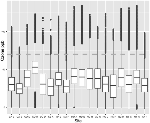
The vertical lines on each boxplot extend to 1.5 times the interquartile range (IQR: the first quartile subtracted from the third quartile) below and above the first and third quartiles, respectively, with concentrations beyond this represented by points. The horizontal dashed line across all boxplots represents 70 ppb. It can be seen that the distribution varies across states as well as within states. The distribution of ozone at the California sites near San Francisco (CA-L: Livermore, and CA-S: Santa Rosa) are lower overall than the sites in Colorado (CO-D: Denver Camp, and CO-R: Rocky Flats). The California sites have fewer concentrations above 70 ppb with the concentrations within 1.5 times the IQR all below 70 ppb, whereas the concentrations within 1.5 times the IQR at Colorado sites extend above 70 ppb. This is also the case for the concentrations at the DC, MD, NC, and NY sites. While several sites have third quartiles that are at or around 50 ppb, Rocky Flats, CO (CO-R) is the only site where the median (second quartile) exceeds 50 ppb. The variation is represented by the length of the box—a shorter box indicates a tighter distribution around the median with less spread; a longer box represents more variation in the concentrations. Santa Rosa, CA (CA-S), and Rocky Flats, CO (CO-R), have short boxes indicating lower variation, whereas Kansas (KS-S: Kansas City) and Pittsboro, NC (NC-P), have higher variation (longer boxes).

PM_2.5

Short-term (i.e., minutes to hours) concentrations of PM_2.5 can vary substantially, with the potential for higher concentrations near sources of PM emissions. For example, outdoor PM_2.5 concentrations ranging from less than 100 μg/m³ to more than 1000 μg/m³ have been reported in the vicinity of ongoing roadwork and on or near diesel buses (Hill et al., 2005). Indoor concentrations of PM can also be elevated near sources. For instance, indoor PM_2.5 concentrations have been shown to exceed 100 μg/m³ in designated smoking areas (Proescholdbell et al., 2009; King et al., 2012) and near other sources such as burning candles and cooking operations (Hammond et al., 2014). In some instances, indoor PM_2.5 concentrations were shown to exceed 1000 μg/m³ (Hammond et al., 2014). Therefore, PM_2.5 concentrations near sources were also taken into consideration for setting message category breakpoints. As discussed in “Interpretation and Communication of Short-term Air Sensor Data: A Pilot Project,” available at https://www.epa.gov/air-research/communicating-instantaneous-air-quality-data-pilot-project, sensor messages for the Low and Medium categories for PM_2.5 reflect the use of 1-hr average, rather than 1-min, PM_2.5 concentrations. Given the potential for near-source PM_2.5 concentrations to be much higher than those measured at existing ambient monitors, sensor messages for the “High” to “Very High” categories reflect the consideration of possible near-source concentrations based on averaging periods as short as 1-min. We address the use of 1-hr averages in our accompanying messages by making the link between 1-min concentrations and 1-hr averages an explicit focus the “Medium” category.

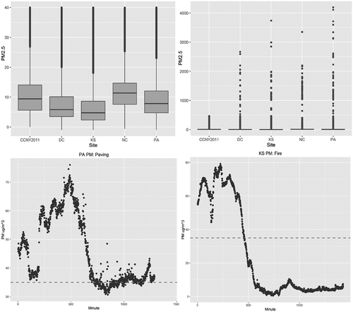
The 1-min PM_2.5 concentrations considered in the small-scale local case studies show regional differences and provide information about short-term events and trends. The full range of 1-min PM_2.5 concentrations (–1 to 4196 μg/m³) was considered. Approximately 1.0% of concentrations were less than 0 μg/m³. The 99th percentile was 38.8 μg/m³ with 85.4% of the concentrations at or below 35 μg/m³. The top plots in Figure 5 show the range of 1-min concentrations across the 5 sites with available 1-min PM_2.5 measurements. Note that the median in NC is the highest, 11.4 μg/m³, versus the next highest in NY at 8.0 μg/m³; however, the interquartile range is wider (5.7 to 14.2 in NY versus 7.6 to 14.7 in NC) in NY indicating more variation among the PM_2.5 measurements in NY. The bottom plots (Figure 5) showcase individual events of interest where high 1-min readings of PM_2.5 were observed in conjunction with paving in PA and wildfires in Canada reaching KS. Table 2 shows the five number summary for 1-min PM_2.5 readings across the 5 sites with available 1-min data.

Table 2. Five number summary (minimum, 1st quartile, median, 3rd quartile, maximum) for the 1-min PM_2.5 readings by site.

Site	Minimum	1st Quartile	Median	3rd Quartile	Maximum
All	–1.0	4.4	8.1	12.9	4196.0
CCNY	0.0	5.7	9.4	14.2	464.7
DC	–1.0	3.5	5.9	10.2	2671.0
KS	–1.0	2.3	4.8	8.8	3740.0
NC	–0.6	7.6	11.4	14.7	3351.0
PA	–1.0	4.8	8.0	12.4	4196.0

Figure 5. Regional PM_2.5 trends. Top: Distribution of 1-minute PM_2.5 measurements across the 5 sites. The left plot is truncated at 40 μg/m³ to show the characteristics of the bulk of the distribution, while the right plot shows the full range of concentrations measured. Bottom: PM_2.5 Events: 1-Minute Village Green Data trends on September 2, 2015 in Philadelphia during street paving (left plot) and on July 7, 2015 in Kansas City due to a smoke plume from a Canadian wildfire (right plot).

Methodology

This section explains the methodology for considering the empirical distributions of the 8-hr averages (ozone) and 24-hr averages (PM_2.5), given the corresponding short-term concentrations from sensors. This enables a probabilistic assessment of the corresponding longer-term averages that are likely to be associated with given short-term measurements.

For ozone, we consider how the 1-min concentrations and the distribution of their corresponding maximum 8-hr block averages relate to the ozone NAAQS and to breakpoints for the AQI categories for “Good,” “Moderate,” “Unhealthy for Sensitive Groups,” and “Unhealthy.” Sensor messages for the public will be grouped into corresponding “Low,” “Medium,” “High,” and “Very High” categories. A “Very High” reading, while expected to be a rare occurrence, could indicate an unusually high concentration or a malfunctioning sensor. Similarly, for PM_2.5, we investigated the relationships between 1-hr and 24-hr average PM_2.5 concentrations to inform the identification of PM_2.5 sensor breakpoints and messages. For the “High” category, we also considered near-source concentrations. A “Very High” PM_2.5 concentration is expected to be a rare occurrence, but could occur during extreme situations such as wildfires, or near some common PM sources (e.g., diesel buses, designated smoking areas, candles, cooking). For each pollutant, a range of possible breakpoints was explored and the corresponding breakpoint probabilities were considered.

Breakpoint probabilities for the different message categories represent the empirical probability of the maximum 8-hr block average (ozone) or the 24-hr average (PM_2.5) exceeding specific AQI breakpoints, given that the observed 1-min concentration (ozone) or 1-hr average (PM_2.5) falls within a specified range. The specified ranges correspond to considerations for the possible “Low,” “Medium,” and “High” message categories. The corresponding distribution is examined to determine the probability that the maximum 8-hr block average for ozone (or 24-hr average for PM_2.5) exceeds the various AQI breakpoint ranges. These are conditional probabilities, conditioned on the observance of a given 1-min concentration within a specified Low/Medium/High messaging category. No distributional or modeling assumptions are made about the underlying characteristics of the data and their corresponding behavior and/or distributional properties. This allows for a robust, empirical comparison of events that occur relatively infrequently, which is the area of interest for air quality exceedances and public health concerns. The development of messages corresponding to the selected breakpoints, and the policy considerations for such, are outlined in “Interpretation and Communication of Short-term Air Sensor Data: A Pilot Project,” available at https://www.epa.gov/air-research/communicating-instantaneous-air-quality-data-pilot-project.

The empirical frequencies (%) for the message categories “Low,” “Medium,” and “High” were also considered. Messaging frequencies are not conditional probabilities—they simply represent the frequency with which the range of concentrations corresponding to a given message (e.g., “High”) is observed at the corresponding breakpoint. Note that these frequencies are based on short-term readings, which are correlated (i.e., high concentrations of ozone and PM_2.5 likely occur near other high concentrations).

The scales and messages described in this paper are based on analyses of U.S. air quality data; as such, they are appropriate only for use in the United States. This analysis is focused strictly on relating short-term concentrations to longer averages. It does not address interpreting sensor data (with all of its uncertainties and precision issues) relative to Federal Reference Monitor (FRM)/FEM monitors that report the AQI or how different types of sensors relate to FRM/FEM data. Additionally, this analysis focused only on the outdoor environments and stationary monitors. Different environments (e.g., indoor) and different sensor modes (e.g., fixed versus portable, mobile, personal) could introduce additional uncertainties and may require additional considerations. This information is intended to provide users an additional tool for understanding air quality and exposures, and for planning outdoor activities.

Results

Ozone

We considered the empirical distribution of the maximum 8-hr block averages, given the corresponding 1-min concentrations used in the calculation of the maximum 8-hr block averages. The 8-hr block averages are considered for 1-min concentrations that fall within a specified range under consideration for messaging breakpoints. “Low” to “Medium” category breakpoints of 55, 60, 65, and 70 ppb were considered along with “Medium” to “High” category breakpoints of 85, 90, 95, and 100 ppb. Thus, 16 sets of possible breakpoint messaging ranges were explored. The example detailed in Figure 6 and Tables 3 and 4 is for the possible “Low” range of 0–59 ppb with corresponding “Medium” range of 60–89 ppb. The general trend shown in Figure 6 is that lower 8-hr block averages are associated with lower 1-min concentrations. For example, it is shown in the top plot in Figure 6 that for 1-min concentrations in the range 0–59 ppb, only 12% of the corresponding 8-hr block averages are above 55 ppb and only 1% are above 70 ppb. Similarly, the trend among the higher values is that higher 8-hr block averages are associated with higher 1-min concentrations. A set of histograms and tables considering the full implementation of possible “Low,” “Medium,” and “High” ozone (and PM_2.5) breakpoints can be found at https://www.epa.gov/air-research/communicating-instantaneous-air-quality-data-pilot-project.

Table 3. Breakpoints for ozone message categories.

Preliminary sensor breakpoints for ozone,* not for regulatory purposes		Empirical messaging frequencies (%)
Low	0–59 ppb	91.1
Medium	60–89 ppb	8.6
High	90–149 ppb	0.3
Very High**	>150 ppb	0.0

*May be refined as data sources are periodically updated.

**In this study there were no ozone readings above 150 ppb.

Table 4. Percent of maximum 8-hr block average for corresponding 1-min ozone in AQI categories for selected message categories.

AQI breakpoints (category)	Low: 0–59	Medium: 60–89	High: 90–149
Percent 8 hr >55 (Above Good)	12	92	100
Percent 8 hr 55 to 70 (Moderate)	11	64	5
Percent 8 hr >70 (Above Moderate)	1	28	95
Percent 8 hr 70 to 85 (Unhealthy for Sensitive Groups)	1	26	46
Percent 8 hr >85 (Unhealthy)	0	2	49

Figure 6. Ozone conditional distribution. Conditional distribution of maximum 8-hour block averages for the possible sensor messaging categories and the corresponding AQI breakpoints. Zero to 59 ppb is the range considered for the “Low” category, 60–89 ppb are considered for “Medium,” and greater than or equal to 90 ppb considered for “High.” The vertical dashed line indicates 70 ppb. Note. While the analysis includes the full range of data, for display purposes only the x-axis is truncated to 100 ppb.

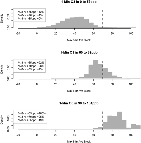
The empirical messaging frequencies for ozone are also shown in Table 3. Table 3 shows that 1-min concentrations in the range 0–59 ppb occurred with a relative frequency of 91.1%. Therefore, a “Low” message was observed approximately 91.1% of the time for a “Low” range of 0–59 ppb. Given a “Medium” range of 60–89 ppb, the “Medium” message was seen with a relative frequency of 8.6%. Table 3 indicates that “High” occurred with a relative frequency of 0.3%. The empirical frequency for ozone concentrations >150 ppb was 0%.

A “Low” sensor reading generally occurs when the corresponding 8-hr average concentration is likely to be below the level of the NAAQS and is in the “Good” or “Moderate” AQI categories. A “Medium” sensor reading generally occurs when the corresponding 8-hr average concentration is likely to be in the “Moderate” or “Unhealthy for Sensitive Groups” AQI categories. A “High” sensor reading generally occurs when the corresponding 8-hr average concentration is likely to be above the level of the NAAQS and in the “Unhealthy for Sensitive Groups” or above AQI categories. Table 4 displays the distribution of the maximum 8-hr block average for 1-min ozone concentrations across the different “Low,” “Medium,” and “High” message categories and corresponding AQI categories. For example, if Low was set at 0–59 ppb for 1-min concentrations, the maximum 8-hr block average was above 55 ppb in the “Moderate” and above AQI categories with 12% relative frequency, with 1% “Unhealthy for Sensitive Groups” and 0% frequency in “Unhealthy” (>85 ppb). For the “Medium” category set at 60 ppb–89 ppb, 92% were above the “Good” category, with 64% in the “Moderate” AQI category, 26% in “Unhealthy for Sensitive Groups,” and 2% “Unhealthy.” For the “High” category set at 90–150 ppb, approximately 100% of the corresponding maximum 8-hr block averages were above the “Good” AQI category (≥55 ppb) and 95% above “Moderate” (≥70 ppb), with 43% in “Unhealthy for Sensitive Groups” and 49% in “Unhealthy.” A full set of tables considering the full range of possible “Low,” “Medium,” and “High” ozone breakpoints can be found at https://www.epa.gov/air-research/communicating-instantaneous-air-quality-data-pilot-project.

PM_2.5

We considered the empirical distribution of the 24-hr averages given the corresponding 1-hr averages used in the calculation of the 24-hr averages. The 24-hr averages are considered for 1-hr averages that fall within a specified range under consideration for message category breakpoints. Lower breakpoints of 12, 15, 20, 25, 30, 35, 40, and 45 μg/m³ were considered for the break between the “Low” and “Medium” categories, along with “Medium” category upper breakpoints of 50, 55, 60, and 65 μg/m³. Thus 36 total sets of possible breakpoint messaging ranges were explored. For the “Low” range of 0–29 μg/m³, Figure 7 shows the distribution of 24-hr averages for the 1-hr average in the range of 0–29 μg/m³ for the “Low” category, 30–69 μg/m³ as the consideration for the “Medium” category, and ≥70 μg/m³ for “High.” Additional consideration was given to the upper range 70, 75, 70, and 85 μg/m³ for a “Low/Medium” breakpoint of 30 μg/m³ (not shown). The general trend shows that lower 24-hr averages are associated with lower 1-hr averages. For example, it is shown in the middle plot in Figure 7 that for 1-hr averages in the range 30-69 μg/m³, only 19% of the corresponding 24-hr averages are above 35 μg/m³, and only 3% are above 55 μg/m³. Similarly, the trend among the higher values is that higher 24-hr averages are associated with higher 1-hr averages.

Figure 7. PM_2.5 conditional distribution. Conditional distribution of 24-hour averages for the possible sensor messaging categories and the corresponding AQI breakpoint ranges for the “Medium” category considerations with a low breakpoint of 29 μg/m³. The vertical blue line represents 35 μg/m³. Note. While the analysis includes the full range of data, for display purposes only the x-axis is truncated to 100 μg/m³.

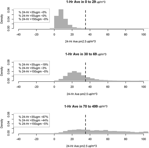
The empirical messaging frequencies for PM_2.5 are also shown in Table 5. For example, 1-hr averages in the range 0–29 μg/m³ were observed with a relative frequency of 97.9%. Therefore, a “Low” message would be observed approximately 97.9% of the time for a “Low” range of 0–29 μg/m³. Given a “Medium” range of 30–69 μg/m³, the “Medium” message would be seen with a relative frequency of 1.9%. Table 5 indicates that “High” would be observed with a relative frequency of 0.2%.

Table 5. Breakpoints for PM_2.5 message categories.

Preliminary sensor messages for PM2.5,* not for regulatory purposes		Empirical messaging frequencies (%)
Low	0–29 µg/m^3	97.9
Medium	30–69 µg/m^3	1.9
High	70–499 µg/m^3	0.2
Very High	>500 µg/m^3	~0.0**

*May be refined as data sources are periodically updated.

**Out of approximately 7 million readings only 35 exceeded 500 µg/m³.

A “Low” sensor reading outdoors almost always occurs when the corresponding 24-hr average PM_2.5 concentration is below the level of the 24-hr NAAQS and is in the “Good” or “Moderate” AQI categories. A “Medium” sensor reading generally occurs when the corresponding PM_2.5 concentration is in the “Moderate” or “Unhealthy for Sensitive Groups” AQI categories. A “High” sensor reading corresponds to concentrations that can occur near sources. Table 6 displays the distribution of 24-hr averages for the 1-hr PM_2.5 averages across the different “Low,” “Medium,” and “High” messaging categories and corresponding AQI categories. Table 6 shows that if “Low” was set at 0–29 µg/m³, 0% of the time the 24-hr average would be above 35 µg/m³ into the “Unhealthy for Sensitive Groups” and above AQI categories. For “Medium” set to 30–69 μg/m³, 19% would be above “Moderate,” with 16% in the “Unhealthy for Sensitive Groups” AQI category, and 3% in “Unhealthy,” with approximately zero observed probability of exceeding 150 µg/m³ (Very Unhealthy–Hazardous). For “High” set to 70–499 μg/m³, 67% would be above “Moderate” and 23% would be in the “Unhealthy for Sensitive Groups” category. Forty-four percent of the time the 24-hr average would fall in the range 55–150 μg/m³ in the “Unhealthy” AQI category and 5% exceeding 150 µg/m³ in the “Very Unhealthy–Hazardous” AQI category. A full set of tables considering the full range of possible “Low,” “Medium,” and “High” ozone breakpoints can be found at https://www.epa.gov/air-research/communicating-instantaneous-air-quality-data-pilot-project.

Table 6. Percent of 24-hr averages for corresponding 1-hr average PM_2.5 in AQI categories for selected message categories.

AQI breakpoints (category)	Low: 0–29	Medium: 30–69	High: 70–499
Percent average >35 (Above Moderate)	0	19	67
Percent average 35 to 55 (Unhealthy for Sensitive Groups)	0	16	23
Percent average >55 (Above Unhealthy for Sensitive Groups)	0	3	44
Percent average 55 to 150 (Unhealthy)	0	3	39
Percent average >150 µg/m^3 (Very Unhealthy–Hazardous)	0	0	5

Discussion

Real-time sensors have the potential to provide important information about fine-scale current air quality and local air quality events. The analysis of short-term readings showed interesting characteristics of ozone and PM_2.5 that are not immediately evident when considering only longer term averages. This can be seen in the case studies in which the short-term readings captured the paving and wildfire source events. We are also able to see similar patterns in the spatial and temporal characteristics of the short-term measurements that are mimicked in the longer term average trends though on a different scale (Figures 2 and 3), with the short-term measurements offering current information about the local air quality.

The increased availability of real-time data from air sensors creates a need for the interpreting of such information. The analysis of short-term data and comparison to longer term averages can be used to support communication strategies for air sensor data so that EPA, states, sensor manufacturers, and users interpret short-term data in a consistent manner. To inform suggested breakpoints and messages, important considerations include relating the information to available health messaging that can be supported by scientific studies of health effects, as well as the quality of sensor data. It is again important to note that sensor technologies are often not operated in accordance with federal quality assurance and operating procedures—introducing important considerations about uncertainty and interpretation when evaluating sensor measurements. In this analysis, the quality of the data from the Village Green sites and FEM monitors is well characterized; however, the relationships observed between 1-min readings and longer term averages may not hold for readings from other portable sensors.

The analysis presented here provides an empirical technique for assessment and context for the interpretation of sensor data as they relates to the NAAQS and the AQI, which is used throughout the United States to communicate daily air quality to the public. This analysis provides insight into the relationship between short-term sensor readings and longer term averages of pollutant concentrations. The statistical analysis of short-term regulatory and sensor data, coupled with policy considerations and known health effects experienced over longer averaging times, supports interpretation of such short-term data and efforts to communicate local air quality. Future work includes study of additional pollutants, as well as incorporating additional short-term data as they become available. Additional analysis will also be needed to compare sensor concentrations to FRM/FEM data for accuracy and precision. Further study is also needed to understand the relationship between short-term concentrations and longer term averages in different types of environments (e.g., indoor, outdoor, near sources), as well as for different sensor modes (fixed, portable, mobile, and personal).

Acknowledgment

The authors thank the entire EPA Air Sensors Team, including but not limited to those who specifically provided input on the data, analysis, and/or methods: Ron Evans, Brett Gantt, Gayle Hagler, Bryan Hubbell, Jesse McGrath, Liz Naess, Ben Wells, Karen Wesson, and Ronald Williams.

Additional information

Notes on contributors

Elizabeth Mannshardt

The authors are colleagues in EPA’s Office of Air Quality Planning and Standards in Research Triangle Park, North Carolina. Elizabeth Mannshardt is a Statistician; Kristen Benedict is a Physical Scientist; David Mintz is a Senior Statistician; and Richard Wayland is the Division Director in the Air Quality Assessment Division. Martha Keating is a Policy Advisor; Scott Jenkins is a Senior Environmental Health Scientist; and Susan Stone is a Senior Environmental Health Scientist, all with the Health and Environmental Impacts Division.

Kristen Benedict

The authors are colleagues in EPA’s Office of Air Quality Planning and Standards in Research Triangle Park, North Carolina. Elizabeth Mannshardt is a Statistician; Kristen Benedict is a Physical Scientist; David Mintz is a Senior Statistician; and Richard Wayland is the Division Director in the Air Quality Assessment Division. Martha Keating is a Policy Advisor; Scott Jenkins is a Senior Environmental Health Scientist; and Susan Stone is a Senior Environmental Health Scientist, all with the Health and Environmental Impacts Division.

Scott Jenkins

The authors are colleagues in EPA’s Office of Air Quality Planning and Standards in Research Triangle Park, North Carolina. Elizabeth Mannshardt is a Statistician; Kristen Benedict is a Physical Scientist; David Mintz is a Senior Statistician; and Richard Wayland is the Division Director in the Air Quality Assessment Division. Martha Keating is a Policy Advisor; Scott Jenkins is a Senior Environmental Health Scientist; and Susan Stone is a Senior Environmental Health Scientist, all with the Health and Environmental Impacts Division.

Martha Keating

The authors are colleagues in EPA’s Office of Air Quality Planning and Standards in Research Triangle Park, North Carolina. Elizabeth Mannshardt is a Statistician; Kristen Benedict is a Physical Scientist; David Mintz is a Senior Statistician; and Richard Wayland is the Division Director in the Air Quality Assessment Division. Martha Keating is a Policy Advisor; Scott Jenkins is a Senior Environmental Health Scientist; and Susan Stone is a Senior Environmental Health Scientist, all with the Health and Environmental Impacts Division.

David Mintz

The authors are colleagues in EPA’s Office of Air Quality Planning and Standards in Research Triangle Park, North Carolina. Elizabeth Mannshardt is a Statistician; Kristen Benedict is a Physical Scientist; David Mintz is a Senior Statistician; and Richard Wayland is the Division Director in the Air Quality Assessment Division. Martha Keating is a Policy Advisor; Scott Jenkins is a Senior Environmental Health Scientist; and Susan Stone is a Senior Environmental Health Scientist, all with the Health and Environmental Impacts Division.

Susan Stone

The authors are colleagues in EPA’s Office of Air Quality Planning and Standards in Research Triangle Park, North Carolina. Elizabeth Mannshardt is a Statistician; Kristen Benedict is a Physical Scientist; David Mintz is a Senior Statistician; and Richard Wayland is the Division Director in the Air Quality Assessment Division. Martha Keating is a Policy Advisor; Scott Jenkins is a Senior Environmental Health Scientist; and Susan Stone is a Senior Environmental Health Scientist, all with the Health and Environmental Impacts Division.

Richard Wayland

The authors are colleagues in EPA’s Office of Air Quality Planning and Standards in Research Triangle Park, North Carolina. Elizabeth Mannshardt is a Statistician; Kristen Benedict is a Physical Scientist; David Mintz is a Senior Statistician; and Richard Wayland is the Division Director in the Air Quality Assessment Division. Martha Keating is a Policy Advisor; Scott Jenkins is a Senior Environmental Health Scientist; and Susan Stone is a Senior Environmental Health Scientist, all with the Health and Environmental Impacts Division.

References

- 64 FR 42530. 1999. National Ambient Air Quality Standards for Ozone (Air Quality Index Reporting). August 4. https://www2.ed.gov/legislation/FedRegister/finrule/1999-1/031299e.pdf (accessed January 5, 2017).
- Bell, M.L., K. Ebisu, R.D. Peng, J. Walker, J.M. Samet, S.L. Zeger, and F. Dominici. 2008. Seasonal and regional short-term effects of fine particles on hospital admissions in 202 U.S. counties, 1999–2005. Am. J. Epidemiol. 168:1301–1310. doi:10.1093/aje/kwn252.
- Centers for Disease Control and Prevention. 2012. Indoor air quality at nine large-hub airports with and without designated smoking areas—United States, October–November 2012. Morbid. Mortal. Weekly Rep. 61(46):948–51. http://www.cdc.gov/mmwr/preview/mmwrhtml/mm6147md.htm
- Chang, H.H, B.J. Reich, and M.L. Miranda. 2012. Time-to-event analysis of fine particle air pollution and preterm birth: Results from North Carolina, 2001–2005. Am. J. Epidemiol. 175:91–98. doi:10.1093/aje/kwr403
- Hammond, D., C. Crogham, H. Shin, R. Burnett, R. Bard, R.D. Brooks, and R. Williams. 2014. Cardiovascular impacts and micro-environmental exposure factors associated with continuous peronsal PM2.5 monitoring. J. Expos. Sci. Environ. Epidemiol. 24:337–45. doi:10.1035/jes.2013.46
- Hill L.B., N.J. Zimmerman, and J.A. Gooch. 2005. A multi-city investigation of the effectiveness of retrofit emissions controls in reducing exposures to particulate matter in school buses. Clean Air Task Force. http://www.catf.us/resources/publications/view/82 (accessed January 5, 2017).
- Jerrett, M., R.T. Burnett, C.A. Pope III, K. Ito, G. Thurston, D. Krewski, Y. Shi, E. Calle, and M. Thun. 2009. Long-term ozone exposure and mortality. N. Engl. J. Med. 360:1085–95. doi:10.1056/NEJMoa0803894
- Jiao, W.G., S.W. Hagler, R.W. Williams, R.N. Sharpe, L. Weinstock, and J. Rice. 2015. Field assessment of the Village Green Project: An autonomous community air quality monitoring system. Environ. Sci. Technol. 49(10): 6085–92. doi:10.1021/acs.est.5b01245
- Katsouyanni, K., J.M. Samet, H.R. Anderson, R. Atkinson, A. Le Tertre, S. Medina, E. Samoli, G. Touloumi, R.T. Burnett, D. Krewski, T. Ramsay, F. Dominici, R.D. Peng, J. Schwartz, and A. Zanobetti. 2009. Air pollution and health: A European and North American approach (APHENA). Research report 142. Boston, MA: Health Effects Institute. http://pubs.healtheffects.org/view.php?id=327.
- Krewski, D., M. Jerrett, R.T. Burnett, R. Ma, E. Hughes, Y. Shi, M.C. Turner, A.C. Pope III, G. Thurston, E.E. Calle, and M.J. Thun. 2009. Extended follow-up and spatial analysis of the American Cancer Society study linking particulate air pollution and mortality. HEI Research Report 140. Health Effects Institute, Boston, MA. http://pubs.healtheffects.org/view.php?id=315.
- Laden, F., J. Schwartz, D. Speizer, and D.W. Dockery. 2006. Reduction in fine particulate air pollution and mortality: extended follow-up of the Harvard Six Cities Study. Am. J. Respir. Crit. Care Med. 173:667–72. doi:10.1164/rccm.200503-443OC
- Pope C.A., D.W. Dockery, and J. Schwartz. 1995. Review of epidemiological evidence of health effects of particulate air pollution. Inhal. Toxicol. 7:1–18. doi:10.3109/08958379509014267
- Pope, C.A. III, and D.W. Dockery. 2006. Health effects of fine particulate air pollution: Lines that connect. J. Air Waste Manage. Assoc. 561:709–742. doi:10.1080/10473289.2006.10464485
- Proescholdbell S., J. Steiner, A. O. Goldstein, and S.H. Malek. 2009. Using indoor air quality monitoring in 6 counties to change policy in North Carolina. Prevent. Chronic Dis. 6(3): A88. http://www.cdc.gov/pcd/issues/2009/jul/08_0115.htm.
- Reich, B.J., M. Fuentes, and J. Burke. 2009. Analysis of the effects of ultrafine particulate matter while accounting for human exposure. Environmetrics 20:131–46. doi:10.1002/env.v20:2
- U.S. Code. 1990. Title 42: The Public Health and Welfare, Chapter 85. http://uscode.house.gov/view.xhtml?path=/prelim@title42/chapter85&edition=prelim (accessed January 5, 2017).
- U.S. Environmental Protection Agency. 2009. Final Report: Integrated Science Assessment for Particulate Matter, Chap. 2.3. Washington, DC: U.S. Environmental Protection Agency. EPA/600/R-08/139F.
- U.S. Environmental Protection Agency. 2013. Final Report: Integrated Science Assessment of Ozone and Related Photochemical Oxidants, Chap. 2.5. Washington, DC: U.S. Environmental Protection Agency. EPA/600/R-10/076F, 2013.
- U.S. Environmental Protection Agency. 2015a. Quality Assurance Project Plan, Village Green Project—Self powered, real-time air monitoring. Category IV/measurement project. https://www.epa.gov/air-research/village-green-project (accessed January 5, 2017).
- U.S. Environmental Protection Agency. 2015b. Village Green. http://villagegreen.airnowtech.org/welcome (accessed February 6, 2017).
- World Health Organization. 2000. Evaluation and use of epidemiological evidence for environmental health risk assessment. Regional Office for Europe, Guideline document, EUR/00/5020369. http://www.euro.who.int/__data/assets/pdf_file/0006/74733/E68940.pdf (accessed January 5, 2017).
- Zanobetti, A., and J. Schwartz. 2009. The effect of fine and coarse particulate air pollution on mortality: A national analysis. Environ. Health Perspect. 117:1–40. doi:10.1289/ehp.0800108