Evaluation of air quality zone classification methods based on ambient air concentration exposure

ABSTRACT

Air quality zones are used by regulatory authorities to implement ambient air standards in order to protect human health. Air quality measurements at discrete air monitoring stations are critical tools to determine whether an air quality zone complies with local air quality standards or is noncompliant. This study presents a novel approach for evaluation of air quality zone classification methods by breaking the concentration distribution of a pollutant measured at an air monitoring station into compliance and exceedance probability density functions (PDFs) and then using Monte Carlo analysis with the Central Limit Theorem to estimate long-term exposure. The purpose of this paper is to compare the risk associated with selecting one ambient air classification approach over another by testing the possible exposure an individual living within a zone may face. The chronic daily intake (CDI) is utilized to compare different pollutant exposures over the classification duration of 3 years between two classification methods. Historical data collected from air monitoring stations in Kuwait are used to build representative models of 1-hr NO₂ and 8-hr O₃ within a zone that meets the compliance requirements of each method. The first method, the “3 Strike” method, is a conservative approach based on a winner-take-all approach common with most compliance classification methods, while the second, the 99% Rule method, allows for more robust analyses and incorporates long-term trends. A Monte Carlo analysis is used to model the CDI for each pollutant and each method with the zone at a single station and with multiple stations. The model assumes that the zone is already in compliance with air quality standards over the 3 years under the different classification methodologies. The model shows that while the CDI of the two methods differs by 2.7% over the exposure period for the single station case, the large number of samples taken over the duration period impacts the sensitivity of the statistical tests, causing the null hypothesis to fail. Local air quality managers can use either methodology to classify the compliance of an air zone, but must accept that the 99% Rule method may cause exposures that are statistically more significant than the 3 Strike method.

Implications: A novel method using the Central Limit Theorem and Monte Carlo analysis is used to directly compare different air standard compliance classification methods by estimating the chronic daily intake of pollutants. This method allows air quality managers to rapidly see how individual classification methods may impact individual population groups, as well as to evaluate different pollutants based on dosage and exposure when complete health impacts are not known.

Introduction

Ambient air quality standards are specified by most countries to protect human health and reduce impacts of hazardous air pollution emissions for the public welfare. The Clean Air Act of 1970 (1970 CAA) was one of the first national legislations that established national-wide concentration levels for ambient air quality. The original 1970 CAA National Ambient Air Quality Standards (NAAQS) included six criteria air pollutants (CAPs) with both primary (human health) and secondary (public welfare such as visibility, crops, and building material) standards (EPA, 1970). A standard is assumed to be a specific air pollutant, with its threshold concentration value and the averaging time associated with the concentration value. In some cases, pollutants have multiple standards, such as nitrogen dioxide (NO₂), which has a 1-hr average standard (100 ppb, 98th percentile of 1-hr daily maximum concentrations, averaged over 3 years) and an annual average standard (53 ppb, annual mean). The current NAAQS includes 7 air pollutant categories and 12 different standards. European air standards began with levels for sulfur dioxide and suspended particulates in 1980 (European Economic Community [EEC], 1980). The World Health Organization (WHO) published recommended air quality guidelines (AGQs) as early as 1987 for Europe, with ambient levels and averaging periods for 28 different chemicals and 39 standards (Lubkert-Alcamo, 1994). The current European air quality directive was adopted in 2008 and includes 12 different air pollutants with 15 different standards (European Union [EU], 2008), while a WHO AGQ update was published in 2005 with only five pollutants, but 25 standards (WHO, 2006).

Compliance classification

The averaging periods of each pollutant are not always clear in regard to when the measurement period begins and ends. By convention, most air monitoring stations (AMSs) follow the U.S. EPA required hourly average reporting that starts at the beginning of the hour and ends on the 59th minute (EPA, 2007). A similar convention holds for 24-hr averages whereby averaging starts at midnight (00:00 hrs) to 23:59 hr. Annual averages are based on calendar years, beginning on January 1 at 00:00 hr and ending on December 31 at 23:59 hr. In the case of particulate matter, reporting follows set 24-hr periods. The U.S. EPA method for taking 3-year averages is to average readings taken over individual quarters, average quarterly, and then average the quarters over 3 years (Cohen et al., 1999). International standards do not have this same level of detailed description for averaging, and it is the authors’ experience that U.S. EPA methodology is assumed when guidance or interpretation is not available.

What is less clear is how results from multiple monitoring stations in one air quality zone should be aggregated. In the United States, air quality zones are based on designated air quality control regions (AQCRs) that include municipalities and groups of intrastate and interstate counties (EPA, 1991). Currently there are 264 designated AQCRs with 121 in some form of noncompliance (or nonattainment) with the NAAQS (EPA, 2016b).

To determine whether an air quality zone is in or out of compliance with the local standards, AMSs are used to measure ambient air and weather conditions. The U.S. EPA uses a “winner-take-all” approach for some pollutants such as O₃ and PM_2.5 in that if one of the state and local air monitoring stations (SLAMS) within an AQCR registers exceedances that surpass a NAAQS standard, the entire zone is noncompliant (EPA, 2005a). Recently the U.S. EPA has considered a more tailored approach to O₃ nonattainment designations by allowing regional offices to work with states and Native American tribes to determine nonattainment areas based on local conditions and in some cases declare only part of an AQCR a nonattainment area (McCabe, 2015). We assume for the time being that the current “winner-takes-all” approach is still in effect and used by air managers in order to demonstrate our procedure.

In the California South Coast air basin, there are at least 43 active monitoring stations (California Air Resources Board [CARB], 2013) to cover 10,743 square miles (27,824 sq km) and protect approximately 17 million people (South Coast Air Quality Management District [AQMD], 2010). If only one station measures an exceedance of carbon monoxide (CO) over the standard, the entire basin is noncompliant and not just the immediate area. An air monitor is assumed to uniformly represent the air quality of the area around it. Murray and Newman (2014) recommend that lowest reading in a network area be used for multiple stations. This area could be as small as several hundred square meters in a microscale range of up to 100-m radius from the station, to a middle range (up to 0.5-km radius), neighborhood range (4-km radius), urban range (50-km radius) or regional range (several-hundred-kilometer radius) (Pan and Lee, 2009). Siting air monitoring stations is therefore a very important process that incorporates many variables to best represent the local area (Bermudez and Fine, 2010), but may not represent an entire region.

In 2012, the State of Kuwait issued the Kuwait Ambient Air Quality Standards (KAAQS) in order to update its air management program as part of the Kuwait Integrated Environmental Management System (KIEMS) sponsored by the United Nations Development Program (UNDP) with the Kuwait Environment Public Authority (KEPA). The new standards included a “winner-take-all” approach where an air zone was out of compliance for an air pollutant if any one AMS observed more than three observations (“3 strikes”) above the relevant standard’s threshold, or Guideline Value (GV), in a calendar year (KEPA, 2012). The KAAQS are shown in Table 1. The GVs are managed based on hourly measurements from AMSs with different averaging periods, but no daily maximums.

Table 1. Kuwait ambient air quality standards.

Pollutant	Guideline value	Averaging time
Carbon monoxide (CO)	30 mg/m^3 (26 ppm)	1 hr
	10 mg/m^3 (9 ppm)	8 hr
Nitrogen dioxide (NO2)	200 μg/m^3 (106 ppb)	1 hr
	40 μg/m^3 (21 ppb)	Annual
Sulfur dioxide (SO2)	20 μg/m^3 (8 ppb)	24 hr
	75 μg/m^3 (29 ppb)	1 hr
Ozone (O3)	100 μg/m^3 (51 ppb)	8 hr
Lead (Pb)	0.5 μg/m^3	Annual
Particulate material <10 µm (PM10)	90 μg/m^3	Annual
	150 μg/m^3	24 hr
Particulate material <2.5 µm (PM2.5)	15 μg/m^3	Annual
	35 μg/m^3	24 hr

Note. Conversion based on 1 ATM and 25 degrees Celsius.

The 3-Strike method was immediately considered too conservative and ambitious for a country with a relatively new air management program and a young environmental regulatory agency. While the intent of the program was to protect human health and welfare through robust air quality standards that industry and stakeholders would strive to meet, it was also considered too stringent in that it did not take into account annual impacts of industrial output and complex land–sea breeze (LSB) weather patterns. Another compliance classification method was considered whereby 3 years of air monitoring data was collected to account for industrial output variations and seasonal weather effects. With this method, if 99% of all hourly observations over the 3 years were less than or equal to the GV, then the zone was in compliance. If a zone had two or more AMSs, the measurements from individual stations would be pooled and the composite measurements evaluated to determine if they were ≤GV. This method was called the “99% Rule.” Using a percentile approach is similar to existing methods used by the U.S. EPA for 1-hr SO₂ and 1-hr NO₂, except the 99th percentile is used instead of the 98th (EPA, 2016a).

One of the drawbacks of the 99% Rule method was that if one station consistently measured high readings, it could drive the entire zone into a noncompliant status just like the 3-Strike method. This was considered an acceptable risk as the method incorporated 3 years of data instead of 1 year worth. A more significant issue, however, was, what exposure risk would the population living in a zone face if the zone were considered in compliance under a 3-Strike classification versus a 99% Rule classification? The research presented in the rest of this paper seeks to answer that question.

Materials and methods

Area of study

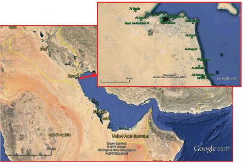
Kuwait is a small country of 17,818 km² located on the northwest corner of the Persian Gulf, at longitudes 46.56–48.37° east and latitudes 28.51–30.16° north with more than 499 km of coastline (CIA, 2015). It is bordered by Iraq to the north and Saudi Arabia to the south and west. The country is classified as a desert zone with the highest altitude reaching only 300 m above sea level. In 2011, approximately 3.1 million people lived in Kuwait (Central Statistical Bureau, Kuwait [CSB], 2014), with more than 64% of its annual gross domestic product (GDP) coming from the production of hydrocarbons (KAMCO, 2013). Other industries in Kuwait include power generation and water desalination using heavy oil and natural gas at five sites, steel making using electrical induction furnaces, and food preparation. The country has more than 7,400 km of paved roads and more than 1.8 million cars in service (CSB, 2014). More than 98% of the population live within 10 km of the coast and are subject to coastal effect winds, caused by the diurnal differential heating/cooling of the sea and land (Crosman and Horel, 2010; Cuxart et al., 2014). The land–sea breezes (LSB) shift direction and speed over the course of the day, recirculating pollution back and forth from land sources.

The Kuwait Environment Public Authority (KEPA) is responsible for monitoring environmental conditions and enforcing compliance with national environmental law. It operates 15 fixed-site AMSs located along the coast, as shown in Figure 1. The KEPA stations measure and report 1-hr averaged air pollutants and meteorological conditions. The bulk of the AMSs are located within two air quality zones (Central and Southern Coast), which correspond to areas of high population and industrial centers. The total distribution of stations within air zones is shown in Table 2. Access to monitoring data from additional stations operated by the Kuwait Oil Company (KOC) provides an air monitoring density of approximately 1 monitoring station per 163,150 people. This density is similar to Vancouver, Canada, which has approximately 1 per 160,000 people, as compared to around 1 per 440,000 people along the south coast of California (Marshall et al., 2008).

Table 2. Distribution of fixed site air monitoring stations in Kuwait.

Air quality zone	Type	KEPA	Other
Northern Coastal	Coastal	2
Southern Coastal	Coastal	8	1
Central Coastal	Coastal	4	2
Bubiyan	Coastal
Southern Inland	Inland		2
Jahra Inland	Inland	1	1
Wafra	Production
West Kuwait	Production
North Kuwait 1	Production
North Kuwait 2	Production
Burgan	Production
	Total	15	6

Figure 1. Location of Kuwait and air monitoring stations.

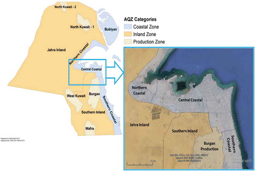
Air quality zones (AQZs) were designated under the UNDP KIEMS project as shown in Figure 2 (Freeman et al., 2016).

Figure 2. Proposed Kuwait air quality zones (Freeman et al., 2016).

As mentioned earlier, the use of the 99% Rule method raises a concern as to whether residents within air zones that meet KAAQS standards are protected from high air pollutant concentration exposure to the same extent as residents within an air zone that meets standards under the “3-Strike” method. Determining an effective classification method is important given the many subpopulation groups (SPGs) in Kuwait due to the large concentration of expatriate workers and family members. Li et al. (2008) recognized the uncertainties associated with setting fixed ambient air standards and used a fuzzy Monte Carlo analysis method to evaluate different variables to establish optimum ranges for specific SPGs (Li et al., 2008). While this method recognizes individual sensitivities, it is impractical to implement from a national air management perspective. For our method, the ambient standard is assumed to be a static limit.

Exposure estimation and Monte Carlo methodology

Health impacts caused by hazardous air pollutants, both cancerous and noncancerous, are due in part to the exposure of a receptor to the pollutants. Estimating the exposure, however, is not alone sufficient to measure risk. Estimating the actual dose a receptor is subject to over a given time and concentration provides a more complete evaluation of risk, even though it does not include the toxicity of the chemicals involved. By comparing the different air quality classification methods against a pollutant that already has an ambient air quality standard, we can assume the toxicity impacts have already been accounted for and remove this element from our evaluation. Our approach in evaluating relative risk based on dosage from different classification methods can also be applied to the many hazardous air pollutants (HAPs) that do not have ambient air quality standards or clinical trial results.

Estimating individual exposures based on ambient monitoring is prone to risk and uncertainty (Pernigotti et al., 2013; Thunis et al., 2013). The ambient monitoring station is assumed to measure air concentrations for the same population. Variations in wind speed and direction have a tremendous impact on who gets exposed and who does not (Pratt et al., 2012). Additionally, lifestyle of the population, construction of houses and workspaces, and exposure duration have major impacts on overall exposure (Bell, 2006).

Uncertainty in exposure estimates based on air dispersion models has long been recognized and accepted by regulatory agencies (Colvile et al., 2002; Fox, 1984). When exposure concentrations are calculated, the results are usually given as a time-weighted average (hourly, daily, or annual) that is then multiplied by the appropriate time period to get the duration exposure amount (Zhang and Batterman, 2013). Using a Monte Carlo analysis (MCA) based on the air concentration probability distribution, each hour can be randomly sampled over the course of the duration period and summed to create a range of possible exposures. MCA has been used for several exposure studies to account for the wide variability of exposures (Gerharz et al., 2013; Tan et al., 2014).

The U.S. EPA Human Health Risk Assessment (HHRA) method defines the chronic daily intake (CDI) (or average daily dose) of chemicals through inhalation in vapor phase using the following equation:

(1)

where C is the concentration of the air pollutant (μg/m³), IR is the inhalation rate (given as 20 m³/day for adults), EF is the exposure frequency (days/year), ED is the exposure duration (years), BW is body weight (kg), and AT is averaging time (usually 365 days/year) (EPA, 2005b). The CDI calculates a value measured in μg/kg_BW-day, where kg_BW is body weight in kilograms. CDI is normally multiplied by the cancer slope factor (CSF) of a carcinogenic chemical for a target organ in order to calculate the incremental excess lifetime cancer risk (IELCR) or divided by a reference dose (RfD) of a noncarcinogenic chemical to get the hazard quotient. Dosage was used for comparison in this study instead of mortality because Kuwait has a highly mobile population and large expatriate community that does not live in the country for more than 3 years. Other studies that looked as mortality assumed a highly stable population (Sanhueza et al., 2010). Also, as mentioned previously, not incorporating the toxicological values of chemicals (CSF or RfD) allows our method to be used for the many chemicals that do not have accepted studies.

Pollutant concentrations can be calculated with different methods. These include city-wide averaging (CWA), which takes the average of all monitor readings within a region or zone; nearest monitoring (NM), which assigns the concentration measured at the closest station to a receptor; inverse distance weighting (IDW), which calculates a concentration by assigning a weighting factor to readings from all monitors based on the inverse of the distance of that station to the receptor; and ordinary Kriging (OK), which assigns a more complex weighting factor to all monitors in a region or zone based on the assumption that the unknown concentration between two stations is a random variable (Rivera-González et al., 2015). The NM method is used in this paper, whereby we assume that all populations near the monitoring station are exposed to the same concentration of the pollutant at the same time. Previous studies showed that indoor/outdoor air concentration ratios were ≥1, showing that higher pollutant concentrations occur indoors (Schembari et al., 2013) or in vehicles (Abi-Esber and El-Fadel, 2013). For our method, we assumed individuals are exposed to the same hourly concentration value throughout the analysis period, whether they are indoors or outdoors.

In order to facilitate the MCA, a new concentration duration factor (CDF) is defined where CDF = C × EF × ED, allowing eq 1 to be rewritten as

(2)

The value of the CDF factor is measured in μg-hr/m³. The actual concentration (C) of a pollutant in the air, the duration of exposure (ED) to that concentration, and then number of times the concentration exceeds standards (EF) are independent variables that can be fitted with a probability distribution to allow predictive analysis (Lonati et al., 2011). Georgoupolos and Seinfeld (1982) used histograms to determine frequency of concentrations, assuming ergodic samples taken from independent and identical distributions (Georgopoulos and Seinfeld, 1982). This concept was used by Sharma et al. (2013) to fit probability distribution functions (PDFs) to measured air monitoring data using goodness-of-fit statistics to select appropriate distributions (Sharma et al., 2013).

Hourly concentration data from air monitoring stations were used to calculate the CDF using the assumption that an air monitoring station measures the exposure of the local population. In order to create a model to compare the different classification methods, actual monitoring station data for different pollutants from 2008 to 2010 were collected and plotted as frequency distributions to create composite distributions to represent a typical year. PDFs were fitted to the distribution curves using @RISK 7.0.0 Industrial Edition (Palisades Software; Palisades, 2015). The same software was used to later run the MCA based on the calculated PDFs. Distributions for annual concentrations for O₃, NO₂, and SO₂ ranged in terms of Weibull, log-normal, and beta distributions. These results were consistent with similar distributions found in the literature (Lu, 2003; Morel et al., 1999; Noor et al., 2011).

To compare possible CDI exposures to a pollutant, the overall ambient air quality was assumed to be in compliance with the KAAQS based on the individual classification method. The exposure duration was set to 3 years, which required three individual 3-Strike classifications but only one 99% Rule classification. For the 3-Strike method, a maximum number of three exceedances per year was enforced, while for the 99% Rule, there was no fixed number of exceedances per year other than the maximum number for 3 years.

Two different comparison cases are made in this study. In the first case, only one monitoring station was evaluated in order to compare the two methods at the simplest level. In the second case, three monitoring stations in the same zone were evaluated. Hourly concentration measurements from 2008 to 2010 of O₃ and NO₂ were selected as test pollutants due to the availability of reliable data from the three stations.

Single station case

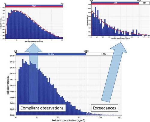
Each pollutant data set was divided into compliance and exceedance measurements by creating two PDFs—one for concentration readings under the standard (Compliance) and one for readings that exceed the standard (Exceedances), as shown in Figure 3. PDFs of the measured data were selected based the Akaike information criteria (AIC), Bayesian information criteria (BIC), and Anderson–Darling (A-D) statistics generated during the fitting (Palisades, 2015). The PDF having the best agreement among the two statistics was chosen to represent the component data.

Figure 3. Breakdown of 8-hr O₃ concentrations into compliance and exceedance distributions.

The individual PDFs were then used in a Monte Carlo analysis based on the individual hours of each method over 3 years of monitoring data (26,280 hours total). The individual hours for each method in the single station run are shown in Table 3.

Table 3. Single station run exposure hours for compliance and exceedance concentrations.

	Classification method
	3-Strike	99%
Compliance hours	26,271	26,017
Exceedance hours	9	263

Total pollutant concentration exposure was calculated by summing the randomly drawn values from each method over the number of individual hours as shown here:

(3)

where CDF is the total concentration exposure over 3 years for a particular classification method in g-hr/m³, N is the total number of compliance hours for a particular classification method, M is the total number of exceedance hours allowed for a particular classification method (note that N + M = 26,280 hr), A_hr is the independent variable sampled from the compliance PDF for 1-hr concentration in g-hr/m³, and X_hr is the independent variable sampled from the exceedance PDF for 1-hr concentration in g-hr/m³.

Other assumptions were made for the remaining variables of eq 1. The body weight variable (BW) is normally evaluated at 70 kg for adults (EPA, 2005b); however, the average body mass for Kuwait has increased over the years and is on par with the United States and other Western nations. Using 2014 census data from the Kuwait Central Statistics Bureau and assuming non-Kuwaiti residents from different national groups have the same average weights described by other researchers (Walpole et al., 2012), Kuwait has a composite average body of mass 66.4 kg as shown in Table 4. Age and gender are not considered.

Table 4. Composite weight of adults in Kuwait.

Nationality groups	Average body mass (kg) (Walpole et al., 2012)	Population (CSB, 2014)	Percent population	Average body mass component (kg)
Kuwait	80.7	1,191,234	32.60%	26.3
Asia	57.7	1,525,083	41.70%	24
Africa	60.7	73,300	2.00%	1.2
North America	80.7	18,297	0.50%	0.4
Europe(*)	70.8	13,966	0.40%	0.3
World(**)	62	837,372	22.90%	14.2
	Total	3,659,252	100.00%	66.4

*Includes residents from South American, Central American, Australia, and European countries.

**Includes residents from Arab and nonspecified countries.

The final variable, inhalation rate (IR), is given an average value of 15.2 m³/day for adults by the U.S. EPA (EPA, 2005b). Other studies have used lower average values such as 13.1 m³/day to account for reduced rates during sleeping and sedentary activities (Marshall et al., 2006). The higher, more conservative average rate of 15.2 m³/day was used for this study.

Applying the Central Limit Theorem

Because the samples are taken randomly and independently from the PDFs, the Central Limit Theorem (CLT) was used to simplify the calculation process, resulting in normal distributions (N) for the total exposure where

(4)

and

(5)

given that μ₁ and μ₂ are the arithmetic means of the compliance and exceedance PDFs, respectively, and σ₁ and σ₂ are the standard deviations of the PDFs (Ott and Mage, 1981).

Calculations

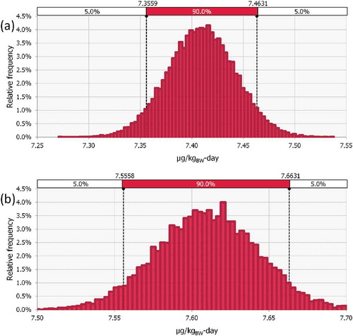
A Monte Carlo analysis was run for 10,000 iterations for the composite CDI values based on normal distribution-based compliance and exceedance PDFs. Figure 4 shows the CDI distributions of 8-hr O₃ for both the 3-Strike and 99% Method models.

Figure 4. Composite model distributions of CDIs for the (a) 3 Strike method and (b) 99% Rule method.

Statistical tests

To compare the results of the run, a null hypothesis (H_o) assumed that there was no significant statistical difference (p < 0.05) between the mean and variance of the CDI for both methods. Accepting the null hypothesis means that either method could be used without concern that exposure was overly high in method. Rejecting the null hypothesis would show that there were statistically significant differences (p < 0.05) between the mean and variance of the two methods and that one method had higher exposure risk.

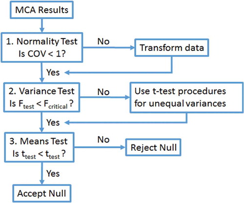
Since the CLT is used, distributions are assumed to be normal, however a coefficient of variation (COV) test is used to confirm normality, where COV = σ/μ. If the COV is less than unity, then the PDF can be considered normal (Abdi, 2010). If the COV > 1 and the PDF is a nonnormal distribution, data transformation can be performed to convert the data to a normal distribution such as using a log transformation or Box–Cox transformation (Osborne, 2010).

Variance testing can then use the one-sided F-test where the F-statistic is defined as

(6)

where σ_3-Strike is the standard deviation of the 3-Strike method CDI MCA and σ_99% is the standard deviation of the 99% Rule method MCA. In each case, the degrees of freedom (df) are n – 1, or 26,279, giving a critical value of F, F_c(.05, 26,729) = 1.02. If the F test passes and variances are assumed to be equal, the means can be tested with a standard t-test in which the test statistic t_* is defined as

(7)

where μ_3-Strike is the mean of the 3-Strike method CDI MCA, μ_99% is the mean of the 99% Rule method MCA, and SE_diff is the standard error of the difference, defined as

(8)

where the sample size n is equal for both groups. The df is again 26,729, making the t critical, t_c(0.05, 26729) = 1.645.

With such a large sample size, however, the low critical value of the F statistic may cause the variance test to fail. For unequal variances, a modified t-test for unequal variances (Satterthwaite t-test) is used (Ruxton, 2006). The Satterthwaite t-test is similar to eqs 7 and 8 except an approximate degree of freedom value is calculated to calibrate the Satterthwaite t statistic with normal t statistic values. The new Satterthwaite degrees of freedom (df_s) is calculated by

(9)

which reduces to

(10)

If the means test fails, then the null hypothesis is rejected. A summary of the hypothesis testing procedure is shown in Figure 5.

Figure 5. Flow chart of hypothesis testing procedures for single station case.

Multiple station case

For multiple stations, a process is followed similar to that for the single station case with some modifications. An assumption is made that each station is independent from each other and therefore does not observe the same concentration. Based on this assumption, the probability of one station having a noncompliant (NC) observation is therefore independent at the time of the observation. Because we are assuming the zone is in compliance, we know that the maximum allowable NC observation to stay in compliance is a constant for each classification method. We can initially assume that each station has an equal number of NC observations required to meet the classification limit. For the 3-Strike method, each station is assumed to have 3 NC observations, and for the 99% Rule method, each station has 268 NC observations. However, because we are looking at exposure potential, we have to assume that some stations will have more NC observations than others. In a worst-case scenario for the 99% Rule, one station could have all NC observations while the other stations have no exceedances and the zone could still be in compliance. A more likely scenario is that some stations will have more NC observations than others. To account for local exposure at individual stations, additional NC hours are added to each station based on the estimated percentage of NC observations over the 3 years (%NC). For each NC hour added, a compliant hour is removed, in order to keep the total number of observation hours constant. A binomial distribution is used to model the number of additional NC hours with the number of trials. Input values for a binomial distribution include the number of trials, n, and the continuous success probability, p (Palisades, 2015). If m is the number of years of observation (in our case, 3 years), then for the 3-Strike method, n = 3 × (m – 1), and for the 99% Rule method, n = 268 × (m – 1). The continuous success probability for each station, p_i, is calculated for each station using the following method:

Step 1. Determine %NC over the three years for each station.

(11)

Step 2. Sum the individual %NC’s and normalize each station’s p_i.

(12)

Step 3. Estimate the number of NC hours and residual compliance (RC) hours at each station for each method.

(13)

Step 4. Run the MCA with CFD’s for each method and for each station similar to eq 4:

(14)

where

• μ_Ai is the mean of the compliance observations PDF at station_i multiplied by the number of compliance hours for the method being evaluated.

• σ_Ai is the standard deviation of the compliance observations PDF at station_i multiplied by the square root of the number of compliance hours for the method being evaluated.

• μ_Xi is the mean of the noncompliant observations PDF multiplied by NC_i hours for the method being evaluated.

• σ_Xi is the standard deviation of the non-compliant observations PDF multiplied by the square root of the NC_i hours for the method being evaluated.

• μ_Ari is the mean of the compliance observations PDF at station_i multiplied by the RC_i hours for the method being evaluated.

• σ_ARi is the standard deviation of the compliance observations PDF at station_i multiplied by the square root of the RC_i hours for the method being evaluated.

The CDI is then calculated for each station and each method using the same process as the single station case. The multiple station case also uses the same statistical tests as the single station case.

Results

Single station case

Models were prepared to compute the CDI values for 1-hr NO₂ and 8-hr O₃ from an air monitoring station located in a coastal urban area and used data collected between 2008 and 2010. The particular station was located in a dense residential area on a government building approximately 300 m away from a major highway. The resulting PDFs estimated from the data sets and related air quality standards are shown in Table 5.

Table 5. Representative PDFs for single station case.

Pollutant	Air quality standard (μg/m^3)	Compliance PDF distribution	Exceedance PDF distribution
1-hr NO2	200	Gamma	Pareto
8-hr O3	100	Kumaraswamy	Pareto

The PDF means and standard deviations (SD) were then used as input parameters for Normal distributions after applying sample modifications per eq 5. A summary of the inputs (means and standard deviations) for each model are shown in Table 6.

Table 6. Summary of normal distribution input parameters used to calculate CDFs for the single station case (in g-hr/m³).

		Compliance PDF		Exceedance PDF
Pollutant	Method	Mean	SD	Mean	SD
1-hr NO2	3 Strike	1,838,596.79	5,991.89	2,427.8	299.6
	99%	1,820,820.40	5,962.85	70,945.8	1,619.5
8-hr O3	3 Strike	849,524.12	3,750.43	1,106.1	86.7
	99%	841,310.53	3,732.25	32,323.8	468.5

The CDIs computed through the MCA of each pollutant using samples drawn from compliance and exceedance distributions in Table 6 are shown in Table 7.

Table 7. Single station CDIs (in μg/kg_BW-day).

Pollutant	Method	Mean	SD
1-hr NO2	3 Strike	16.04	0.05
	99%	16.48	0.05
	Difference	2.7%
8-hr O3	3 Strike	7.41	0.03
	99%	7.61	0.03
	Difference	2.7%

Statistical testing of the single station case for 1-hr NO₂ is shown in Table 8.

Table 8. Statistical testing for single station CDI case for 1 hr NO₂.

Method	3 Strike	99%
COV	0.003	0.003
Ftest	1.059
df	26,279	26,279
Fcritical (p < 0.05)	1.02
Result (Ftest < Fcritical)	FALSE
ttest	955.73
dfs	52,514
tcritical (p < 0.05)	1.664
Result (ttest < tcriticial)	FALSE

For the 1-hr NO₂, the COVs of both methods are much less than 1 indicating the samples most likely came from normal distributions. As predicted in the Methods section, the large number of samples caused the variance test to fail. Using a modified t-test with unequal variances and a computed degrees of freedom approximation, the test for means also fails, requiring us to reject the null hypothesis and accept that there are significant statistical differences between the two method for 1-hr NO₂ classification. Critical values for the F and t-tests were calculated using the F-distribution and t-distribution quantile functions, respectively, in R (R Core Team, 2015).

Statistical testing results for the single station case of 8 hr O₃ is shown in Table 9.

Table 9. Statistical testing for single station CDI case for 8 hr O₃.

Method	3 Strike	99%
COV	0.004	0.004
Ftest	1.005
df	26,279	26,279
Fcritical (p < 0.05)	1.02
Result (Ftest < Fcriticial)	TRUE
ttest	701.7
df	52,560
tcritical (p < 0.05)	1.664
Result (ttest < tcritical)	FALSE

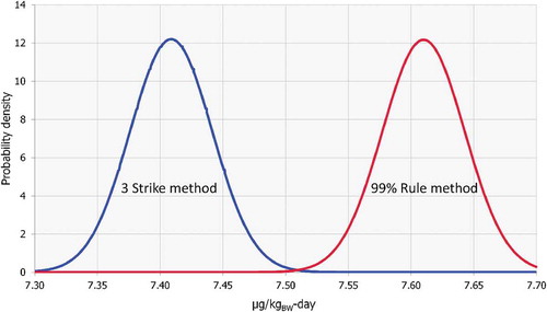
As with the 1-hr NO₂, the 8-hr O₃ shows that the null hypothesis must be rejected, despite the passing of the variance test and being 2.7% different. For single stations, the 3 Strike method offers less exposure over the same duration than the 99% Rule method. A more graphical representation of the two CDIs is shown in Figure 6 where the different CDI distributions for 8-hr O₃ are plotted together, showing the difference in means. This assumes that BW and IR are constant.

Figure 6. Comparison of CDI distributions for 8-hr O₃.

Results for multiple station case: 1-hr NO₂

Three stations within a coastal zone of Kuwait were selected for comparison with 3 years of data for 2008–2010. In addition to the station used for the single case, two stations located in nearby residential areas were also used. In each case the stations were mounted on the roofs of government buildings. The steps described above in eqs 11 through 14 were used to determine the weighted %NC probability of continuous success, p, for the binomial distributions used to estimate additional noncompliant days. A summary of initial station parameters is shown in Table 10, including number of compliant and NC hours, the binomial probability, and the base PDF distribution forms used for the MCA.

Table 10. Parameters for multiple station case of 1-hr NO₂.

Parameters	AMS 1	AMS 2	AMS 3	Total
Compliant hours	25,780	26,230	25,684	77,694
NC hours	524	74	620	1,218
%NC	1.99%	0.28%	2.36%	4.63%
p (from eq 12)	43.0%	6.1%	50.9%	100%
Compliant PDF distribution	Gamma	Weibull	Triangle
NC PDF distribution	Pareto	Kumaraswamy	Lognormal

The parameters of Table 10 were used to define the normal distributions used in the MCA for each method as summarized in Table 11.

Table 11. Normal distribution inputs for multiple station case CDFs of 1-hr NO₂.

	3-Strike method (g-hr/m^3)
	AMS 1	AMS 2	AMS 3
Compliant normal distributions
Mean	1,838,597	1,001,779	1,751,400
SD	5,991.9	4,907.7	7640.7
NC normal distribution
Mean	2,427.80	2,024.86	2,447.45
SD	299.58	77.37	444.99
	99% Rule method (g-hr/m^3)
	AMS 1	AMS 2	AMS 3
Compliant normal distributions
Mean	1,802,162	974,065	1,705,873
SD	6,133.6	4,880.3	7,557.3
NC normal distribution
Mean	216,883.59	180,887.22	218,638.96
SD	2,831.51	731.23	4,205.88

The resulting descriptive statistics for the CDIs of each station after 10,000 iterations during the MCA are shown in Table 12.

Table 12. CDI statistics for multiple stations of 1-hr NO₂.

	AMS 1	AMS 2	AMS 3
Mean (μg/kgBW-day)
3-Strike method	16.03	8.73	15.27
99% Rule method	17.06	9.24	16.29
Difference	6.4%	5.8%	6.7%
SD (μg/kgBW-day)
3-Strike method	0.05	0.04	0.07
99% Rule method	0.06	0.04	0.08

The statistical tests for the methods at each station are shown in Table 13 for 1-hr NO₂. As with the single station, the multiple stations pass the normality and variance tests, but fails the mean tests. The null hypothesis is thus rejected for the multiple stations case for 1-hr NO₂.

Table 13. Statistical tests for multiple stations of 1-hr NO₂.

	AMS 1	AMS 2	AMS 3
Normality testing
3-Strike method COV	0.003	0.005	0.004
99% Rule method COV	0.004	0.005	0.005
Variance testing
Ftest	0.75	0.947	0.769
df	26,279	26,279	26,279
Fcritical (p < 0.05)	1.02	1.02	1.02
Result (Ftest < Fcritical)	TRUE	TRUE	TRUE
Means testing
ttest	3175.0	1919.3	2484.4
df	52,560	52,560	52,560
tcritical (p < 0.05)	1.644	1.644	1.644
Result (ttest < tcritical)	FALSE	FALSE	FALSE

Results for multiple station case: 8-hr O₃

The multiple station case for 8-hr O₃ follows the same procedure as the 1-hr NO₂. Table 14 shows the input parameters. Table 15 shows the normal distribution inputs used for CDF in the MCA. Table 16 summarizes the input statistics of the computed CDIs, and Table 17 shows the statistical test results.

Table 14. Parameters for multiple station case of 8-hr O₃.

Parameters	AMS 1	AMS 2	AMS 3	Total
Compliant hours	25,048	24,653	25,151	74,852
NC hours	699	566	72	1,337
%NC	2.71%	2.24%	0.29%	5.24%
p (from eq 12)	51.8%	42.8%	5.4%
Compliant PDF distribution	Kumaraswamy	Kumaraswamy	Kumaraswamy
Exceedance PDF distribution	Pareto	Exponential	Pareto

Table 15. Normal distribution inputs for multiple station case CDFs of 8-hr O₃.

	3-Strike method (μg-hr/m3)
	AMS 1	AMS 2	AMS 3
Compliant normal distributions
Mean	849,524.1	964,430.5	597,880.3
SD	3,750.4	3,529.2	2,465.7
NC normal distribution
Mean	844.1	775.1	483.5
SD	138.0	112.4	60.4
	99% Rule method (μg-hr/m3)
	AMS 1	AMS 2	AMS 3
Compliant normal distributions
Mean	825,548.10	988,490.08	722,209.16
SD	3,707.63	3,682.44	3,025.70
NC normal distribution
Mean	75,399.3	69,252.4	40,748.6
SD	1,299.1	1,058.3	368.3

Table 16. CDI statistics for multiple stations of 8-hr O₃.

	AMS 1	AMS 2	AMS 3
Mean (μg/kgBW-day)
3-Strike method	7.4	8.4	5.21
99% Rule method	7.85	9.21	6.65
Difference	6.1%	9.6%	27.6%
SD (μg/kgBW-day)
3-Strike method	0.033	0.031	0.021
99% Rule method	0.034	0.033	0.027

Table 17. Statistical tests for multiple stations of 8-hr O₃.

	AMS 1	AMS 2	AMS 3
Normality test
3-Strike COV	0.004	0.004	0.004
99% Rule COV	0.004	0.004	0.004
Variance test
Ftest	0.905	0.844	0.655
df	26,279	26,279	26,279
Fcritical (p < 0.05)	1.02	1.02	1.02
Result (Ftest < Fcritical)	TRUE	TRUE	TRUE
Means test
ttest	1532.48	2900.33	6829.69
df	52,560	52,560	52,560
tcritical (p < 0.05)	1.664	1.664	1.664
Result (ttest < tcritical)	FALSE	FALSE	FALSE

The 8-hr O₃ passes the test for normality and variance, but fails the test for equal means. Again, the null hypothesis is rejected, showing that there is a statistically significant difference between the CDI of the two methods.

Conclusion

This study presents a new approach for evaluating air quality zone classification methods by breaking the distribution of historical pollution concentration into compliance and exceedance concentration PDFs. This approach allows the distribution of historical data from an air monitoring station to create ambient air quality profiles to test different compliance scenarios. Two different cases were used to test the methods—a single station case where the data of only one station was used, and a multiple station case where two or more stations’ data are used. In the multiple station case example, three stations were used. Statistical methods were defined to determine normality of the distributions used for the CDI, and whether the different methods had statistically similar variances and means.

A null hypothesis was proposed that stated the variance and means of both methods were not significantly different and could therefore be used based on non-statistically based preferences. Rejecting the null showed that the methods did indeed have enough statistically significant differences that to choose one method over another would result in higher local exposure over the duration period.

Using a Monte Carlo analysis, it was shown that the two methods do indeed have statistically significant differences in their variances and means for the pollutants tested (NO₂ and O₃). While the null hypothesis is rejected, the individual methods are not. The large sample size and degrees of freedom can reject null hypothesizes due to extreme sensitivity in variances. Using a different approach based on effect size, in which the population size does not affect the statistic, the methods can be compared with better merit. Because the COV tests showed that the distributions were strongly normal in nature, making the mean and SD strong descriptive statistics that cannot be discounted. The choice of statistic used to compare the classification methods, the CDI, represents a relative risk of exposure, and not a risk of disease, injury, or damage.

Choosing to use one classification method over the other may involve other non-health-related factors besides comparing CDI of chemicals. Other factors may include availability of air monitoring data, economic impacts of declaring a zone noncompliant and the ability of the local air management authority to enforce an improvement program. Other reasons may be that the zone is sparsely populated such as a hydrocarbon production field or an inland desert that may not need the same level of exposure protection. Also areas experiencing rapid growth would constantly be in noncompliance under a strict 3-Strike method based classification whereas a 99% Rule method would average some of the emission increases over time and look at the overall trend. Recommendations for using both methods are shown in Table 18.

Table 18. Recommended uses for classification methods.

3-Strike method	99% Rule method
One station in zone	Multiple stations in zone
Zone is primarily residential	Zone is primarily industrial or sparsely populated
Incomplete or data sets less than 12 months	Several years of data available
Static development	Changes in development and land uses

The fact that one method of classification may cause higher exposure than another is not a reason to reject its use, but to use it with discretion.

Acknowledgment

This work was completed under the United Nations Development Program’s Kuwait Integrated Environmental Management System project from 2011 to 2014.

Funding

The authors would like to acknowledge the financial support of the Natural Science and Engineering Research Council of Canada (NSERC), the Mathematics of Information Technology and Complex Systems (MITACS), and Lakes Environmental.

Additional information

Funding

The authors would like to acknowledge the financial support of the Natural Science and Engineering Research Council of Canada (NSERC), the Mathematics of Information Technology and Complex Systems (MITACS), and Lakes Environmental.

Notes on contributors

Brian Freeman

Brian Freeman, was the Team Leader, Air Regulatory Management Systems for the UNDP KIEMS project, and is currently in the Ph.D. program at the School of Engineering at the University of Guelph, Canada.

Ed McBean

Ed McBean, Ph.D., is a Professor of Environmental Engineering in the School of Engineering at the University of Guelph, Canada.

Bahram Gharabaghi

Bahram Gharabaghi, Ph.D., is a Professor of Environmental Engineering in the School of Engineering at the University of Guelph, Canada.

Jesse Thé

Jesse Thé, Ph.D., is a Professor of Mechanical Engineering at the University of Waterloo, Canada and the President of Lakes Environmental.

References

- Abdi, H. 2010. Coefficient of variation. In Encyclopedia of Research Design, ed. N. Salkind, 5. London, UK: Sage.
- Abi-Esber, L., and M. El-Fadel. 2013. Indoor to outdoor air quality associations with self-pollution implications inside passenger car cabins. Atmos. Environ. 81:450–63. doi:10.1016/j.atmosenv.2013.09.040
- Bell, M.L. 2006. The use of ambient air quality modeling to estimate individual and population exposure for human health research: A case study of ozone in the Northern Georgia Region of the United States. Environ. Int. 32:586–93. doi:10.1016/j.envint.2006.01.005
- Bermudez, R.M., and P.M. Fine. 2010. South Coast Air Quality Management District 5 Year Network Assessment, 94. South Coast Air Quality Management District. https://www3.epa.gov/ttnamti1/files/networkplans/CASCAQMDassess2010.pdf (accessed January 25, 2017).
- California Air Resources Board. 2013. Air monitoring site list generator. In Air Quality and Meteorological Information System, ed. R. Bhullar. http://www.arb.ca.gov/qaweb/sitelist_create.php (accessed January 25, 2017).
- Central Statistical Bureau, Kuwait. 2014. Statistics of transportation, trade, agriculture and transport. Kuwait City, Kuwait: Central Statistical Bureau.
- CIA. 2015. The World Factbook—Kuwait. http://www.epa.gov/airtrends/pm.html (accessed January 25, 2017).
- Cohen, J., T. Fitz-Simons, and M. Wayland. 1999. Guideline on Data Handling Conventions for the PM NAAQS. Research Triangle Park, NC: U.S. EPA.
- Colvile, R.N., N.K. Woodfield, D.J. Carruthers, B.E.A. Fisher, A. Rickard, S. Neville, and A. Hughes. 2002. Uncertainty in dispersion modelling and urban air quality mapping. Environ. Sci. Policy 5:207–20. doi:10.1016/S1462-9011(02)00039-4
- Crosman, E.T., and J.D. Horel. 2010. Sea and lake breezes: A review of numerical studies. Boundary-Layer Meteorol. 137:1–29. doi:10.1007/s10546-010-9517-9
- Cuxart, J., M.A. Jiménez, M. Telišman Prtenjak, and B. Grisogono. 2014. Study of a sea-breeze case through momentum, temperature, and turbulence budgets. J. Appl. Meteorol. Climatol. 53:2589–609. doi:10.1175/JAMC-D-14-0007.1
- European Economic Community. 1980. Council Directive 80/779/EEC of 15 July 1980 on air quality limit values and guide values for sulphur dioxide and suspended particulates. European Economic Community.http://eur-lex.europa.eu/legal-content/EN/TXT/PDF/?uri=CELEX:31980L0779&from=EN (accessed January 25, 2017).
- European Union. 2008. Ambient air quality and cleaner air for Europe, 2008/50/EC. Off. J. Eur. Union. http://eur-lex.europa.eu/legal-content/EN/TXT/PDF/?uri=CELEX:32008L0050&from=en (accessed January 25, 2017).
- Fox, D.G. 1984. Uncertainty in air quality modeling. Bull. Am. Meteorol. Soc. 65:27–36. doi:10.1175/1520-0477(1984)065<0027:UIAQM>2.0.CO;2
- Freeman, B., B. Gharabaghi, J. Thé, M. Munshed, S. Faisal, M. Abdullah, and A.A. Aseed. 2016. Mapping air quality zones for coastal urban centers. J. Air Waste Manage. (In press) doi:10.1080/10962247.2016.1265025
- Georgopoulos, P.G., and J.H. Seinfeld. 1982. Statistical distributions of air pollutant concentrations. Environ. Sci. Technol. 16:401A–16A. doi:10.1021/es00101a002
- Gerharz, L.E., O. Klemm, A.V. Broich, and E. Pebesma. 2013. Spatio-temporal modelling of individual exposure to air pollution and its uncertainty. Atmos. Environ. 64:56–65. doi:10.1016/j.atmosenv.2012.09.069
- KAMCO. 2013. State of Kuwait: Economic & financial facts. KIPCO Asset Management Company KSC. http://www.kamconline.com/Temp/Reports/48218661-476e-43f1-8d12-ecc124e90e93.pdf (accessed January 25, 2017).
- Kuwait Environmental Public Authority. 2012. Amendment to provisions in Decision 210/2001 (articles 76 and 79), 1073. Kuwait City, Kuwait: Kuwait Al Yom.
- Li, H.L., G.H. Huang, and Y. Zou. 2008. An integrated fuzzy-stochastic modeling approach for assessing health-impact risk from air pollution. Stochastic Environ. Res. Risk Assess. 22:789–803.doi:10.1007/s00477-007-0187-1
- Lonati, G., S. Cernuschi, and M. Giugliano. 2011. The duration of PM10 concentration in a large metropolitan area. Atmos. Environ. 45:137–46.doi:10.1016/j.atmosenv.2010.09.033
- Lu, H.-C. 2003. Comparisons of statistical characteristic of air pollutants in taiwan by frequency distribution. J. Air Waste Manage. 53:608–16. doi:10.1080/10473289.2003.10466194
- Lubkert-Alcamo, B. 1994. The update and revision of the 1987 WHO Air Quality Guidelines. Pollut. Atmos. 4232:7.
- Marshall, J.D., P.W. Granvold, A.S. Hoats, T.E. McKone, E. Deakin, and W.W. Nazaroff. 2006. Inhalation intake of ambient air pollution in California’s South Coast Air Basin. Atmos. Environ. 40:4381–92. doi:10.1016/j.atmosenv.2006.03.034
- Marshall, J.D., E. Nethery, and M. Brauer. 2008. Within-urban variability in ambient air pollution: Comparison of estimation methods. Atmos. Environ. 42:1359–69. doi:10.1016/j.atmosenv.2007.08.012
- McCabe, J.G. 2015. Area designation for the 2015 Ozone National Ambient Air Quality Standards. Washington, DC: U.S. EPA.
- Morel, B., S. Yeh, and L. Cifuentes. 1999. Statistical distributions for air pollution applied to the study of the particulate problem in Santiago. Atmos. Environ. 33:2575–85. doi:10.1016/S1352-2310(98)00380-X
- Murray, D.R., and M.B. Newman. 2014. Probability analyses of combining background concentrations with model-predicted concentrations. J. Air Waste Manage. Assoc. 64:248–54. doi:10.1080/10962247.2013.846282
- Noor, N.M., C.-y. Tan, N.A. Ramli, A.S. Yahaya, and N.F.F.M. Yusof. 2011. Assessment of various probability distributions to model pm10 concentration for industrialized area in peninsula Malaysia: A case study in Shah Alam and Nilai. Aust. J. Basic Appl. Sci. 5:2796–811.
- Osborne, J.W. 2010. Improving your data transformations: Applying the Box–Cox transformation. Practical Assess. Res. Eval. 15(12):1–9.
- Ott, W.R., and D.T. Mage. 1981. Measuring air quality levels inexpensively at multiple locations by random sampling. J. Air Pollut. Control Assoc. 31:365–69. doi:10.1080/00022470.1981.10465230
- Palisades. 2015. @RISK User’s Guide—Risk Analysis and Simulation Add-In for Microsoft® Excel. Ithaca, NY: Palisades Corporation.
- Pan, X., and P. Lee. 2009. California State and Local Air Monitoring Network Plan. Sacramento, CA California Environmental Protection Agency.
- Pernigotti, D., M. Gerboles, C.A. Belis, and P. Thunis. 2013. Model quality objectives based on measurement uncertainty. Part II: NO2 and PM10. Atmos. Environ. 79:869–78. doi:10.1016/j.atmosenv.2013.07.045
- Pratt, G.C., M. Dymond, K. Ellickson, and J. The. 2012. Validation of a novel air toxic risk model with air monitoring. Risk Anal. 32(1):96–112.
- R Core Team. 2015. R: A Language and Environment for Statistical Computing, 3.1.3. Vienna, Austria: R Foundation for Statistical Computing.
- Rivera-González, L.O., Z. Zhang, B.N. Sánchez, K. Zhang, D.G. Brown, L. Rojas-Bracho, A. Osornio-Vargas, F. Vadillo-Ortega, and M.S. O’Neill. 2015. An assessment of air pollutant exposure methods in Mexico City, Mexico. J. Air Waste Manage. Assoc. 65:581–91. doi:10.1080/10962247.2015.1020974
- Ruxton, G.D. 2006. The unequal variance t-test is an underused alternative to Student’s t-test and the Mann–Whitney U test. Behav. Ecol. 17:688–90. doi:10.1093/beheco/ark016
- Sanhueza, P., J. Pizarro, C, Vargas, M. Torreblanca, and M. Passalacqua. 2010. Health risk estimation due to carbon monoxide pollution at different spatial levels in Santiago, Chile. Environ. Monit. Assess. 167:165–73. doi:10.1007/s10661-009-1039-x
- Schembari, A., M. Triguero-Mas, A.D. Nazelle, P. Dadvand, M. Vrijheid, M. Cirach, D. Martinez, F. Figueras, X. Querol, X. Basagaña, M. Eeftens, K. Meliefste, and M.J. Nieuwenhuijsen. 2013. Personal, indoor and outdoor air pollution levels among pregnant women. Atmos. Environ. 64:287–95. doi:10.1016/j.atmosenv.2012.09.053
- Sharma, P., P. Sharma, S. Jain, and P. Kumar. 2013. An integrated statistical approach for evaluating the exceedence of criteria pollutants in the ambient air of megacity Delhi. Atmos. Environ. 70:7–17. doi:10.1016/j.atmosenv.2013.01.004
- South Coast Air Quality Management District. 2010. Introduction to the South Coast Air Quality Management District, 2. Diamond Bar, CA: South Coast Air Quality Management District.
- Tan, Y., A.L. Robinson, and A.A. Presto. 2014. Quantifying uncertainties in pollutant mapping studies using the Monte Carlo method. Atmos. Environ. 99:333–40. doi:10.1016/j.atmosenv.2014.10.003
- Thunis, P., D. Pernigotti, and M. Gerboles. 2013. Model quality objectives based on measurement uncertainty. Part I: Ozone. Atmos. Environ. 79:861–68. doi:10.1016/j.atmosenv.2013.05.018
- U.S. Environmental Protection Agency. 1970. National Ambient Air Quality Standards (NAAQS), 40 CFR part 50. Fed. Reg. https://www.law.cornell.edu/cfr/text/40/part-50 (accessed January 25, 2017).
- U.S. Environmental Protection Agency. 1991. Designation of areas for air quality planning purposes. 40CFR81. https://www.law.cornell.edu/cfr/text/40/part-81 (accessed January 25, 2017).
- U.S. Environmental Protection Agency. 2005a. An Explanation of EPA’s Nine-Factor Analysis, Technical support document for December 17, 2004 designations. https://www3.epa.gov/pmdesignations/1997standards/documents/final/TSD/Ch5.pdf (accessed January 25, 2017).
- U.S. Environmental Protection Agency. 2005b. Human Health Risk Assessment Protocol for Hazardous Waste Combustion Facilities, 1284. Washington, DC: Office of Solid Waste and Emergency Response. https://epa-prgs.ornl.gov/radionuclides/2005_HHRAP.pdf (accessed March 22, 2017).
- U.S. Environmental Protection Agency. 2007. Clean Air Act, Operating Schedules. 40 CFR 58.12. https://www.gpo.gov/fdsys/granule/CFR-2014-title40-vol6/CFR-2014-title40-vol6-sec58-12/content-detail.html (accessed January 25, 2017).
- U.S. Environmental Protection Agency. 2016a. National Ambient Air Quality Standards (NAAQS). https://www.epa.gov/criteria-air-pollutants/naaqs-table (accessed January 25, 2017).
- U.S. Environmental Protection Agency. 2016b. National Area and County-Level Multi-Pollutant Information, Green Book Nonattainment Areas. U.S. EPA. https://www.epa.gov/green-book/green-book-national-area-and-county-level-multi-pollutant-information (accessed January 25, 2017).
- Walpole, S.C., D. Prieto-Merino, P. Edwards, J. Cleland, G. Stevens, and J. Roberts. 2012. The weight of nations: An estimation of adult human biomass. BMC Public Health 12:1–6. doi:10.1186/1471-2458-12-439
- World Health Organization. 2006. WHO Air Quality Guidelines for Particulate Matter, Ozone, Nitrogen Dioxide and Sulfur Dioxide. Global Update 2005. Summary of Risk Assessment. Geneva, Switzerland: World Health Organization.
- Zhang, K., and S. Batterman. 2013. Air pollution and health risks due to vehicle traffic. Sci. Total Environ. 450–51:307–16. doi:10.1016/j.scitotenv.2013.01.074