Mapping air quality zones for coastal urban centers

ABSTRACT

This study presents a new method that incorporates modern air dispersion models allowing local terrain and land–sea breeze effects to be considered along with political and natural boundaries for more accurate mapping of air quality zones (AQZs) for coastal urban centers. This method uses local coastal wind patterns and key urban air pollution sources in each zone to more accurately calculate air pollutant concentration statistics. The new approach distributes virtual air pollution sources within each small grid cell of an area of interest and analyzes a puff dispersion model for a full year’s worth of 1-hr prognostic weather data. The difference of wind patterns in coastal and inland areas creates significantly different skewness (S) and kurtosis (K) statistics for the annually averaged pollutant concentrations at ground level receptor points for each grid cell. Plotting the S-K data highlights grouping of sources predominantly impacted by coastal winds versus inland winds. The application of the new method is demonstrated through a case study for the nation of Kuwait by developing new AQZs to support local air management programs. The zone boundaries established by the S-K method were validated by comparing MM5 and WRF prognostic meteorological weather data used in the air dispersion modeling, a support vector machine classifier was trained to compare results with the graphical classification method, and final zones were compared with data collected from Earth observation satellites to confirm locations of high-exposure-risk areas. The resulting AQZs are more accurate and support efficient management strategies for air quality compliance targets effected by local coastal microclimates.

Implications: A novel method to determine air quality zones in coastal urban areas is introduced using skewness (S) and kurtosis (K) statistics calculated from grid concentrations results of air dispersion models. The method identifies land–sea breeze effects that can be used to manage local air quality in areas of similar microclimates.

Introduction

The use of air quality zones (AQZs) as a tool for air management was identified as early as the 1960s (Breivogel et al., 1961; Holland et al., 1960) and was first mandated for State Implementation Plans (SIPs) under the U.S. Clean Air Act (CAA) of 1990 (U.S. Environmental Protection Agency [EPA], 1990). In the United States, AQZs are based on designated air quality control regions (AQCRs) that include defined municipalities and groups of intrastate and interstate counties (40CFR81, 1991). Currently there are 264 designated AQCRs with 121 in some form of noncompliance (or nonattainment) with the National Ambient Air Quality Standards (NAAQS; EPA, 2016). In general, AQZs describe areas where air pollutants are below ambient standards (“in attainment” or “in compliance”), or exceeding them (“in nonattainment” or “in noncompliance”). The U.S. Environmental Protection Agency (EPA) uses ambient air monitoring data measured by county to determine nonattainment areas (Carr and Yan, 2012). The EPA initially required states to identify zones of nonattainment for 8-hr ozone. These regulatory requirements later included sulfur dioxide, particulate matter less than 10 µm (PM₁₀), and particulate matter less than 2.5 µm (PM_2.5). A consequence of these regulations was the installation of thousands of monitoring stations throughout the United States. In 2014, 1,293 active ozone monitoring stations were in operation at areas considered to be at risk (EPA, 2015). Despite the widespread placement of monitoring equipment, designation of AQZs (or AQCRs) is limited to areas defined by county lines (Carr and Yan, 2012).

The European Union initiated a zone management system for its member states in 2008 with Directive 2008/50/EC (European Community [EC], 2008). In addition to designated AQZs, the directive requires at least one monitor for PM_2.5 in every 100,000 km². Low emission zones (LEZs) were established in more than 200 European cities that enforced restrictions on cars and heavy-duty vehicles (Holman et al., 2015). The drawback of LEZs is that the zones were established based on city boundaries and not on geophysical features (Henschel et al., 2013).

Turkey followed the European Directive to define AQZs for eight different regional areas within its 81 provinces (CYGM, 2010). The process used multiple methods and tools, including statistical analysis of monitoring station historical data, use of geodatabases and Geographic Information System (GIS) evaluations, air dispersion and local sources, and meteorological effects (Karaca, 2012). Furthermore, the Turkish evaluation only employed average daily values of pollutants, instead of hourly averages, with daily values discarded if more than 30% of hourly data was unavailable.

China established Control Zones in 1995 that covered over 11.4% of its territory to manage ever-increasing levels of SO₂ (Hao et al., 2000). Additional “Acid Rain Control Zones” covered almost 8.4% of China. Zones were established based on local meteorological, topographical, and soil conditions that had low pH (acidic). Other designation factors included precipitation pH values and ambient SO₂ measurements.

Coastal urban centers

Approximately 40% of the population of the United States (more than 100 million people) live in coastal shoreline counties (National Oceanic and Atmospheric Administration [NOAA], 2013). An estimate of the world population living in coastal areas was approximately 1.4 billion people in 2015, with expected populations growing to more than 1.6 billion by 2024 (Geohive, 2015). With the growth of coastal communities comes air management challenges (Gamas et al., 2015). Local ambient air quality is impacted by the volume of emissions from industry, transportation, and residential activities, as well as meteorological and seasonal changes (Fiore et al., 2015; Kimbrough et al., 2013). Coastal zones are also subject to land–sea breezes (LSBs), caused by the diurnal differential heating/cooling of the sea and land (Crosman and Horel, 2010; Cuxart et al., 2014; Tsai et al., 2011). LSBs continuously shift direction and speed up over the course of the day, sometimes extending as deep as 150 km inland depending on topography, and even deeper for desert regions (Miao et al., 2015; Zhu and Atkinson, 2004).

Variables that impact the extent and intensity of LSBs are largely geophysical, and include surface heat flux, wind patterns, atmospheric stability and moisture, dimensions of local water bodies, shoreline curvature, topography, and surface roughness (Crosman and Horel, 2010; Lu and Turco, 1995). These shifting winds recirculate emissions, which have negative impacts for coastal communities (Lu and Turco, 1996). Modeling and evaluating the impact of this recirculation have been the subjects of several studies (Crosman and Horel, 2010; Levy et al., 2009; Wu et al., 2013; Zhu and Atkinson, 2004). A key objective of this study is to determine the extent of LSBs along a developed coastline using a quantitative method that incorporates multiyear weather patterns.

Statistical approaches to evaluating LSBs have been applied by many researchers. Levy et al. (2009) developed a spatiotemporal model to evaluate mesoscale recirculation using a Regional Atmospheric Modeling System Hybrid Particle and Concentration Transport (RAMS-HYPACT) modeling system and inert particles. They used the recirculation potential index (R) to measure recirculation potential at each grid cell. The R index is a ratio of the wind’s vector and scalar sums over a 24-hr period. A low numerical R index indicates a constantly changing wind direction, while a high value indicates constant wind direction during the time. Existing sources were used for model inputs, and results were compared to readings from more than 26 air monitoring station distributed throughout the area of evaluation.

Wu et al. (2013) also used an R index to identify LSB impacts, as well as a ventilation index (VI) based on wind speeds at different altitudes. Both Levy and Wu required measurements at different altitude using radio soundings or balloons to capture vertical wind speeds (Wu et al., 2013). Neither team’s findings were incorporated into air zone management. In addition to Levy and Wu, several studies effectively used neural networks and other machine learning-based techniques to analyze complex dispersion patterns in coastal areas (Elangasinghe et al., 2014; Feng et al., 2015), but these methods require large data sets for training.

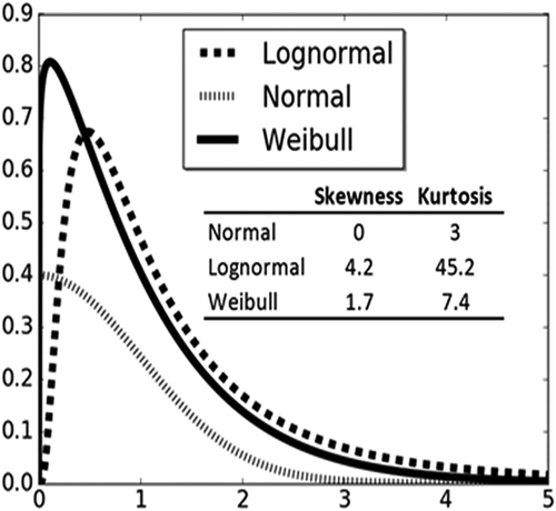
Classifying categories based on higher order moments, such as skewness (S) and kurtosis (K) statistics, was applied by Martins as early as 1965 to discriminate between beach and dune sand grains (Martins, 1965). Other fields have more recently used S-K statistics for pattern recognition (Crosilla et al., 2013), medical recovery (Chi-Chun et al., 2008), and music genre classification (Seo and Lee, 2011). Skewness (S) is a third-order moment around the sample mean that measures the symmetry (or asymmetry) of the sample’s distribution. A normal distribution has S = 0. Kurtosis (K) is a fourth-order moment that measures the peakness of a distribution relative to a normal distribution. A normal distribution has a K = 3. A highly skewed distribution with a high kurtosis will have a sharp peak and a long tail on one side of the mean (National Institute of Standards and Technology [NIST], 2016). The general equations for each statistic are

(1)

(2)

where x is an individual data point, is the data mean, σ is the standard deviation, and N is the number of data points (Cristelli et al., 2012). Some kurtosis formulas apply a correction term of “–3” to eq 2 (called excess kurtosis) in order to bias the equation to obtain K = 0 for a normal distribution. Kurtosis may also be calculated as

(3)

The first term, , is approximately 1/N for large values of N (N > 200), thus reducing eq 3 to eq 2 (Cox, 2010). Difference of distributions with various S and K values are shown in Figure 1.

Figure 1. Distributions representing various S and K statistics.

Using higher order moments amplifies the error of the sample points from the sample mean and as variance to allow better classification (Seo and Lee, 2011). Crosilla et al. (2013) applied S and K statistics to remote sensor images in order to group terrain into homogeneous categories based on data sets collected from light detection and ranging (LiDAR). Alberghi et al. (2002) used kurtosis to identify vertical velocity components in convective boundary layers associated with LSBs. They used both measured data and data from air dispersion models to identify correlation between Skewness and Kurtosis (Alberghi et al., 2002). This is very similar to our requirement, in which we seek to classify areas of similar wind fields among two separate categories—inland and coastal. While multiple parameters impact the overall mixing and distribution of pollutant concentrations, our hypothesis assumes that long-term pollutant concentrations in coastal regions can be categorized using S-K statistics from inland regions due to the high frequency of multidirectional winds compared to the high frequency of prevailing winds in inland regions. This assumption is based on previously stated examples in the literature, and is further demonstrated by our modeling approach. Observed data collected from earth observation satellites validate our assumptions.

Our other hypothesis is that identification of LSB areas can be used to establish AQZs. AQZ determination methods mentioned previously did not take terrain and local weather patterns into consideration to establish zones, even though meteorological impacts have long been recognized as key contributors to air management planning (Leavitt, 1960). Using existing political borders for air zones is convenient when a state or county is small. A larger jurisdiction may have different terrain, land use, features, and microclimates that lead to unequal ambient exposures for receiving populations. Basing AQZ boundaries strictly on existing political boundaries penalizes stakeholders located outside heavily polluted areas but inside the designated zone (Carr and Yan, 2012). One way to incorporate local terrain and weather patterns into the AQZ designation process is to use modern air dispersion models that utilize terrain and weather as input parameters to generate spatial pollutant concentration distributions (Ghannam and El-Fadel, 2013b; Irwin, 2014).

Materials and methods

A simple method to estimate LSB extent is a key component to proposing defined air quality zones suitable for compliance enforcement for countries that have a significant industrial and population presence on or near coastlines. This study presents a novel approach that incorporates LSB into the zone designation process, employing air dispersion modeling results from virtual sources placed in high-risk receptor areas. A virtual source with the same emission parameters was placed at several designated areas of concern and modeled using a dispersion model over several individual years. The resulting dispersion patterns over a 20 km 20 km grid with the virtual source at the center was converted to a histogram and descriptive statistics were calculated. The S and K statistics were used to classify individual areas as inland wind effect impacted or coastal wind effect impacted.

The methodology is summarized here:

1. Scope the overall area, accounting for coast, terrain, and land use.

2. Identify high-risk receptor areas.

3. Model dispersion of by a common virtual sources at selected risk areas over 1 yr (8,760 hr) for multiple years.

4. Compute S-K statistics for individual years.

5. Determine coastal/inland classification based on majority of runs at each site.

The following subsections illustrate the new approach as applied by the United Nations Development Program (UNDP) Kuwait Integrated Environmental Management System Project to support the definition of AQZs in Kuwait (Freeman et al., 2013).

Modeling land–sea breeze patterns

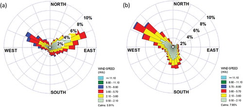
LSBs are the primary dispersal agent of generated emissions for sources located near the sea (Cuxart et al., 2014). Coastal areas often contain large concentrations of people and industries, thus making them sensitive receptor areas. In Kuwait, the overwhelming majority of people and industry are located in coastal areas. The first step of the process is to determine how far LSB patterns encroach inland. The diurnal nature of LSB is particularly strong for countries in the study area (Zhu and Atkinson, 2004). Effects also vary seasonally, with the sea breezes lasting longer in the summer months than in the winter months. Zhu and Atkinson (2004) reported maximum penetration along the Persian Gulf coast countries of sea breezes in excess of 250 km. Of the multiple variables reported by Conklin, Zhu suggests that the main factors affecting LSB are the land–sea heat flux, ambient wind patterns, and local topography. Figure 2 displays examples of coastal wind distributions for southern Kuwait captured at ground level by an air monitoring station. Similar patterns showing wind directions distributed around the compass with a prevailing component are common for coastal areas (Lozano et al., 2013).

Figure 2. (a) Typical daytime and (b) nighttime ground-level LSB winds in southern Kuwait for the year 2011.

Puff modeling of virtual urban air pollution sources

This new AQZ delineation methodology requires investigation to assess how far inland coastal effect winds travel, by evaluating wind patterns throughout the area. Virtual emission sources were placed in areas considered to have high receptor and source risks. These included dense residential areas, industrial zones, and concentrated urban environments. The same virtual source is inserted at each site in order to compare the dispersion patterns over the same time frames. Source parameters were selected to represent typical industrial operations and published sources (Chusai et al., 2012). Table 1 contains parameters used for each virtual source configuration. The source was designed to represent a typical boiler burning high-sulfur diesel fuel.

Table 1. Puff model virtual source properties.

Parameter	Value
Modeling period	January 1, 2009–December 31, 2011
Averaging period	8,760 hr
Emission rate, SO2	200 kg/hr
Stack height	20 m
Stack internal diameter	1 m
Gas exit velocity	30 m/sec
Gas exit temperature	1000 K

Air dispersion patterns were modeled using CALPUFF 5.8.4 and CALMET 5.8.4 (EPA, 2014) set to 1 km 1 km receptor grids in a 20 km 20 km area at ground level for a total of 400 points per run. CALMET can accommodate the complex wind fields associated with coastal environments and has been used for modeling land–sea breezes for other similar flat terrain (Mangia et al., 2010). Lakes Environmental generated the mesoscale numerical weather prediction (NWP) model (MM5) data to compute wind fields for three individual years (2009 to 2011). The model calculated the annual average (8,760 hours) for each year at each virtual source location.

CALPUFF was chosen because it is a nonsteady puff model that calculates complex wind fields typically found in coastal zones (Ghannam and El-Fadel, 2013a; Indumati et al., 2009; EPA, 2014; Weiss et al., 2014). Digitized local terrain and geophysical data were incorporated into the process during the development of the CALMET model using the Terrain Elevation Data Processing (TERREL), and other preprocessors (Scire et al., 2000). Digital terrain files were downloaded from the Shuttle Radar Topography Mission (SRTM3) Global Coverage (~90 m) Version 2 database (U.S. Geological Survey [USGS], 2000). The Global Land Cover Characteristics (GLCC) database maintained by the U.S. Geological Survey (USGS) provided land use data (USGS, 2008). Coastline features were further processed using shoreline data from the Global Self-consistent, Hierarchical, High-resolution Shoreline Database (GSHHS) provided by the National Oceanic and Atmospheric Administration (NOAA) National Centers for Environmental Information (NOAA, 2015). Default values were used for other settings.

Sulfur dioxide (SO₂) was use as a pollutant for the virtual sources due to the extensive data already collected by local air monitoring stations and heavy use of sulfur rich fuels in local combustion processes (Al-Awadhi, 2014; Al-Rashidi et al., 2005). SO₂ was also used for other studies involving air control zones (Hao et al., 2000; Henschel et al., 2013; Pereira et al., 2007). While photochemistry is an important process in secondary formation of pollutants, it is not important to the evaluation of dispersion and recirculation of pollutants in the AQZ. Therefore, this study did not consider it as part of the modeling.

Prognostic weather setup

MM5 is a limited-area, nonhydrostatic, terrain-following sigma-coordinate model designed to simulate or predict mesoscale atmospheric circulation, developed by Pennsylvania State University (PSU) and National Center for Atmospheric Research (NCAR) (Grell et al., 1994). It is used widely for generating local wind fields and weather data for air dispersion models (Ghannam and El-Fadel, 2013a; Lee et al., 2009; Tsai et al., 2011; Zhu and Atkinson, 2004). Zhu and Atkins (2004) evaluated observed and modeled weather conditions at Kuwait International Airport and reported good results for daily and monthly observations using MM5 data. The 100 100 km data for the study years were prepared in 4-km cells. Vertical layers for the wind fields were calculated at 0, 20, 40, 80, 160, 320, 640, 1200, 2000, 3000, and 4000 m. Concentration results from the air dispersion modeling were analyzed using StatTools and @RISK 7.1 Industrial Edition (Palisade, 2013) to generate histograms and comparative statistics.

Case study site description

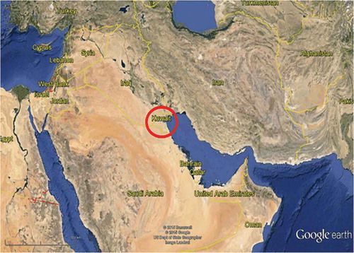
Kuwait is a small country of approximately 17,818 km² located on the northwest corner of the Persian Gulf, between 46.56 and 48.37 ºE and between 28.51 and 30.16 ºN with more than 499 km of coastline (CIA, 2015). The country is classified as a desert zone, with the highest altitude reaching only 300 m above sea level. In 2011, approximately 3.1 million people lived in Kuwait (Central Statistic Bureau [CSB], 2012) with over 64% of its annual gross domestic product (GDP) coming from the production of hydrocarbons (KAMCO, 2013). Other industries in Kuwait include power generation and water desalination using heavy oil and natural gas at five sites, steel making using electrical induction furnaces, and food preparation. The country has more than 6,600 km of paved roads and more than 1.8 million cars in service (OICA [International Organization of Motor Vehicle Manufacturers], 2014). Kuwait has 6 governorates divided into 81 districts. Figure 3 shows the map of Kuwait and its location in the Persian Gulf region. Recent studies demonstrate that air quality has deteriorated along the Kuwaiti coastline, where most of the population is clustered (Al-Awadhi, 2014). The resulting concern from local citizens has led to protests and negative press coverage (Carlisle, 2010).

Figure 3. Location of Kuwait.

Results and discussion

Air dispersion model results and histograms

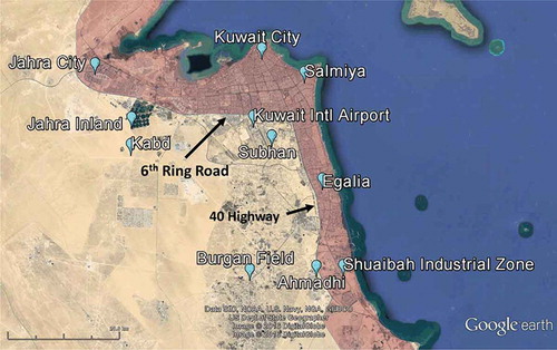
Virtual sources were placed at key areas to represent different risk areas within Kuwait. The selected sites include industrial and urban areas, as well as oil production and remote desert areas. These sites are distributed among the main industrial and living areas to reflect the main land uses in Kuwait: mainly industrial, residential, oil production, and open desert. The sites are listed in Table 2 and shown in Figure 4. A partial 10-km coastal buffer is also shown in Figure 4 that incorporates two major roads running north/south (40 Highway) and east/west (6th Ring Road).

Table 2. Virtual site locations.

Location	Longitude	Latitude	Comments
Ahmadhi	48.0915º	28.9933º	Dense heavy industrial area
Burgan Field	47.9644º	28.9879º	Oil production operations
Egalia	48.1032º	29.1393º	Dense residential area
Jahra City	47.6671º	29.3321º	Dense urban area
Jahra Inland	47.7378º	29.2418º	Sparse population
Kuwait City	47.9874º	29.3580º	Dense urban area
Kabd	47.7366º	29.1967º	Sparse population
Kuwait Intl Airport	47.9710º	29.2440º	Sparse population
Salmiya	48.069º	29.3180º	Dense residential area
Shuaibah Industrial Zone	48.1428º	28.9944º	Dense heavy industrial are
Subhan	48.0064º	29.2113º	Dense heavy industrial area

Figure 4. Location of virtual sources for air dispersion analysis shown with partial 10-km buffer and main perimeter roads.

Figure 5 displays examples of individual ground level concentration outputs from the virtual SO₂ sources described in Table 1, while Figure 6 shows histograms of the SO₂ concentrations calculated by the model to show the distribution of concentrations within the model area. Concentration color gradients were plotted on the same scale for comparison purposes. The model is based only on runs accomplished with SO₂ over an annual average of 8,760 hours.

Figure 5. Ground-level air dispersion patterns from inland and coastal virtual SO₂ sources averaged over 8,760 hr (annual): (a) Jahra Inland dispersion (inland), year 2010; (b) Kuwait City dispersion (coastal), year 2009.

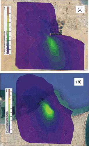
Figure 6. Histograms of ground level concentrations from inland and coastal virtual SO₂ sources averaged over 8,760 hr (annual): (a) Jahra Inland histogram (inland), year 2010; (b) Kuwait City histogram (coastal), year 2009.

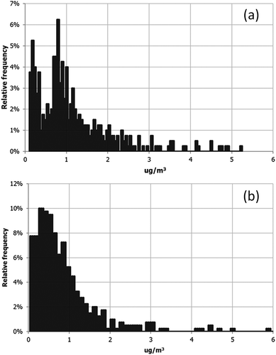
Different studies using ambient air measurements over time have assumed normal distributions of measurements and included statistics such as the mean and standard deviation (Henschel et al., 2013; Rivera-González et al., 2015; Suresh and Desa, 2005). For highly skewed data sets, traditional statistics cannot effectively describe the distribution. As described in the introduction section, skewness and kurtosis best describe the different concentration values generated by the puff highly skewed dispersion model runs.

Zones were identified in Kuwait visually at first in order to establish baseline results. The calculated statistics for each site and annual run are shown in Table 3 along with distance to shore. The runs properly classified as inland (S < 3, K < 20) or coastal (S > 3, K > 20) are classified as strong. Most of the misclassified runs using the S-K method are sites that are clearly situated in an inland or coastal area but are not properly classified (a site in an inland area classified as coastal and vice versa). The Shuaibah Industrial Zone–year 2010 is located 2.1 km from the coast and is considered coastal due to its physical location and because 2 out of 3 trials classified the zone as coastal. Figure 7 plots the skewness versus kurtosis values from Table 3. The Subhan site is 9.3 km from the coast and near the border of a coastal zone and a production zone. The Kabd site is clearly inland (16.8 km from the coast), but shows many coastal wind pattern features, suggesting that the LSB effect extends deeply into this region of Kuwait due to the flat topography and relatively smooth surfaces existing as a result of limited development.

Table 3. Skewness and kurtosis statistics for virtual sites.

Site	Zone	Year	Skewness		Kurtosis	Distance (km)
Ahmadhi	Coastal	2009	4.18		30.98	7.1
		2010	4.00		25.43
		2011	4.37		30.13
Burgan Field	Inland	2009	1.84		8.32	19.2
		2010	2.34		11.11
		2011	2.74		13.47
Egalia	Coastal	2009	8.16		115.40	2.7
		2010	7.33		94.55
		2011	6.74		77.61
Jahra City	Coastal	2009	5.07		48.94	4.9
		2010	4.38		37.47
		2011	6.46		70.95
Jahra Inland	Inland	2009	1.74		6.52	12.7
		2010	2.15		9.26
		2011	2.29		9.31
Kabd	Inland	2009	2.89		12.96	16.8
		2010	3.19		16.33
		2011	3.55		18.85
Kuwait City	Coastal	2009	4.71		32.72	2.2
		2010	4.45		30.18
		2011	5.22		41.33
Kuwait Intl Airport	Inland	2009	1.88		9.98	11.9
		2010	1.56		6.56
		2011	2.77		16.23
Salmiya	Coastal	2009	5.19		40.12	2.2
		2010	5.76		48.53
		2011	9.17		123.69
Shuaibah Industrial Zone	Coastal	2009	3.08		22.59	2.1
		2010	2.33		12.56
		2011	3.29		22.87
Subhan	Coastal	2009	2.80		12.06	9.3
		2010	3.02		13.07
		2011	3.68		26.72

Note. Misclassified sites are italicized.

Figure 7. S-K plot of virtual sources in Kuwait.

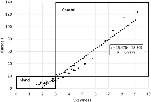
Regions are highlighted showing inland classification areas (orange) and coastal (blue). A linear trend line of the plotted points, K = 11.901S – 15.732, shows strong correlation (R² = 0.943).

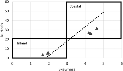
To confirm the procedure, random points were modeled in the nearby nation of Qatar. An inland point was taken at Abu Naklah Air Base (ANAB, 25.1208 °E /51.3177 °N) and a coastal point taken at Masaeed Industrial City (MIC, 24.9911 °E/51.5506 °N) for the same years (2009–2011) using the same virtual source parameters as shown in Table 2. The points are approximately 570 km south-southeast from Kuwait International Airport.

The methodology properly classified each location as inland and coastal. The S-K points are shown in Figure 8, along with a trend line using the parameters from Figure 7.

Figure 8. S-K plot of virtual sources in Qatar.

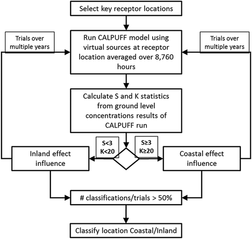
Figure 9 contains a flowchart that summarizes the process to develop this coastal/inland determination. The process requires at least three trial years to allow a majority winner-take-all classification if one year returns a misclassification.

Figure 9. Coastal/inland determination process flow chart.

Identifying air quality zones for Kuwait

The delineation and categorization of the AQZs for Kuwait was completed to assign appropriate control technologies to local air emission processes in order to improve air quality in zones that did not meet air quality standards and prevent deterioration in zones that did (Carr and Yan, 2012). This approach assumes that areas with predominantly coastal effect winds have different exposure risks than areas with predominantly inland winds, and that they should therefore be managed differently. In Kuwait, most of the population, industries, power generation, and downstream hydrocarbon processes are located within 10 km of the coast. The Bay of Kuwait is a relatively shallow body of water that never exceeds a depth of 20 m. Seasonal surface water temperatures vary from 12.4ºC to 34.8ºC (Al-Mutairi et al., 2014). The presence of this body of water provides a significant source of energy that impacts local weather patterns (Mizak et al., 2007; Panin and Foken, 2005).

After coastal effect limits were estimated using the S-K method, zones were further defined by incorporating existing roads and expressways. Where practical, these physical features were taken into account to allow for easier management. These features included major highways, political divisions, and security fences protecting hydrocarbon production areas. As a result, the coastal/inland boundaries follow a main Kuwaiti ring road up to the northeast end of Kuwait Bay. Municipal district boundaries were also used to promote familiarity when transitional areas were close to estimated boundaries. The major oil fields were also separately identified as zones due to security concerns. The final AQZs are shown in Figure 10.

Figure 10. Kuwait air quality zones.

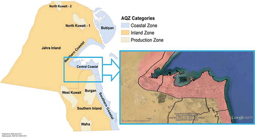
The pink area in Figure 10 shows the buffer area from Figure 4, and the dark border show final zone borders. Statistics for the air quality zones are shown in Table 4.

Table 4. Air quality zone statistics.

Item	Zone	Zone Type	Area	Percent of total land	Population (2005)	Percent of total population
			km^2
1	Northern Coastal	Coastal	365	2.10%	392,598	11.50%
2	Southern Coastal	Coastal	796	4.60%	737,997	21.60%
3	Central Coastal	Coastal	426	2.50%	2,280,773	66.70%
4	Bubiyan	Coastal	847	4.90%	NA
5	Southern Inland	Inland	2,700	15.60%	NA
6	Jahra Inland	Inland	10,556	61.00%	9,205	0.30%
7	Wafra	Production	269	1.60%	NA
8	West Kuwait	Production	375	2.20%	NA
9	North Kuwait 1	Production	267	1.50%	NA
10	North Kuwait 2	Production	105	0.60%	NA
11	Burgan	Production	592	3.40%	NA
	Total		17,298	100%	3,420,573	100%

The Kuwaiti coastal air zones include 14.1% of the land area and 99.8% of the population. The inland zones include 76.6% of the land area and the production zones represent 9.3%. Descriptions of the individual zone types are provided here:

• Coastal zones. The four coastal zones also include Bubiyan Island and the smaller islands off the coast of Kuwait, including Failaka and Kubar Islands. While comprising only 9.2% of the land area, coastal zones are home to 99.7% of all people living and working in Kuwait. More than 88% of people live in the Southern and Central zones alone. With additional construction of residential areas and industrial facilities, these are the primary zones for air quality management.

• Inland zones. The two inland zones are mostly farms, camping areas, military base, and free range land, comprising more than 76% of the land area in Kuwait. The area is sparsely populated (0.3% of the population).

• Production zones. Designated oil and gas fields operated by the national oil companies require different compliance activities due to their industrial processes and site security. Production zones were established to allow the oil industry to apply their own regulatory program under local regulatory guidance and supervision. The zones follow the fencelines of the secure areas and represent more than 9.3% of the land area with no residential population and a sparsely distributed work force. Additionally, larger production zones were found to have internal microclimates compared to the neighboring inland zones during the modeling phase. This is due in large part to overgrazing by herd animals outside the secured areas. The resulting change in land cover clearly impacts albedo and surface heat capacity. Perimeters around production zones are fenced and provide a continuous boundary.

Validation of methodologies

In addition to applying the method to a secondary area in Qatar, three different methodologies were used to test the validity of the model and the final AQZ selection. The first test was a comparison of prognostic weather data sets to determine whether the air dispersion model component is robust. The second test used a support vector machine (SVM) to classify the data sets and compare to the less computationally intensive method we presented. The final test evaluated the regions identified as a result of the LSB classification against satellite-based data.

Prognostic weather data comparison between MM5 and WRF

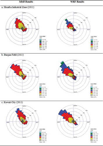
Another common option for prognostic weather data is the Weather Research and Forecasting (WRF) model also developed by NCAR (Skamarock et al., 2008). WRF has been used in the region for different climatology studies looking at wind forecasts for different applications (Amjad et al., 2015). Direct comparisons of the two models, MM5 and WRF, show that the results are statistically similar, with topography playing a large role in predictive accuracy (Gsella et al., 2014; Henmi, 2004). Comparing ground-level wind patterns generated by both the MM5 and WRF models over a common 100 100 km area using 4-km grid cells, we found that wind directions were very similar, with wind fields approximately 10% higher for the MM5 results. When applied to the CALPUFF model, the lower WRF wind speeds provided higher ground-level concentrations; however, the final results support our method using MM5. Wind roses for three locations are shown in Figure 11.

Figure 11. Comparison of wind patterns using MM5 and WRF prognostic data.

Classification by SVM

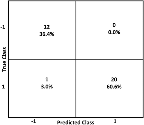
SVMs are a class of supervised-learning-based models that classify input data sets by mapping into high-dimensional feature spaces. While SVMs have been used since 1995 (Cortes and Vapnik, 1995), they have only relatively recently been applied to air pollution concentration predictions (Lu and Wang, 2005; Luna et al., 2014; Moazami et al., 2016). A full description of the SVM is beyond the scope of this paper, but several excellent references and online tutorials are available. A linear SVM was trained with the data set in Table 3 using the Classification Learner module in MATLAB 2015a with a linear kernel function (Yang et al., 2011). The input data was standardized by the software prior to training. Inland classification was converted to –1 while coastal classification was designated with 1. The SVM was initially trained only with S and K results. The resulting confusion matrix (Figure 12) could achieve an overall accuracy of 87.9%—comparable to the results of graphing the S and K values.

Figure 12. Confusion matrix of trained SVM with S and K inputs.

The use of the SVM allows additional features to be included so that multiple inputs can be used to improve accuracy. Adding the coastal distance improved overall accuracy to 97%, as shown in Figure 13. The trained SVM was tested using the Qatar data set and achieved 100% accuracy.

Figure 13. Confusion matrix of trained SVM with S, K, and distance to coast inputs.

Satellite validation of mixing areas

In order to evaluate the effectiveness of the new zone boundaries, satellite-derived data from NASA’s Ozone Monitoring Instrument (OMI) on the Aura satellite was obtained and mapped for NO₂ over 46.125–49.125 ºE and 28.375–30.375 ºN (Boersma et al., 2011; Strawa et al., 2013). NO₂ was used to map actual concentrations due to the higher concentrations measured in Kuwait by the OMI sensor instead of SO₂. This provided higher contrast of readings for visual analysis. Ground monitoring stations have also confirmed that SO₂ concentrations are not significant, while concentrations of NO₂ are (Al-Awadhi, 2014).

Data were downloaded from the Giovanni web based system (Acker and Leptoukh, 2007) and converted to Excel spreadsheets. The data resolution from the OMI was limited to 0.25 degrees per cell, representing approximately 312 km². In addition, the data represented the average measurement of a vertical column extending from the surface of the planet to the satellite sensor in a sun-synchronous orbit approximately 705 km above sea level. The satellite repeats its orbit every 16 days (OMI, 2012).

Annual averages and standard deviations for NO₂ (measured in 10¹⁵ molecules/cm²) for the Kuwait area were plotted as shown in Figures 14 and 15, respectively. Highest concentrations are located on the Central and Southern coasts, corresponding to heavy urban development and industrial activities. The pattern roughly follows the central and southern coastal zones.

Figure 14. Annual concentration of NO₂ in Kuwait for 2011.

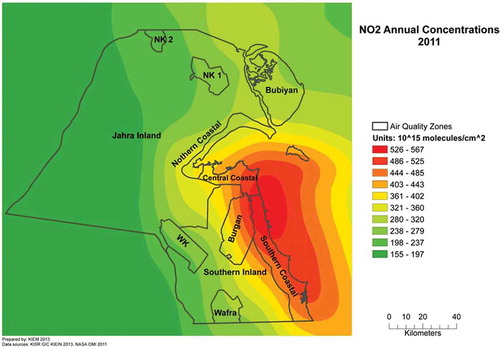
Figure 15. Annual standard deviation of NO₂ concentration as percentage of annual concentration in Kuwait for 2011.

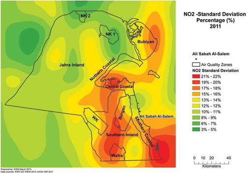
Annual average concentrations of NO₂ show that the highest concentrations are clustered on the coast. Other zones may contribute to the ambient concentration, but exposure risks are predominately located in the Central and Southern coastal zone areas. Looking at the standard deviation of the annual average NO₂ concentrations shows that different areas vary at different rates throughout the year. Areas of high variance occur in the Central coast and Southern inland zones, while the Southern coastal zone stays relatively constant. A zone with high ambient concentrations that does not fluctuate has higher exposure risk.

Air quality exposure risk scores

To identify where high-exposure-risk areas are, a risk scoring method was developed that incorporated annual average concentration (μ) and annual concentration variance (σ²). High values of annual concentrations and annual variance were defined as annual concentrations greater than one standard deviation from the mean (> μ + σ) or approximately 1.64 times the mean. This value accounts for the highest 5% of values. Low values were assumed to be less than one standard deviation from the mean (< μ – σ) or approximately 0.836 times the mean.

The following assumptions of risk were used:

1. Areas with high annual concentrations and low annual variation had the most exposure risk due to constant high concentration exposure throughout the year.

2. Areas with high annual average concentrations and high annual variations were also considered to have high exposure risks.

3. Areas with low annual exposure concentrations and high annual variation had moderate exposure risk due to fluctuating concentration levels throughout the year.

4. Areas with low annual exposure concentrations and low annual variation had low risk.

Data sets used for the annual concentration and annual standard deviations were normalized by taking the average of each cell as

(4)

where CN_i,j is the normalized annual concentration value of the cell, C_i,j is the annual concentration value for the cell, and is the average concentration of all cells. A similar procedure was done to normalize the standard deviation of each cell. Risk values ranged from 0 (low) to 1 (high) for concentration and 0 (low) to 0.5 (high) for standard deviation:

(5)

Risk scores are shown in Table 5 and Figure 16. High- and medium-risk areas are predominantly in the coastal areas, with some medium-risk areas extending inland where heavy oil production takes place.

Table 5. Exposure risk scores.

Score	Risk
1.5	High
1
0.5	Medium
0	Low

Figure 16. NO₂ exposure risk based on annual average concentration and standard deviation. Areas of high population are shown as blue dots.

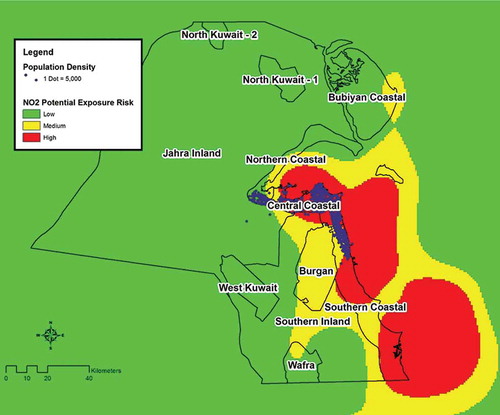
The use of satellite data confirms the high-exposure-risk areas fall within identified AQZs. These areas should have priority in regard to access of pollution control technology and exposure reduction programs. Zones that do not have high exposure risks can be managed differently, such as providing additional control technology for processes in zones near high exposure risk areas to prevent cross-zone transport of emissions.

Conclusion and recommendations

More than 1.4 billion people live in coastal communities where air quality is impacted by complex land–sea breezes. Mapping air quality zones (AQZs) for air quality management in the coastal communities is still done using crude methods based on zones drawn strictly on existing political boundaries. This paper presents a novel statistical risk-based method to identify air quality zones for coastal urban centers that evaluates the effects of local coastal wind patterns and spatial distribution of key urban air pollution sources on air pollutant concentration statistics. This method uses modeled air dispersion results to calculate the skewness and kurtosis (S-K) statistics of air pollutant concentrations by placing virtual air pollution receptors within high-risk gridded population centers of the study area. When graphed against each other, the air quality statistics accurately classify the extent of coastal wind effect within a given zone.

This methodology supports the identification of three distinct air quality zones in Kuwait. These AQZs are tools to classify areas in order to meet local air management strategy. Inland zones were classified to represent primarily desert area with little to no residential populations. Hydrocarbon production zones are included to account for petroleum industry operations taking place in large sections of the study area and managed directly by national oil company assets but supervised by the local regulatory authority. Coastal zones are established that included the majority of residential and industrial areas (roughly 3.4 million people). Once the extent of coastal effect mixing was estimated using the S-K method, geophysical boundaries were approximated to facilitate air quality management.

The model is validated by comparing the concentration and wind data generated using prognostic data with a send weather set. The MM5 and WRF models provided comparable results, especially given the computational differences. Selecting MM5 for the meteorological input to the air dispersion model is validated. The graphical classification approach is tested against a machine learning model. While the support vector machine provided similar and even better results when additional input features are included, the graphical method is a less complicated procedure.

The selection of individual zones is finally validated by comparing satellite data to exposure risk areas. The S-K zone classification method and satellite-based risk evaluation method can be employed by other developing nations with limited air monitoring resources and budgets to identify and establish air quality zones of similar air mixing characteristics.

Additional research is recommended to confirm the application of this method to other areas. Kuwait has relatively homogeneous topography and a very hot climate and is located by a shallow body of water. This method may directly lend itself to other countries in the Persian Gulf region, as shown with sites in Qatar, but should be studied further to evaluate its ability to predict coastal effect mixing for regions with more rugged terrain and more temperate weather.

This study also lends itself to more advanced binary classification methods using ensemble learning techniques. Ensemble learning uses multiple models trained from the same data sets to contribute to the final answer by voting through equal or weighted votes. Binary classification models such as SVMs, linear regression, artificial neural networks, and decision trees can be used together to optimize the identification process by reducing mis-classifications (Narassiguin et al., 2016). LSB classification using ensemble learning will be explored in a future study.

Funding

This work was completed under the United Nations Development Program’s Kuwait Integrated Environmental Management System project from 2011 to 2014. The authors would also like to acknowledge the financial support of the Natural Science and Engineering Research Council of Canada (NSERC), the Mathematics of Information Technology and Complex Systems (MITACS), and Lakes Environmental.

Acknowledgment

Satellite data used in this paper were retrieved from the Giovanni online data system, developed and maintained by the National Aeronautics and Space Administration (NASA), Goddard Earth Sciences (GES) Data, and Information Services Center (DISC).

Additional information

Funding

This work was completed under the United Nations Development Program’s Kuwait Integrated Environmental Management System project from 2011 to 2014. The authors would also like to acknowledge the financial support of the Natural Science and Engineering Research Council of Canada (NSERC), the Mathematics of Information Technology and Complex Systems (MITACS), and Lakes Environmental.

Notes on contributors

Brian Freeman

Brian Freeman was the Team Leader for Air Regulatory Management Systems for the UNDP KIEMS project and is currently in the Ph.D. program at the School of Engineering at the University of Guelph, Canada.

Bahram Gharabaghi

Bahram Gharabaghi, Ph.D., is a Professor of Environmental Engineering in the School of Engineering at the University of Guelph, Canada.

Jesse Thé

Jesse Thé, Ph.D., is a Professor of Mechanical Engineering at the University of Waterloo, Canada, and the President of Lakes Environmental.

Mohammad Munshed

Mohammad Munshed is a developer at Lakes Environmental and a master's student at the University of Waterloo, Canada.

Shah Faisal

Shah Faisal was the Team Leader for Air Information Systems in the UNDP KIEMS project and is currently a project manager for OpenWare, Kuwait.

Meshal Abdullah

Meshal Abdullah was the Team Leader for the Stationary Sources Section in the Department of Air Quality and Follow-Up, Kuwait Public Environment Authority and is currently a master's student in Tohoku University, Japan.

Athari Al Aseed

Athari Al Aseed is a staff member in the Stationary Sources Section in the Department of Air Quality and Follow-Up, Kuwait Public Environment Authority, Kuwait.

References

- 40CFR81. 1991. Designation of areas for air quality planning purposes. Washington, DC: USEPA.
- Acker, J.G., and G. Leptoukh. 2007. Online analysis enhances use of NASA Earth science data. Eos Trans. Am. Geophys. Union 88:4. doi:10.1029/2007EO020003
- Al-Awadhi, J.M. 2014. Measurement of air pollution in Kuwait City using passive samplers. Atmos. Climate Sci. 4:253–71. doi:10.4236/acs.2014.42028
- Al-Mutairi, N., A. Abahussain, and A. El-Battay. 2014. Spatial and temporal characterizations of water quality in Kuwait Bay. Mar. Pollut. Bull. 83:127–31. doi:10.1016/j.marpolbul.2014.04.009
- Al-Rashidi, M.S., V. Nassehi, and R.J. Wakeman. 2005. Investigation of the efficiency of existing air pollution monitoring sites in the state of Kuwait. Environ. Pollut. 138:219–29. doi:10.1016/j.envpol.2005.04.006
- Alberghi, S., A. Maurizi, and F. Tampier. 2002. Relationship between the vertical velocity skewness and kurtosis observed during sea-breeze convection. J. Appl. Meteorol. Climatol. 41:885–889. doi:10.1175/1520-0450(2002)041<0885:RBTVVS>2.0.CO;2
- Amjad, M., Q. Zafar, F. Khan, and M. M. Sheikh. 2015. Evaluation of weather research and forecasting model for the assessment of wind resource over Gharo, Pakistan. Int. J. Climatol. 35:12. doi:10.1002/joc.2015.35.issue-8
- Boersma, K.F., H.J. Eskes, R.J. Dirksen, R.J. van der A, J.P. Veefkind, P. Stammes, V. Huijnen, Q.L. Kleipool, M. Sneep, J. Claas, J. Leitão, A. Richter, Y. Zhou, D. Brunner. 2011. An improved tropospheric NO2 column retrieval algorithm for the ozone monitoring instrument. Atmos. Meas. Technol. 4:1905–28. doi:10.5194/amt-4-1905-2011
- Breivogel, M., S.S. Griswold, A. Hasegawa, and J.R. Taylor. 1961. Air pollution-potential advisory service for industrial zoning cases. J. Air Pollut. Control Assoc. 11:327–35. doi:10.1080/00022470.1961.10468006
- Carlisle, T. 2010. Kuwaiti pupils lead air quality protests. The National, May 2. http://www.thenational.ae/business/kuwaiti-pupils-lead-air-quality-protests (accessed February 3, 2017).
- Carr, D., and W. Yan. 2012. Federal environmental policy and local industrial diversification: The case of the Clean Air Act. Regional Stud. 46:639–49. doi:10.1080/00343404.2010.509131
- Central Statistic Bureau. 2012. Population. In Annual statistical abstract 2011, 48th ed., chpa. 3. Kuwait City, Kuwait: State of Kuwait Central Statistic Bureau.
- Chi-Chun, H., H. Yu-Wei, C. Yu-Hsien, and K. Chia-Hao. 2008. Bayesian classification for bed posture detection based on kurtosis and skewness estimation. 10th International Conference on e-Health Networking, Applications and Services, 2008, HealthCom 2008, 165–68.
- Chusai, C., K. Manomaiphiboon, P. Saiyasitpanich, and S. Thepanondh. 2012. NO2 and SO2 dispersion modeling and relative roles of emission sources over Map Ta Phut industrial area, Thailand. J. Air Waste Manage. Assoc. 62:932–45. doi:10.1080/10962247.2012.687704
- CIA. 2015. The World Factbook—Kuwait. CIA. https://www.cia.gov/library/publications/resources/the-world-factbook/geos/ku.html (accessed February 3, 2017).
- Cortes, C., and V. Vapnik. 1995. Support-vector networks. Machine Learning 20:273–97. doi:10.1007/BF00994018
- Cox, N.J. 2010. Speaking Stata: The limits of sample skewness and kurtosis. Stata J. 10:482–95.
- Cristelli, M., A. Zaccaria, and L. Pietronero. 2012. Universal relation between skewness and kurtosis in complex dynamics. Phys. Rev. E 85:066108. doi:10.1103/PhysRevE.85.066108
- Crosilla, F., D. Macorig, M. Scaioni, I. Sebastianutti, and D. Visintini. 2013. LiDAR data filtering and classification by skewness and kurtosis iterative analysis of multiple point cloud data categories. Appl. Geomatics 5:225–40. doi:10.1007/s12518-013-0113-9
- Crosman, E.T., and J.D. Horel. 2010. Sea and lake breezes: A review of numerical studies. Boundary-Layer Meteorol. 137:1–29. doi:10.1007/s10546-010-9517-9
- Cuxart, J., M.A. Jiménez, M. Telišman Prtenjak, and B. Grisogono. 2014. Study of a Sea-breeze case through momentum, temperature, and turbulence budgets. J. Appl. Meteorol. Climatol. 53:2589–609. doi:10.1175/JAMC-D-14-0007.1
- CYGM. 2010. Clean air activity plan (2010–2013). Republic of Turkey Ministry of Environment and Urbanization. http://www.cygm.gov.tr/CYGM/Files/EylemPlan/Temiz_Hava_Eylem_Plani.pdf (accessed February 3, 2017).
- Elangasinghe, M.A. N. Singhal, K.N. Dirks, J.A. Salmond, and S. Samarasinghe. 2014. Complex time series analysis of PM10 and PM2.5 for a coastal site using artificial neural network modelling and k-means clustering. Atmos. Environ. 94, 106–116. doi:10.1016/j.atmosenv.2014.04.051
- European Community. 2008. Directive 2008/50/EC of the European Parliament and of the Council of 21 May 2008 on ambient air quality and cleaner air for Europe EU. http://eur-lex.europa.eu/legal-content/EN/TXT/PDF/?uri=CELEX:32008L0050&from=en (accessed February 3, 2017).
- Feng, X., Q. Li, Y. Zhu, J. Hou, L. Jin, and J. Wang. 2015. Artificial neural networks forecasting of PM2.5 pollution using air mass trajectory based geographic model and wavelet transformation. Atmos. Environ. 107:118–28. doi:10.1016/j.atmosenv.2015.02.030
- Fiore, A.M., V. Naik, and E.M. Leibensperger. 2015. Air quality and climate connections. J. Air Waste Manage. Assoc. 65:645–85. doi:10.1080/10962247.2015.1040526
- Freeman, B., S. Faisal, and S. Al-Yakoob. 2013. Identification of air quality zones for Kuwait. Kuwait City, Kuwait: UNDP.
- Gamas, J., R. Dodder, D. Loughlin, and C. Gage. 2015. Role of future scenarios in understanding deep uncertainty in long-term air quality management. J. Air Waste Manage. Assoc. 65:1327–40. doi:10.1080/10962247.2015.1084783
- Geohive. 2015. Population of the entire world, yearly, 1950–2100. http://www.geohive.com/earth/his_history3.aspx (accessed February 3, 2017).
- Ghannam, K., and M. El-Fadel. 2013a. Emissions characterization and regulatory compliance at an industrial complex: An integrated MM5/CALPUFF approach. Atmos. Environ. 69:156–69. doi:10.1016/j.atmosenv.2012.12.022
- Ghannam, K., and M. El-Fadel. 2013b. A framework for emissions source apportionment in industrial areas: MM5/CALPUFF in a near-field application. J. Air Waste Manage. Assoc. 63:190–204. doi:10.1080/10962247.2012.739982
- Grell, G.A., J. Dudhia, and D. Stauffer. 1994. A description of the fifth-generation Penn State/NCAR Mesoscale Model (MM5). Penn State/NCAR. http://nldr.library.ucar.edu/repository/collections/TECH-NOTE-000-000-000-214 (accessed January 3, 2017).
- Gsella, A., A.D. Meij, A. Kerschbaumer, E. Reimer, P. Thunis, and C. Cuvelier. 2014. Evaluation of MM5, WRF and TRAMPER meteorology over the complex terrain of the Po Valley, Italy. Atmos. Environ. 89:797–806. doi:10.1016/j.atmosenv.2014.03.019
- Hao, J., S. Wang, B. Liu, and K. He. 2000. Designation of acid rain and SO2 control zones and control policies in China. J. Environ. Sci. Health Part A 35:1901–14. doi:10.1080/10934520009377085
- Henmi, T. 2004. Statistical studies of mesoscale forecast models MM5 and WRF, 40. Army Research Laboratory. http://www.dtic.mil/dtic/tr/fulltext/u2/a428276.pdf (accessed February 3, 2017).
- Henschel, S., X. Querol, R. Atkinson, M. Pandolfi, A. Zeka, A.L. Tertre, A. Analitis, K. Katsouyanni, O. Chanel, M. Pascal, C. Bouland, D. Haluza, S. Medina, and P.G. Goodman. 2013. Ambient air SO2 patterns in 6 European cities. Atmos. Environ. 79:236–47. doi:10.1016/j.atmosenv.2013.06.008
- Holland, W.D., A. Hasegawa, J.R. Taylor, and E.K. Kauper. 1960. Industrial zoning as a means of controlling area source air pollution. J. Air Pollut. Control Assoc. 10:147–74. doi:10.1080/00022470.1960.10467914
- Holman, C., R. Harrison, and X. Querol. 2015. Review of the efficacy of low emission zones to improve urban air quality in European cities. Atmos. Environ. 111:161–69. doi:10.1016/j.atmosenv.2015.04.009
- Indumati, S., R.B. Oza, Y.S. Mayya, V.D.Puranik, and H.S. Kushwaha. 2009. Dispersion of pollutants over land–water–land interface: Study using CALPUFF model. Atmos. Environ. 43:473–78. doi:10.1016/j.atmosenv.2008.09.030
- Irwin, J.S. 2014. A suggested method for dispersion model evaluation. J. Air Waste Manage. Assoc. 64:255–64. doi:10.1080/10962247.2013.833147
- KAMCO. 2013. State of Kuwait: Economic & financial facts. KIPCO Asset Management Company KSC. http://www.kamconline.com/Temp/Reports/48218661-476e-43f1-8d12-ecc124e90e93.pdf (accessed February 3, 2017).
- Karaca, F. 2012. Determination of air quality zones in Turkey. J. Air Waste Manage. Assoc. 62:408–19. doi:10.1080/10473289.2012.655883
- Kimbrough, E.S., R.W. Baldauf, and N. Watkins. 2013. Seasonal and diurnal analysis of NO2 concentrations from a long-duration study conducted in Las Vegas, Nevada. J. Air Waste Manage. Assoc. 63:934–42. doi:10.1080/10962247.2013.795919
- Leavitt, J.M. 1960. Meteorological considerations in air quality planning. J. Air Pollut. Control Assoc. 10:246–50.
- Lee, S.-M., M. Princevac, S. Mitsutomi, and J. Cassmassi. 2009. MM5 simulations for air quality modeling: An application to a coastal area with complex terrain. Atmos. Environ. 43:447–57. doi:10.1016/j.atmosenv.2008.07.067
- Levy, I., Y. Mahrer, and U. Dayan. 2009. Coastal and synoptic recirculation affecting air pollutants dispersion: A numerical study. Atmos. Environ. 43:1991–99. doi:10.1016/j.atmosenv.2009.01.017
- Lozano, R.L., M.A. Hernández-Ceballos, J.F. Rodrigo, E.G.S. Miguel, M. Casas-Ruiz, R. García-Tenorio, and J.P. Bolívar. 2013. Mesoscale behavior of 7Be and 210Pb in superficial air along the Gulf of Cadiz (south of Iberian Peninsula). Atmos. Environ. 80:75–84. doi:10.1016/j.atmosenv.2013.07.050
- Lu, R., and R.P. Turco. 1995. Air pollutant transport in a coastal environment—II. Three-dimensional simulations over Los Angeles basin. Atmos. Environ. 29:1499–518. doi:10.1016/1352-2310(95)00015-Q
- Lu, R., and R.P. Turco. 1996. Ozone distributions over the Los Angeles basin: Three-dimensional simulations with the smog model. Atmos. Environ. 30:4155–76. doi:10.1016/1352-2310(96)00153-7
- Lu, W.Z., and W.J. Wang. 2005. Potential assessment of the “support vector machine” method in forecasting ambient air pollutant trends. Chemosphere 59:693–701. doi:10.1016/j.chemosphere.2004.10.032
- Luna, A.S., M.L.L. Paredes, G.C.G. de Oliveira, and S.M. Corrêa. 2014. Prediction of ozone concentration in tropospheric levels using artificial neural networks and support vector machine at Rio de Janeiro, Brazil. Atmos. Environ. 98:98–104. doi:10.1016/j.atmosenv.2014.08.060
- Mangia, C., I. Schipa, A. Tanzarella, D. Conte, G.P. Marra, M.M. Miglietta, and U. Rizza. 2010. A numerical study of the effect of sea breeze circulation on photochemical pollution over a highly industrialized peninsula. Meteorol. Appl. 17:19–31. doi:10.1002/met.147
- Martins, L.R. 1965. Significance of skewness and kurtosis in environmental interpretation. J. Sedimentary Res. 35:768–770.doi:10.1306/74D7135C-2B21-11D7-8648000102C1865D
- Miao, Y., X.-M. Hu, S. Liu, T. Qian, M. Xue, Y. Zheng, and S. Wang. 2015. Seasonal variation of local atmospheric circulations and boundary layer structure in the Beijing–Tianjin–Hebei region and implications for air quality. J. Adv. Modeling Earth Systems. doi:10.1002/2015MS000522
- Mizak, C., S. Campbell, K. Sopkin, S. Gilbert, M. Luther, and N. Poor. 2007. Effect of shoreline meteorological measurements on NOAA Buoy model prediction of coastal air–sea gas transfer. Atmos. Environ. 41:4304–9. doi:10.1016/j.atmosenv.2006.08.061
- Moazami, S., R. Noori, B.J. Amiri, B. Yeganeh, S. Partani, and S. Safavi. 2016. Reliable prediction of carbon monoxide using developed support vector machine. Atmos. Pollut. Res. 7:412–18. doi:10.1016/j.apr.2015.10.022
- Narassiguin, A., M. Bibimoune, H. Elghazel, and A. Aussem. 2016. An extensive empirical comparison of ensemble learning methods for binary classification. Pattern Anal. Appl. 19:1093–28. doi:10.1007/s10044-016-0553-z
- National Institute of Standards and Technology. 2016. NIST/SEMATECH e-Handbook of Statistical Methods. NIST. http://www.itl.nist.gov/div898/handbook/ (accessed February 3, 2017).
- National Oceanic and Atmospheric Administration. 2013. National coastal population report—population trends from 1970 to 2020. NOAA State of the Coast Report Series. NOAA. http://oceanservice.noaa.gov/facts/coastal-population-report.pdf (accessed February 3, 2017).
- National Oceanic and Atmospheric Administration. 2015. GSHHG—A global self-consistent, hierarchical, high-resolution geography database. National Oceanic and Atmospheric Administration/National Centers for Environmental Information. https://www.ngdc.noaa.gov/mgg/shorelines/gshhs.html (accessed February 3, 2017).
- OICA. 2014. Total world vehicles in use. International Organization of Motor Vehicle Manufacturers. http://www.oica.net/category/vehicles-in-use
- OMI. 2012. Ozone Monitoring Instrument (OMI) Data User’s Guide, 66. NASA. https://disc.gsfc.nasa.gov/Aura/data-holdings/additional/documentation/README.OMI_DUG.pdf (accessed February 3, 2017).
- Palisade. 2013. @RISK Users Guide: Risk Analysis and Simulation Add-In for Microsoft® Excel. Ithaca, NY: Palisade Software.
- Panin, G.N., and T. Foken. 2005. Air–sea interaction including a shallow and coastal zone. J. Atmos. Ocean Sci. 10:289–305. doi:10.1080/17417530600787227
- Pereira, M.C., R.C. Santos, and M.C.M. Alvim-Ferraz. 2007. Air quality improvements using European environment policies: A case study of SO2 in a coastal region in Portugal. J. Toxicol. Environ. Health A 70:347–51. doi:10.1080/15287390600884990
- Rivera-González, L.O., Z. Zhang, B.N. Sánchez, K. Zhang, D.G. Brown, L. Rojas-Bracho, A. Osornio-Vargas, F. Vadillo-Ortega, and M.S. O’Neill. 2015. An assessment of air pollutant exposure methods in Mexico City, Mexico. J. Air Waste Manage. Assoc. 65, 581–591. doi:10.1080/10962247.2015.1020974
- Scire, J.S., F.R. Robe, M.E. Fernau, and R.J. Yamartino. 2000. A User’s Guide for the CALMET Meteorological Model (Version 5). Earth Tech, Inc. http://www.src.com/calpuff/download/CALMET_UsersGuide.pdf (accessed February 3, 2017).
- Seo, J.S., and S. Lee. 2011. Higher-order moments for musical genre classification. Signal Process. 91:2154–57. doi:10.1016/j.sigpro.2011.03.019
- Skamarock, W.C., J.B. Klemp, J. Dudhia, D.O. Gill, D.M. Barker, M.G. Duda, X.-Y. Huang, W. Wang, and J.G. Powers. 2008. A Description of the Advanced Research WRF Version 3, 125. Boulder, CO: National Center for Atmospheric Research.
- Strawa, A.W., R.B. Chatfield, M. Legg, B. Scarnato, and R. Esswein. 2013. Improving retrievals of regional fine particulate matter concentrations from Moderate Resolution Imaging Spectroradiometer (MODIS) and Ozone Monitoring Instrument (OMI) multisatellite observations. J. Air Waste Manage. Assoc. 63:1434–46. doi:10.1080/10962247.2013.822838
- Suresh, T., and E. Desa. 2005. Seasonal variations of aerosol over Dona Paula, a coastal site on the west coast of India. Atmos. Environ. 39:3471–80. doi:10.1016/j.atmosenv.2005.01.063
- Tsai, H.-H., C.-S. Yuan, C.-H. Hung, C. Lin, and Y.-C. Lin. 2011. Influence of sea–land breezes on the tempospatial distribution of atmospheric aerosols over coastal region. J. Air Waste Manage. Assoc. 61:358–376. doi:10.3155/1047-3289.61.4.358
- U.S. Environmental Protection Agency. 1990. Clean Air Act, 42 U.S. Code § 7511—Classifications and attainment dates. USEPA. https://www.law.cornell.edu/uscode/text/42/7511 (accessed February 3, 2017).
- U.S. Environmental Protection Agency. 2014. Preferred/recommended models—CALPUFF. Support Center for Regulatory Atmospheric Modeling (SCRAM), USEPA. http://www.epa.gov/ttn/scram/dispersion_prefrec.htm#calpuff (accessed February 3, 2017).
- U.S. Environmental Protection Agency. 2015. AirData interactive map. USEPA. http://www.epa.gov/airdata/ad_maps.html (accessed February 3, 2017).
- U.S. Environmental Protection Agency. 2016. National area and county-level multi-pollutant information, Green Book nonattainment areas. USEPA. https://www.epa.gov/green-book/green-book-national-area-and-county-level-multi-pollutant-information (accessed February 3, 2017).
- U.S. Geological Survey. 2000. Index of /srtm/version2_1/SRTM3/Africa. USGS.
- U.S. Geological Survey. 2008. Global land cover characterization, 23 June 2008. U.S. Department of the Interior/U.S. Geological Survey. https://lta.cr.usgs.gov/GLCC (accessed March 17, 2017).
- Weiss, L., J. Thé, B. Gharabaghi, E.A. Stainsby, and J.G. Winter. 2014. A new dust transport approach to quantify anthropogenic sources of atmospheric PM10 deposition on lakes. Atmos. Environ. 96:380–92. doi:10.1016/j.atmosenv.2014.07.060
- Wu, M., D. Wu, Q. Fan, B.M. Wang, H.W. Li, and S.J. Fan. 2013. Observational studies of the meteorological characteristics associated with poor air quality over the Pearl River Delta in China. Atmos. Chem. Phys. 13:10755–10766. doi:10.5194/acp-13-10755-2013
- Yang, J.Y., W.F. Ip, C.M. Vong, and P.K. Wong. 2011. Effect of choice of kernel in support vector machines on ambient air pollution forecasting. Proceedings 2011 International Conference on System Science and Engineering, 552–57. doi:10.5194/acp-13-10755-2013
- Zhu, M., and B.W. Atkinson. 2004. Observed and modelled climatology of the land–sea breeze circulation over the Persian Gulf. Int. J. Climatol. 24:883–905. doi:10.1002/(ISSN)1097-0088