Recommendations on statistics and benchmarks to assess photochemical model performance

ABSTRACT

Photochemical grid models are addressing an increasing variety of air quality related issues, yet procedures and metrics used to evaluate their performance remain inconsistent. This impacts the ability to place results in quantitative context relative to other models and applications, and to inform the user and affected community of model uncertainties and weaknesses. More consistent evaluations can serve to drive improvements in the modeling process as major weaknesses are identified and addressed. The large number of North American photochemical modeling studies published in the peer-reviewed literature over the past decade affords a rich data set from which to update previously established quantitative performance “benchmarks” for ozone and particulate matter (PM) concentrations. Here we exploit this information to develop new ozone and PM benchmarks (goals and criteria) for three well-established statistical metrics over spatial scales ranging from urban to regional and over temporal scales ranging from episodic to seasonal. We also recommend additional evaluation procedures, statistical metrics, and graphical methods for good practice. While we primarily address modeling and regulatory settings in the United States, these recommendations are relevant to any such applications of state-of-the-science photochemical models. Our primary objective is to promote quantitatively consistent evaluations across different applications, scales, models, model inputs, and configurations. The purpose of benchmarks is to understand how good or poor the results are relative to historical model applications of similar nature and to guide model performance improvements prior to using results for policy assessments. To that end, it also remains critical to evaluate all aspects of the model via diagnostic and dynamic methods. A second objective is to establish a means to assess model performance changes in the future. Statistical metrics and benchmarks need to be revisited periodically as model performance and the characteristics of air quality change in the future.

Implications: We address inconsistent procedures and metrics used to evaluate photochemical model performance, recommend a specific set of statistical metrics, and develop updated quantitative performance benchmarks for those metrics. We promote quantitatively consistent evaluations across different applications, scales, models, inputs, and configurations, thereby (1) improving the user’s ability to quantitatively place results in context and guide model improvements, and (2) better informing users, regulators, and stakeholders of model uncertainties and weaknesses prior to using results for policy assessments. While we primarily address U.S. modeling and regulatory settings, these recommendations are relevant to any such applications of state-of-the-science photochemical models.

Introduction

Background

Photochemical grid models (PGMs) numerically simulate the emissions, chemical interaction, transport, and removal of multiple air pollutants including ozone, particulate matter (PM), toxics, and their precursors and products. PGMs are used worldwide for purposes ranging from scientific research to regulatory assessments, and are applied over many spatial and temporal scales, ranging from urban to global and from days to decades. PGMs are valuable tools with which to evaluate air quality impacts on public health/welfare and natural ecosystems, and to identify effective paths toward meeting air quality goals. The U.S. Environmental Protection Agency (EPA) relies on PGMs when developing and evaluating federal emission rules, and likewise requires local, state, and regional agencies to use PGMs when developing air quality management plans to attain National Ambient Air Quality Standards (NAAQS) for ozone and PM, and to assess regional visibility (EPA, 2007, 2014).

Complex interactions among numerous inputs and nonlinear processes warrant rigorous evaluation to ensure that the PGM adequately replicates observed spatial and temporal variability and properly characterizes responses to input perturbations. U.S. regulatory modeling guidance currently under development (EPA, 2014) refers to four tiers of model performance evaluation (MPE) as described by Dennis et al. (2010): (1) “operational,” in which comparisons against measured data are quantitatively analyzed using an array of statistical and graphical techniques; (2) “dynamic,” in which model response to various perturbations to key inputs such as emissions and meteorology is analyzed; (3) “diagnostic,” in which chemical and physical processes within the model are analyzed individually and collectively; and (4) “probabilistic,” in which confidence in the model is assessed using ensemble, Bayesian, or other techniques. Most often MPE focuses only on the operational evaluation with few applications also conducting dynamic evaluation (e.g., Foley et al., 2015). EPA (2007, 2014) appropriately points out that simply calculating and reporting statistical metrics in an operational evaluation is insufficient for typical applications. Results need to be placed in context relative to a history of independent modeling to help build confidence in the model as a reliable tool. Such contextual model intercomparisons have relied on statistical “benchmarks.”

In its first modeling guidance document, EPA (1991) recommended a set of specific PGM statistical performance metrics for episodic (multiday) urban-scale simulations supporting attainment demonstrations of the 1-hr ozone NAAQS. These metrics formed the basis for an objective, quantitative, operational MPE that focused on high and episode-peak hourly ozone patterns. Stopping short of setting a rigid pass/fail test, EPA (1991) suggested that an ozone model could be considered acceptable when three specific statistics (mean normalized bias, mean normalized error, and time/space-unpaired peak prediction accuracy) fell within certain numerical ranges, thereby establishing the first set of model performance benchmarks. These statistical ranges were based on a small number of regulatory-oriented applications completed at the time (Tesche, 1988) using a single PGM called the Urban Airshed Model (EPA, 1990).

As PGM applications moved from ozone modeling in urban areas to more regional applications for ozone, PM, and visibility, Boylan and Russell (2006) recommended a set of numerical “goals” and less restrictive “criteria,” with which to evaluate model performance for PM component species and visibility (light extinction). Their selection of statistical goals and criteria was based on regional PGM applications being developed at the time to support U.S. regulatory actions for fine PM (PM_2.5) and regional visibility. Both the goals and criteria recommended by Boylan and Russell (2006) were less restrictive than EPA’s original benchmarks for ozone, reflecting the greater difficulty in simulating PM and its components relative to ozone, the larger spatial and temporal scales typically addressed, and coarser resolution relative to urban-scale modeling. Clearly, models must be capable of resolving specific spatial and temporal scales of interest; otherwise, the relevant benchmarks are less meaningful.

In its more recent modeling guidance, EPA (2007, 2014) has backed away from recommending any statistical benchmarks for ozone and PM, noting that multiple PGMs are in use today for a variety of applications addressing different space/time scales, pollutants, and regulatory issues. Instead, EPA’s recent guidance calls for a “weight of evidence” approach, reiterating the need for a broad mix of quantitative and qualitative analyses from which to gain insights into reasons for good or poor performance over the entire range of gas and PM concentrations, time and space scales, and physical processes. Purposeful dynamic and diagnostic evaluations are recommended with which to probe the reasonableness of how each PGM application adequately captures the driving processes and responses. In reality, with the absence of any specific model performance criteria for PGMs, regulatory and research-oriented PGM applications are often accompanied with minimal quantitative operational MPE, the performance metrics used are not consistent, and the lack of context to other similar applications leaves both the modelers and their intended audience with a poor sense of model competency or skill.

Simon et al. (2012) summarize operational PGM performance statistics for ozone and PM reported in 69 peer-reviewed journal articles from 2006 to 2012. These studies employed numerous PGMs to address various air quality issues, scales, and regions across North America (mostly the United States). Simon et al. (2012) present quartile distributions for the most commonly reported MPE statistics across the 69 studies, thereby establishing a set of updated contextual information specific to North American model performance. However, variability in MPE statistics is quite large for many chemical species, which perhaps is a reason why, among others, the authors stop short of exploiting this information to propose an objective definition of “acceptable” or even “commonly achieved” model performance.

Koo et al. (2015) conducted annual photochemical modeling of North America using two popular U.S. PGMs to investigate the impact from different platforms, configurations, and statistical performance on several policy-related outcomes (i.e., emission reduction strategies). The authors found that both models could be considered acceptable according to a conventional operational MPE on an annual basis. However, the policy outcomes were rather different among the two models, which were traced to differences in performance revealed at finer temporal/spatial scales. Koo et al. illustrate how the current less specific characterization of “acceptable” PGM performance can lead to variable model responses and, as a result, potentially impact the direction of policy.

A National Research Council (NRC, 2007) review recommended “a series of guidelines and principles” for evaluation of environmental model applications, including life cycle assessments. NRC (2007) notes: “It is difficult to imagine that a model is acceptable for a regulatory application without some level of performance evaluation showing that the model matches field observations or at least that its results match the results of another well-established model … Model-to-model comparisons are useful adjuncts to corroboration and in some cases may be sufficient to establish acceptability in the absence of any relevant field data for model comparison.” This paper addresses these issues by considering which metrics have been used in past evaluations, past model performance, and how such models are now being used.

Objectives

The large number of North American photochemical modeling studies published over the past decade affords a rich data set from which to update previously established MPE benchmarks for ambient ozone (EPA, 1991) and PM concentrations (Boylan and Russell, 2006). In this study, based on the concept of “goals” and “criteria” introduced by Boylan and Russell (2006), we develop and recommend an updated set of objective, quantitative MPE benchmarks that define separate numerical goals and criteria for ozone and PM component species concentrations. Our recommendations are constructed for three specific common statistical metrics—normalized mean bias (signed error), normalized mean error (unsigned) and correlation coefficient—based on past PGM performance reported by Simon et al. (2012) as well as more recent literature included in this study. The intended scales for these benchmarks spatially range from urban to regional and temporally from episodic (weekly) to seasonal. While these three metrics establish a concise operational evaluation by which any PGM application should be tested, we further recommend additional evaluation procedures, statistical metrics, and graphical methods for good practice. We do not consider MPE statistical benchmarks for visibility or wet and dry deposition, given insufficient information available in the published literature at this time. While we primarily address modeling and regulatory settings in the United States, these recommendations are relevant to any such applications of state-of-the-science photochemical models.

Our primary objective is to promote consistent quantitative MPE across different applications and scales, choices of PGM, and model inputs and configurations. This will help investigators to set realistic expectations on the reliability and robustness of their PGM applications. Purposes of benchmarks include understanding how good or poor the results are relative to historical model applications of similar nature and providing information to guide model performance improvements prior to using results for policy assessments. We do not intend for benchmarks to provide the only context for MPE, nor should they be construed as rigid pass/fail tests. Rather, following the intent of Boylan and Russell (2006), the proposed goals and criteria are simple references to the range of recent historical performance for commonly reported statistics so that modelers can understand where their results fall in the spectrum of past published results. Poorer statistics should raise flags for potential issues and lead modelers toward conducting additional tests and analyses to understand the causes of poor performance better and hopefully toward improvements. Since operational evaluations provide only limited information about whether the results are correct from a scientific or process-oriented perspective, and not a fortuitous product of compensating errors, we concur with the ideas from EPA (2007, 2014) and Simon et al. (2012) that a “successful” operational evaluation alone is a necessary but insufficient condition for achieving a sound, reliable PGM application. It remains critical to evaluate all aspects of the model via diagnostic and dynamic methods. A second objective from establishing a set of consistently used and reported MPE measures is to assess the extent to which model performance improves in the future. If model performance plateaus, the question arises as to what limits improvements.

Statistical analysis approach

Data sources

We analyzed the range of three specific statistical metrics reported among 38 peer-reviewed articles from 2005 through 2015 from which to develop an updated set of MPE benchmarks for ambient ozone and PM_2.5 concentrations. These studies encompass a variety of PGM platforms and regulatory/academic applications addressing various air quality issues (urban-oriented air quality, regional patterns, transport, background, etc.), concentration averaging times (1-and 8-hr ozone, 24-hr total, and speciated PM_2.5), and temporal/spatial scales over North America. A substantial portion of these data was compiled and shared with us by Simon et al. (2012). We included data from 31 of their 69 cited papers published between 2005 and 2012 that specifically report certain MPE statistics for ozone and total/component PM_2.5 concentrations at routine surface monitoring networks (Table 1; for additional details see Simon et al. [2012]). We added MPE data from seven additional papers published between 2012 and mid-2015 (Table 2). As discussed further in the following, we included only studies that addressed MPE at urban and regional scales (~1000 km) but excluded MPE metrics calculated over “super-regional” (continental) scales.

Table 1. North American modeling studies from Simon et al. (2012) used in this analysis, including number of total MPE statistical data points each study contributes. Note. These studies consider NMB, NME, and r statistics for 1-hr and MDA8 ozone, total PM_2.5, sulfate, nitrate, ammonium, and organic and elemental carbon at standard surface monitoring networks. Regions are in the United States except where noted. See Simon et al. (2012) for additional details.

Reference	Models	Pollutants	Seasons	Regions	Data points
Baker and Scheff (2007)	CAMx	Ammonium, nitrate, sulfate	Annual	Midwest	3
Byun et al. (2007)	CAMx, CMAQ	Urban ozone	Summer	Houston	4
Eder et al. (2009)	CMAQ	MDA8 ozone	Summer	California, Midwest, Northeast, Northwest, Rockies, Southeast, North America	24
Gaydos et al. (2007)	PMCAMx	Ozone, PM2.5, ammonium, nitrate, sulfate, organic/elemental/total carbon	Summer	East, Pittsburgh	6
Grell et al. (2005)	MM5-Chem, WRF-Chem	Ozone	Summer	Northeast	2
Hogrefe et al. (2007)	CMAQ	MDA8 ozone, PM2.5	Summer, winter	New York	6
Hogrefe et al. (2008)	CAMx, CMAQ	MDA8 ozone	Summer	Northeast	9
Hogrefe et al. (2011)	CMAQ	MDA8 ozone	Summer	Northeast	17
Jin et al. (2010)	CMAQ	1-hr, MDA8 ozone	Summer	California	4
Kang et al. (2010)	CMAQ	MDA8 ozone, PM2.5	Summer, winter	Midwest, Northeast, Pacific Coast, Rockies, Southeast	108
Karamchandani et al. (2006)	CMAQ	PM2.5, ammonium, nitrate, sulfate, organic/elemental carbon	Summer, winter	Southeast	24
Kim et al. (2010)	CMAQ	MDA8 ozone	Summer	North America, Southeast	16
Lee et al. (2011)	CMAQ	PM2.5	Summer	Central, East, West, North America	3
Liu et al. (2010)	CMAQ	1-hr, MDA8 ozone; PM2.5, ammonium, nitrate, sulfate, organic/elemental carbon	Summer, winter	North Carolina	56
Makar et al. (2010)	AURAMS	Ozone, PM2.5	Summer	Ontario, Canada, North America	2
Marmur et al. (2009)	CMAQ	Ozone, PM2.5, ammonium, nitrate, sulfate, soil, organic/elemental carbon	Annual	Southeast	7
Pun et al. (2006)	CMAQ	Ozone, PM2.5, ammonium, nitrate, sulfate, organic/elemental carbon	Summer	Texas, neighboring states	21
Queen and Zhang (2008)	CMAQ	Ammonium, nitrate, sulfate	Summer, winter	North Carolina	12
Rodriguez et al. (2011)	CAMx	Ozone, ammonium, nitrate, sulfate	Annual	West	7
Sakulyanontvittaya et al. (2008)	CMAQ	Organic carbon	Summer	North America	6
Smyth et al. (2006)	CMAQ	Ozone, PM2.5, ammonium, nitrate, sulfate, ogranic carbon	Summer, winter	North America	12
Smyth et al. (2009)	AURAMS, CMAQ	Ozone, PM2.5, ammonium, nitrate, sulfate, organic/elemental carbon	Summer	Northwest	5
Spak and Holloway (2009)	CMAQ	PM2.5, ammonium, nitrate, sulfate, organic/elemental carbon	Summer	North America	24
Stroud et al. (2011)	AURAMS	Organic carbon	Spring, summer, autumn, winter	Midwest	2
Tang et al. (2011)	CMAQ	MDA8 ozone	Summer	East	2
Wu et al. (2008)	CMAQ	MDA8 ozone, PM2.5, ammonium, nitrate, sulfate, organic/elemental carbon	Annual	Entire United States	84
Yu et al. (2006)	CMAQ	MDA8 ozone	Summer	Northeast	6
Yu et al. (2007)	CMAQ	MDA8 ozone	Summer	East	1
Zhang et al. (2006)	CMAQ	MDA8 ozone, PM2.5, ammonium, nitrate, sulfate, organic/elemental carbon	Summer	Southeast, North America	26
Zhang et al. (2007)	CMAQ	MDA8 ozone, organic carbon	Spring, summer, autumn, winter	East, Southeast, West, North America	12
Zhang et al. (2010)	WRF-Chem	Ozone, PM2.5	Summer	Texas	6

Table 2. Post-2012 U.S. modeling studies used in this analysis, including number of total MPE statistical data points each study contributes. Note. These studies consider NMB, NME, and r statistics for 1-hr and MDA8 ozone, total PM_2.5, sulfate, nitrate, ammonium, and organic and elemental carbon at standard surface monitoring networks.

Reference	Models	Pollutants	Seasons	U.S. regions	Data points
Emery et al. (2012)	CAMx, GEOS-Chem	Rural MDA8 ozone	Annual	West, North Rockies, South Rockies, Central, East	6
Hou et al. (2015)	CMAQ	Urban 8-hr ozone, Urban 24-hr PM2.5	Summer	Atlanta, GA; Boston, MA; Chicago, IL; Washington, DC; Detroit, MI; New York, NY; Philadelphia, PA	14
Im et al. (2015)	WRF-CMAQ, WRF-Chem, GEM-MACH	Rural 1-hr ozone	Annual	Entire United States	8
Koo et al. (2015)	CMAQ, CAMx	Urban, rural 1-hr ozone; urban, rural 24-hr PM2.5, sulfate, nitrate, ammonium, elemental/organic carbon	Annual, spring, summer, autumn, winter	Central, Upper Midwest, Southeast, Northeast	960
Liao et al. (2014)	CMAQ	Urban MDA8 ozone	Summer	Baltimore, MD: Pittsburgh, PA; Philadelphia, PA; Washington DC	4
Solazzo et al. (2012)	CMAQ, CAMx, AURAMS, CHIMERE, DEHM	Rural 1-hr ozone	Summer	West, Central, Southeast, Northeast	20
Yu et al. (2014)	WRF-CMAQ	Urban 1-hr, MDA8 ozone; urban, rural 24-hr PM2.5, sulfate, nitrate, ammonium, organic/elemental/total carbon	August, September	Entire United States, East Texas (ozone), West, East, East Texas (PM)	84

The pre-2012 studies cited in Table 1 are dominated by applications using variants of the Community Multi-scale Air Quality (CMAQ) model (Foley et al., 2010) simulating ozone and PM_2.5 in the eastern United States over the summer season. Several studies use alternative models or include the winter season, and a few address specific urban areas or all four seasons. The post-2012 studies cited in Table 2 expand the mix of models and applications. PGMs that use external sources of meteorology (i.e., “offline” models) include CMAQ, the Comprehensive Air Quality Model with extensions (CAMx; Ramboll Environ, 2016), an academic PM variant of CAMx (PMCAMx; Gaydos et al., 2007), A Unified Regional Air-quality Modeling Systems (AURAMS; Zhang et al., 2002), the Goddard Earth Observing System global chemical transport model (GEOS-Chem; Harvard University, 2015), CHIMERE (Bessagnet et al., 2004), and the Danish Eulerian Hemispheric Model (DEHM; Brandt et al., 2007). Four coupled meteorology–chemistry platforms are included: the Fifth Generation Mesoscale Model (MM5-Chem; Grell et al., 2000), the Weather Research and Forecasting model (WRF-Chem; Grell et al., 2005), WRF-CMAQ (Wong et al., 2012), and Global Environmental Multi-scale Modelling Air quality and Chemistry system (GEM-MACH; Makar et al., 2015).

Evaluated metrics

We chose to analyze the most common MPE statistics reported by Simon et al. (2012) and the post-2012 papers for bias, error, and model–observation variability (see Table 3 for a definition of MPE statistics). Our chosen metrics include normalized mean bias (NMB), normalized mean error (NME), and correlation coefficient (r; alternatively the coefficient of determination r²). The frequent use of these particular metrics allows us to maximize the number of data points with which to develop rank-ordered distributions for our analysis. All three are well established, simple to calculate, effective in conveying MPE in an objective context, and appropriate for all types of PGM applications over multiple time and space scales. Therefore, these specific metrics and related benchmarks form our recommended set of MPE statistics that should always be reported. Later we recommend a wider set of procedures, metrics, and graphics that should be calculated in good practice to characterize and gauge performance more fully.

Table 3. Statistical measures for model performance evaluation discussed in this paper.

Statistic/abbreviation	Definition	Notes
Mean bias (MB)		Concentration units
Mean error (ME)		Concentration units
Root mean square error (RMSE)		Concentration units
Centered RMSE (CRMSE)		Concentration units (Thunis et al., 2011)
Normalized mean bias (NMB)		–100% ≤ NMB ≤ +∞
Normalized mean error (NME)		0% ≤ NME ≤ +∞
Mean normalized bias (MNB)		–100% ≤ MNB ≤ +∞
Mean normalized error (MNE)		0% ≤ MNE ≤ +∞
Fractional bias (FB)		–200% ≤ FB ≤ +200%
Fractional error (FE)		0 ≤ FE ≤ +200%
Correlation coefficient (r)		Unitless, –1 ≤ r ≤ +1 r = 1 is perfect correlation r = 0 is totally uncorrelated
Index of agreement (d)		Unitless, 0 ≤ d ≤ 1 (Willmott, 1982)

Note. Subscript j represents the pairing of N observations O and predictions P by site and time. Overbars signify means over site and/or time.

NMB and NME report mean (over sites and time) paired prediction–observation differences normalized by the mean observation (Table 3). Variants on the normalization approach include mean normalized metrics (MNB and MNE), in which each prediction–observation difference is first normalized by the respective observation before averaging, and fractional metrics (FB and FE), in which each prediction–observation difference is normalized by the average of the respective prediction and observation. Both NM and MN forms are unbounded on the positive end (+∞) but bounded at –100% for bias and 0% for error. The fractional form is bounded on both ends, ranging between ±200% for bias and 0–200% for error. All else being equal, MN values can be much larger than NM or fractional values because the MN form is disproportionately skewed by a small number of pairings that contribute large relative differences at low observed concentrations. Such skewing can also lead to opposite signs in bias from NM and fractional forms. For these reasons and further considerations discussed in the following, we have dropped MN forms from further consideration.

Boylan and Russell (2006) promoted the use of fractional statistics for PM in part because of their convenient features (bounded by ±200%). However, the use of predictions in the normalization raises concerns. First, while fractional bias is symmetrically bounded, an absolute over prediction is not symmetrically equal to the same absolute under prediction. The inclusion of predictions in the denominator leads to a model that is consistently biased high to appear to perform better than one that is biased low by a similar amount. Second, fractional error equally weights individual prediction–observation differences that have the same prediction to observation ratio (P:O). For example, an individual P:O ratio of 1:2 results in a 67% fractional weighting regardless of whether PM concentrations are 0.1:0.2 or 10:20 μg/m³; an individual P:O ratio of 1.5:1 results in a 40% fractional weighting regardless of whether ozone concentrations are 15:10 or 120:80 ppb. Large absolute differences at high observed concentrations should carry more weight while small absolute differences at low observed concentrations would suggest very good performance but are much less important. Since the sum of PM observations in the 2-pair example above is 20.2 μg/m³ (0.2 + 20), the respective weights applied in an NME calculation are 0.495% (0.1 μg/m³ prediction) and 49.5% (10 μg/m³ prediction) for a total NME of 50%. The sum of ozone observations above is 90 ppb (10 + 80) and the resulting weights are 5.56% (15 ppb prediction) and 44.4% (120 ppb prediction) for a total NME of 50%. Thus, NM metrics possess appropriate properties of scale, particularly when addressing high values. For these reasons we have dropped fractional forms from further consideration.

All bias statistics are subject to compensating over- and underpredictions, and spatial/temporal averaging over an increasingly larger number of prediction–observation pairs tends toward better statistics. It is therefore important to bolster NMB and NME with a third type of statistical measure that addresses variability over the entire range of prediction–observation pairs. Linear regression metrics such as correlation coefficient (r) indicate the amount of agreement between predicted and observed variability, or for r² the amount of predicted variability explained by observed variability. The correlation coefficient ranges from 1, indicating perfect correlation, to zero, indicating no correlation, to –1, indicating perfect anticorrelation. Variability metrics such as r and r² refer to linear relationships between predictions and observations, whereas the “index of agreement” (d) is independent of the form of relationship (Willmott, 1982). However, d was not commonly reported in the references listed in Tables 1 and 2, thus restricting its utility for our purposes. The amount of agreement indicated by r depends on the number of prediction–observation pairs, and this affects its reliability for comparing among different studies. The confidence interval of r is a formal way to quantify the statistical robustness of this metric, but only one of the papers from our review (Solazzo et al., 2012) reported this additional important metric.

We compiled NMB, NME, and r data from all cited studies in Tables 1 and 2 and developed rank-ordered distributions of all statistical data points for analysis according to species (ozone, total PM and component species); monitoring network (urban vs. rural); spatial scale (local vs. regional); season (warm vs. cold); and whether a cutoff value was applied in the case of ozone (we further discuss cutoffs in the following). We also developed distributions comparing pre-2012 and post-2012 studies to gauge whether PGMs have been generally improving, particularly for the compounds most historically difficult to simulate, such as particulate nitrate and organic carbon. We analyzed two time-averaged forms for ozone: 1-hr average, which is the standard U.S. measurement reporting format; and maximum daily 8-hr average (MDA8), which is the form of the current ozone NAAQS. For total PM_2.5 and its component species we analyzed 24-hr averages, which is common among most measurement networks and is the form of the current episodic PM_2.5 NAAQS.

Urban-oriented monitoring includes EPA’s Air Quality System (AQS) for ozone and total PM_2.5 (http://www2.epa.gov/aqs), EPA’s Chemical Speciation Network (CSN) for speciated PM_2.5 (http://www3.epa.gov/ttnamti1/speciepg.html), and the Southeastern Aerosol Research and Characterization (SEARCH) Study network for ozone and total and speciated PM_2.5 (http://www.atmospheric-research.com/studies/SEARCH). Rural-oriented monitoring includes the Interagency Monitoring of Protected Visual Environments (IMPROVE) network for total and speciated PM_2.5 (http://vista.cira.colostate.edu/improve), and the Clean Air Status Trends Network (CASTNET) for ozone (http://www2.epa.gov/castnet). Following Simon et al. (2012), we defined two spatial scales: “local” (urban) and “regional” (multistate scales of 1000 km or less). Simon et al. (2012) also compiled statistics over “super-regional” scales (>1000 km) extending over the eastern, western, or entire United States. Statistics calculated over super-regional scales offer insufficient and less useful performance information and were thus ignored in this analysis. We have defined two “seasons” in our analysis. The warm season includes studies that clearly analyzed performance over summer months and any extensions into late spring or early autumn. The cold season includes any studies that clearly analyzed performance over winter months and any extensions into early spring or late autumn months. In cases where analyses were conducted by quarter, the warm season included quarters 2 and 3 (April–September) and the cold season included quarters 1 and 4 (October–March). Some studies did not clearly identify analysis periods, so these were not included in the warm/cold season breakout.

Use of cutoffs

To mitigate the skewing problem associated with normalized statistics, prediction–observation pairings are often restricted to periods when observations exceed a minimum threshold value (or “cutoff”), particularly for ozone. All statistical forms are sensitive to the choice of cutoff to varying degrees, and this contributes to subjectivity that can bias perceived model performance. As described previously, MN metrics are associated with the largest amount of skew, while such effects on NM and fractional metrics are smaller because of how normalization is applied.

To demonstrate the sensitivity of MN versus NM statistical forms to the use of cutoffs, we analyzed CMAQ results for a recent application being used in air quality planning in the southeastern United States (Odman and Adelman, 2014). CMAQ v5.0 was configured with 12 km horizontal resolution and 22 vertical layers covering the southeastern United States; the year 2007 was simulated with boundary conditions drawn from a separate simulation over the continental United States at 36 km resolution. MN and NM metrics were compared for hourly ozone and daily PM_2.5 using varying levels of cutoffs (figures are shown in the Supplemental Information). For ozone, MN bias and error values are nearly 50% higher (10 percentage points) than NM values with no cutoff applied, but MN and NM are more similar with a 40 ppb cutoff applied (Figures S1 and S2). Peak MN values exhibit a large reduction as cutoffs increase, whereas peak NM values change marginally, illustrating the sensitivity of MN metrics to low observations (Figures S3 and S4). For PM_2.5, MN bias is always higher than NM bias by up to 30% (10 percentage points). MN and NM error are similar with cutoffs of 1–5 μg/m³ and scatter among the two statistical forms improves, again showing that a small number of low values impact the MN results.

U.S. regulatory guidance (EPA, 2007, 2014) continues to recommend the use of cutoffs for ozone MPE for reasons that go beyond the unstable nature of certain statistics. The primary aim is to focus the MPE on elevated concentration episodes that significantly exceed background levels and approach the NAAQS, as these are the set of days actually used to project future air quality. EPA currently recommends an ozone cutoff of 60 ppb but does not recommend cutoffs for PM_2.5, rather deferring to the use of bounded fractional statistics to mitigate skewing issues. Cutoffs should not be set too high with respect to a related air quality standard. When standards are tightened, the cutoff values should be lowered accordingly. Otherwise only a limited number of prediction–observation pairs would be considered in the MPE, potentially leading to unreliable statistical results and an unclear characterization of model performance.

Cutoffs are also desirable to deal with instrument detection limits as measurements are unreliable near such levels. While there are physical limits to how small measured concentrations can be, there are no such limits on modeled concentrations. Therefore, normalized biases and errors incorporating measurements near detection limits can be erroneous, justifying the use of cutoff values for those metrics. Ozone detection limits are usually on the order of 1 ppb or less, well below cutoff levels employed for the other reasons mentioned above. It is more difficult to set cutoffs for PM component species given their much lower background levels and different measurement techniques (and associated detection limits) employed for different species and across different monitoring networks.

The selection of cutoff values is often rather arbitrary and, as noted in Figures S1 through S4, this introduces subjectivity into the MPE process. Cutoffs can inhibit the evaluation of how well models capture temporal or spatial variations. For example, a cutoff value established for a highly polluted region or season may eliminate a large number of prediction–observation pairs in less polluted areas or seasons. Further, days where ozone is below background can be important in health impact assessments, particularly as low ozone levels rise as the suppressive influence of NO_x emissions decrease (Liao et al., 2014; Downey et al., 2015).

Derivation of benchmarks

We analyzed each of the resulting ozone and PM rank-ordered distributions described in the preceding for NMB, NME, and r at the 33rd and 67th percentiles to separate the distributions into three equal statistical performance ranges. We used unsigned NMB to populate the ranked distributions and converted all reported r² values to r to maximize the number of data points in our analysis (recognizing that signs are lost in the process). The more restrictive goals around the 33rd percentiles indicate statistical values that about one-third of top performing past applications listed in Tables 1 and 2 have met, and, following the definition from Boylan and Russell (2006), should be viewed as the best a model can be expected to achieve. The less restrictive criteria around the 67th percentile indicate statistical values that about two-thirds of past applications have met, and should be viewed as establishing historical context that a majority of models have achieved. The outlying one-third of past applications are considered poor performers for a particular statistic, but exceeding one or more of the recommended criteria for NMB, NME, or r should not be considered “failure.” Dynamic or diagnostic evaluations should reveal the reasons for poor statistical results for any given metric.

The number of statistical data points contributed by each study varied substantially, from as little as one MPE metric for a single pollutant, to several hundred addressing multiple metrics, models, species, regions, and time periods. We recognize that the resulting distributions are thus weighted toward a group of studies that contributed the majority of data points, which can further weight our benchmarks toward a particular model and/or configuration (e.g., 30% of all MPE data points are from 19 papers addressing CMAQ modeling of the eastern U.S. summertime; these papers include Koo et al. [2015], which contributes another 30% of all MPE data points for other models, regions, and seasons). We first analyzed the composite rank-ordered distributions populated with all available data points. To identify effects that a few dominant sources of data may have on our results, we separately examined (1) the distributions sampled prior to 2012; (2) distributions without data from two of the predominant post-2012 sources (Koo et al. [2015] and Yu et al. [2014]); and (3) distributions from the CMAQ/summer/eastern U.S. applications. We also examined distributions for the winter season, rural networks, and whether cutoffs were applied. We analyze and comment on the ramifications of these issues in the following. We further recognize the potential for sources of subjective bias that are impossible to address, such as a tendency for researchers to publish results for model applications that perform well, and to choose metrics that favor the published application.

Statistical analysis results

Figure 1 shows the combined rank-ordered distributions of NMB, NME, and r data points for 1-hr and MDA8 ozone from all studies cited in Tables 1 and 2. Also noted are the total number of points in each distribution and the values of each statistic at the 33rd, 50th, and 67th percentiles. These plots include all data regardless of publication date, spatial/temporal scale, season, rural/urban monitoring, or whether minimum cutoffs were invoked. Overall, NMB and NME statistics for both 1-hr and MDA8 ozone exhibit rather flat distributions, which indicates that performance for ozone consistently exhibits little variability among all studies. However, it is important to note again that these distributions are weighted by a few studies contributing the majority of data points. NMB ranges from 5 to 10% and NME ranges from 16 to 22% over the 33–67th percentile interval. The correlation coefficient exhibits more variability, with a range of 0.49–0.75 for 1-hr ozone and 0.60–0.70 for MDA8 ozone over the 33–67th percentile interval. The larger spread and consistently smaller r values for 1-hr ozone are expected, given the larger intradaily ozone range involved with 1-hr ozone compared to the smaller synoptic scale interdaily trends that MDA8 ozone represents.

Figure 1. Rank-ordered distributions of NMB, NME, and r statistics for 1-hr and MDA8 ozone from all studies listed in Tables 1 and 2. Each panel shows (dashed gray line) and lists (text) the 33rd, 50th, and 67th percentile values and the total number of data points in each ranked distribution.

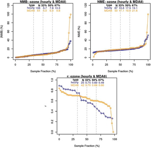
Figures S5 through S10 in the Supplemental Information show rank-ordered distributions for 1-hr and MDA8 ozone statistics separated according to pre-2012 publications, without Koo et al. (2015) and Yu et al. (2014), CMAQ/eastern United States/summer applications, rural monitors, cold season, and whether cutoffs were applied, as a way to show variability among these dimensions. Not all dimensions are shown on all plots because of insufficient numbers of data points from which to derive reliable distributions in such cases. In most cases we imposed a requirement for N ≥ 10, except in the case of cutoffs where results appear to be informative. Little NMB variability among these dimensions is exhibited for both 1-hr and MDA8 ozone, indicating rather consistent bias results across different groups of studies. The same is generally true for NME, except that unsigned error tends to be much larger for 1-hr ozone when no cutoffs are applied (i.e., when NME includes hours when observations approach zero). This result is not particularly surprising when considering that as the number of site-hours with low concentrations increase, the normalizing mean observation decreases and NME is skewed toward larger values (though not as extensively as MNE would be). Fewer dimensions were plotted for correlation coefficient due to the lack of data points; results for MDA8 show little difference whereas results for 1-hr ozone show a tendency for larger r achieved in pre-2012 studies. The reasons for this are not clear, though smaller ozone concentration ranges common in more recent years can degrade r values. Furthermore, we find that, as one would expect, including cutoffs in the calculation of r results in worse correlation because of fewer data points and because variability in only the upper range of ozone concentrations is considered. Therefore, we recommend that correlation coefficient be calculated for the entire range of paired prediction–observation pairs to yield a more robust and meaningful statistic.

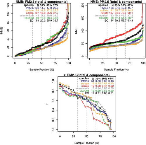
Figure 2 shows the combined rank-ordered distributions of NMB, NME, and r data points for total and speciated PM_2.5 from all studies cited in Tables 1 and 2. NMB and NME statistics exhibit much more variability than for ozone, especially for species historically difficult to simulate such as nitrate and carbon (organic and elemental). Over the 33–67th percentile interval, NMB ranges from 11 to 27% for total PM_2.5, sulfate, and ammonium, 20 to 33% for elemental carbon, 16 to 38% for nitrate, and 14 to 46% for organic carbon. NME ranges from 36 to 47% for PM_2.5, sulfate, and ammonium, 47 to 63% for carbon, and 65 to 90% for nitrate. Total PM_2.5 consistently exhibits smaller bias and error on par with sulfate and ammonium, which tend to be among the largest contributors to the PM_2.5 mass budgets at most locations throughout the United States. However, PM_2.5 bias also includes compensatory effects from other component species exhibiting much larger positive and negative biases. Correlation coefficients are consistently around 0.7 at the 33rd percentile regardless of PM species, while the 67th percentile values range from 0.6 for ammonium and organic carbon, to 0.5 for total PM_2.5 and elemental carbon, to 0.4 for sulfate, and 0.2 for nitrate.

Figure 2. Rank-ordered distributions of NMB, NME, and r statistics for total PM_2.5 and component species from all studies listed in Tables 1 and 2. Each panel shows (dashed gray line) and lists (text) the 33rd, 50th, and 67th percentile values and the total number of data points in each ranked distribution. EC refers to elemental carbon; OC/OM refers to organic carbon or total organic mass.

Figures S11 through S28 show additional rank-ordered distributions for total and speciated PM_2.5 separated into groups by pre-2012 publications, without Koo et al. (2015) and Yu et al. (2014), CMAQ/eastern United States/summer applications, rural monitors, and cold season. As for ozone, we imposed the same minimum number of data points (N ≥ 10) for these dimensions and cutoffs were not considered due to insufficient data points. NMB, NME, and r for total PM_2.5 all show little variation over these dimensions (Figures S11 through S13). Results for sulfate are also fairly consistent but with a bit more variability (Figures S14 through S16); slightly larger bias is evident for rural and CMAQ/eastern United States/summer applications, while slightly larger error occurs for the cold season group. Sulfate bias and error are notably smaller for pre-2012 studies, but the reasons for this are not clear. Similarly consistent results are also evident for the two groups plotted for ammonium (Figures S17 through S19). Not surprisingly, a larger degree of variability is noted for nitrate, particularly with the pre-2012, rural, and CMAQ/eastern United States/summer groups exhibiting far worse performance than the composite despite the pre-2012 group exhibiting slightly better correlation (Figures S20 through S22). As for organic carbon (Figures S23 through S25), NME exhibits little variability among groups while much more spread is noted for NMB, where the cold-season group has much larger bias (likely due to much lower observed organics in winter) and all other groups have much smaller bias than the composite. Elemental carbon exhibits similar variability as organic carbon with larger NMB and NME for the cold season, and smaller NME for the rural and pre-2012 groups (Figures S26 through S28). The larger variability for carbonaceous PM components among these groups may be related to different ways various studies have treated natural and event-oriented (fire) emission contributions.

Recommended metrics and benchmarks

On the basis of our analyses described above and illustrated in the Supplemental Information, Table 4 lists our recommended goals and criteria for NMB, NME, and r for 1-hr and MDA8 ozone and 24-hr total PM_2.5 and component species. We avoid listing correlation goals and criteria for nitrate, elemental and organic carbon because of large statistical uncertainty in determining their 33rd and 67th percentiles. Table 4 also notes past benchmarks for ozone (EPA, 1991) and PM (Boylan and Russell, 2006).

Table 4. Recommended benchmarks for photochemical model performance statistics: ozone, sulfate (SO₄), nitrate (NO₃), ammonium (NH₄), elemental carbon (EC) and organic carbon (OC).

	NMB		NME		r
Species	Goal	Criteria	Goal	Criteria	Goal	Criteria
1-hr or MDA8 Ozone	<±5%	<±15%	<15%	<25%	>0.75	>0.50
24-hr PM2.5, SO4, NH4	<±10%	<±30%	<35%	<50%	>0.70	>0.40
24-hr NO3	<±15%	<±65%	<65%	<115%	None	None
24-hr OC	<±15%	<±50%	<45%	<65%	None	None
24-hr EC	<±20%	<±40%	<50%	<75%	None	None

Note. We avoid listing correlation benchmarks for NO₃, EC, and OC because of large statistical uncertainty in determining their 33rd and 67th percentiles. “Goals” indicate statistical values that about a third of top performing past applications have met, and should be viewed as the best a model can be expected to achieve. “Criteria” indicate statistical values that about two thirds of past applications have met, and should be viewed as what a majority of models have achieved. The outlying one-third of past applications that exceed the criteria are considered poor performers for the particular metric and chemical species. See the text for additional information on the metrics and benchmarks. In addition:

1. We recommend a 40-ppb cutoff for 1-hr zone NMB and NME, but no cutoff r.

2. We recommend no cutoff for any statistics reported for MDA8 ozone.

3. Temporal scales for ozone statistics should not exceed 1 month; spatial scales should range from urban to ≤1000 km.

4. We recommend no cutoff for any statistics reported for 24-hr total and speciated PM.

5. Temporal scales for 24-hr total and speciated PM should not exceed 3 months (or 1 season); spatial scales should range from urban to ≤1000 km.

6. EPA (1991) benchmarks for 1-hr ozone: MNB < ±15%, MNE < 35%.

7. Boylan and Russell (2006) goals for 24-hr total and speciated PM: FB < ±30%, FE < 50%.

8. Boylan and Russell (2006) criteria for 24-hr total and speciated PM: FB < ±60%, FE < 75%.

Relative to past benchmarks for ozone and PM, the rank-ordered distributions shown in Figures 1 and 2 indicate that statistical performance has improved over the years, as past benchmarks are at the upper tails of the distributions in most cases. As a result, our recommended bias and error benchmarks are mostly stricter than previous benchmarks, particularly for ozone and generally for PM. Boylan and Russell (2006) recommended PM fractional bias and error criteria of 60% and 75%, respectively. A fractional value of 60% is equivalent to NM values ranging from 46% (underprediction) to 86% (overprediction), while a fractional value of 75% is equivalent to NM values ranging from 55% to 120%. Our recommended PM NMB criteria range from 30% to 65% and our PM NME criteria range from 50% to 115%, with nitrate at the upper end of both NMB and NME ranges. Our analysis of separate ranked distributions for various seasons, regions, and the few studies contributing a majority of data points (described in the preceding) indicates little sensitivity in ranked distributions for many metrics and species, with a few notable outliers. Therefore, our selection of goals and criteria is fairly robust against a few potentially influencing data sets. Of the 44 cases in which NMB, NME, and r statistics for ozone (both hourly and MDA8) were reported together in the studies listed in Tables 1 and 2, 23 cases (52%) achieved all three proposed criteria and 4 (9%) achieved all three goals. Of the 35 cases reporting all three statistics together for total PM_2.5, 14 cases (40%) achieved all three criteria and 1 case (3%) achieved all three goals.

One issue surrounding average-based statistical metrics is that they generally appear better with increasing number of data pairs due to larger influences from compensating effects, so calculating a single set of statistics over very large areas and/or long periods does not yield significant insight into performance. Therefore, NMB, NME, and r statistics should be calculated at appropriate space and time scales. Table 4 notes our recommended maximum scales. For both ozone and PM, we recommend calculating statistics over urban to regional scales, not to exceed about 1000 km. For ozone, we recommend calculating statistics over temporal scales of roughly 1 week (an episode), not to exceed 1 month. For PM we recommend statistics over temporal scales of 1 month, not to exceed 3 months (i.e., a single season), given the less frequent sampling schedule for PM components (typically every 3 or 6 days).

We do not recommend the use of cutoff values for most statistics, except for hourly ozone NMB and NME as a way to limit these statistics to daytime or ozone-forming conditions. Figure S7 shows a clear NME sensitivity to the removal of cutoffs in our rank-ordered distribution analysis, which is likely the result of poorer model performance over night. Models often lack skill in replicating low or zero ozone during stable or nocturnal NO_x-rich conditions. While not an indictment of chemical mechanisms per se, such problems are most often related to grid resolution and external inputs (e.g., inadequate characterization of shallow nocturnal boundary layers and mixing rates) that lead to poor characterization of emitted precursor concentrations. We suggest applying a cutoff value of 40 ppb for 1-hr ozone NMB and NME as a general demarcation between nocturnal ozone destruction and daytime ozone production regimes. While less than the 60-ppb cutoff currently recommended by EPA (2007, 2014), our recommendation remains in line with EPA’s reasoning to focus bias and error statistics on times of higher ozone, yet includes more daytime prediction–observation pairings than 60 ppb would afford, not just observations approaching the current standard. The choice of 40 ppb is not absolute and should consider the chemical climatology of the region being modeled. The issue of cutoffs in MPEs should be revisited in the future.

Additional recommendations for good practice

Although the MPE metrics presented in Table 4 give a general view of model performance, they are inadequate to fully inform modelers and stakeholders as to how well a PGM captures the pollutant dynamics that affect the specific end quantities and outcomes of interest being addressed in each type of application. Recognizing that PGMs are used to support various objectives, we recommend additional purposeful techniques for MPE.

Graphical plots are useful for evaluating models in conjunction with statistics. Specifically, time series (either as individual sites, or as means and variability over multiple sites), scatter diagrams (time-paired regression or time-unpaired rank-ordered comparisons), and cumulative distribution plots are particularly useful for understanding model performance and model behavior over entire ranges of concentrations. Foley et al. (2010) evaluate model bias and error for specific concentration ranges (or bins). Similar to scatter diagrams and regression analysis, the approach illustrates how the model is performing on different types of days or pollutant conditions that are relevant for specific applications. In addition, it is a good practice to generate spatial plots of bias and error for different portions of the modeling period (e.g., seasonally). Often referred to as “dot plots,” such maps present statistical results as color-coded markers at monitoring sites. These clearly demonstrate which monitors in the region are performing better or worse than others.

Thunis et al. (2011) describe the centered root mean square error (CRMSE), an alternative operational evaluation metric that relates correlation coefficient to standard deviations in predicted and observed variability. These relationships can be graphically depicted through the use of Taylor diagrams (Taylor, 2001). Solazzo and Galmarini (2016) present a spectral decomposition of model error over four different temporal scales ranging from intraday to several weeks, and further break out each scale-specific error into bias, variance, and unexplained components. As a hybrid between operation and diagnostic evaluation, such decomposition can reveal the temporal scales where the error is dominant and may give clearer indications on the processes contributing to error. These methods can provide additional powerful information on what drives model performance, and thus insight into model application weaknesses, so we recommend considering their use in future studies.

Most regulatory analyses focus on just a limited spectrum of the PGM results, for example, days with elevated pollutant levels. Given that regulations and the forms of air quality standards vary by country, the specific model results to be evaluated will be country and application specific, but they should be chosen to examine how well the PGM captures the pollutant dynamics relative to the regulatory outcomes of interest. The discussion that follows is specific to the United States, where PGMs are widely used in regulatory applications such as State Implementation Plans; Regulatory Impact Analyses; various transport, visibility, and deposition assessments; and to support the NAAQS review process (e.g., EPA, 2011b, 2011c, 2011d). PGM applications addressing ozone and PM NAAQS extract specific concentrations that align with the forms of the respective air quality standards (EPA, 2007, 2014). This includes the annual 4th-highest MDA8 ozone, annual 98th percentile 24-hr PM_2.5, and annual-average 24-hr PM_2.5. For ozone, EPA (2014) guidance recommends averaging the top 10 simulated seasonal MDA8 ozone values by monitoring site from both baseline and projection scenarios to develop a scaling factor (relative response factor, or RRF). The RRF is applied to each monitor’s 5-year average 4th highest MDA8 ozone to project measured conditions to the projection scenario, a practice that EPA adopted to address model–observation disagreements. The approach is similar for PM, though somewhat more complicated by the need to develop RRFs for individual PM species and the use of quarterly RRFs to project annual average PM_2.5.

For U.S. regulatory applications, we recommend extending the general MPE to focus bias and error calculations on the number of modeled days used in developing the RRFs for each species (ozone or PM components). Given that projections of air quality are conducted on a site-specific basis, site-specific performance should be evaluated, with particular emphasis on those locations that are of most importance in the analysis (e.g., locations that are currently and/or projected to exceed the applicable standard). We do not make recommendations for model performance benchmarks for individual monitors, recognizing that the importance of model performance at a specific site is application-specific. It is of interest to identify which location the model performs less well and to assess potential factors and the importance of the poorer performance in that area to the model application.

PGM applications can also include assessing ozone and PM transport contributions from specific sources, regions or categories to receptors in other regions. Typically, such applications require running the model using so-called “brute-force” methods (i.e., zeroing out emissions from one source at a time), source apportionment algorithms (Dunker et al., 2002), or sensitivity algorithms like adjoint (Menut et al., 2000) or decoupled-direct methods (Dunker, 1981; Hakami et al., 2003). For example, EPA (2011d) addressed interstate transport using source apportionment to calculate the individual contributions of emissions from every state in the eastern United States to air quality in other states. In that assessment, an upwind state’s contribution to a downwind state’s exceeding ozone monitor was considered significant if it contributed more than 1% of the ozone NAAQS over a set of exceedance or otherwise high ozone days projected in 2017.

Because of the regulatory implications resulting from being designated a significant contributor, it becomes critical to analyze model performance by evaluating bias and error at specific receptors and over the range of days included in the contribution assessment (as similarly described above). The statistical metrics recommended previously may not be adequate to characterize a model’s ability to report monitor-specific peak contributions accurately if those metrics are reported only for large regions or longer periods. If model performance is deemed inadequate at key receptors over the range of days included in the contribution assessment, it becomes critical to investigate the reasons for poor performance and to take measures to improve model performance before using the results for regulatory action.

We have not touched on the performance of meteorological models used to drive “off-line” or decoupled PGMs, as it is often implicitly assumed that if a PGM performs within certain benchmarks, the overall modeling system is performing adequately. However, for PGM applications related to source contributions, establishing adequate characterization of source-receptor transport patterns may be more critical than for other regulatory applications. Therefore, it becomes important to evaluate meteorological model performance in addition to the PGM. It is beyond the scope of this paper to recommend approaches for a general meteorological MPE, but one could use metrics previously established (e.g., Emery et al., 2001). Additionally, it is important to evaluate the specific transport routes for the subset of days when source–receptor contributions exceed certain thresholds—similar to our recommendations for the PGM application. Beyond simple wind speed/direction assessments for those days, it is critical to conduct trajectory analysis or “vector displacement” types of calculations that integrate wind speed and direction along the transport path to ensure that the transport patterns are consistent with those that actually occurred.

Conclusion

The growing use and importance of PGMs in a range of applications motivate the need to conduct more comprehensive performance evaluations that inform the user and affected community of model uncertainties and weaknesses as well as potential improvements. Further, such evaluations should be done in a consistent fashion such that results can be compared across applications, thereby providing context, and the ability to assess the extent to which model performance is or is not improving. Such evaluations can also serve to drive improvements in the modeling process as the major weaknesses are identified and addressed. In this paper we recommend a concise set of MPE metrics and associated benchmarks that should be evaluated for any PGM application.

Traditionally, three forms of normalized bias and error metrics have been used to characterize model performance: fractional, mean normalized (MN), and normalized mean (NM). While issues are identified with all three forms, NM-based statistics are deemed to have the best characteristics overall. Historically a cutoff value has been used when calculating ozone performance: Use of NM metrics obviates the need of a cutoff, or the sensitivity to its choice.

A literature review of historical PGM performance statistics developed by Simon et al. (2012), and extended in this study, was used to develop rank-ordered distributions of MPE metrics for NMB, NME and r. By evaluating those distributions, we developed pollutant-specific benchmarks for each of those metrics. Following ideas developed by Boylan and Russell (2006), we developed MPE benchmarks for goals and criteria (Table 4): the more restrictive goals represent about a third of most PGM applications over the past 10 years, while the less restrictive criteria represents about two-thirds, establishing historical context. By developing separate ranked distributions for various seasons, regions, and the few studies contributing a majority of data points, we found little sensitivity in ranked distributions for most (but not all) metrics or species. Therefore our selection of goals and criteria are fairly robust against a few potentially influencing data sets.

In selecting correlation coefficient (r) as one of our recommended MPE statistics, we sought a simple widely-used metric to characterize agreement between predicted and observed variability. However, the amount of agreement indicated by r depends on the number of prediction–observation pairs and this affects its reliability for comparing among different studies. Thus, it is equally important to report the confidence interval of r, which is used to quantify its statistical robustness.

We recommend applying a cutoff value of 40 ppb when calculating NMB and NME for 1-hr ozone, for several physical and regulatory reasons beyond the need for statistical stability, but not for correlation as it is best characterized over the entire concentration distribution. The choice of 40 ppb is not absolute and should consider the chemical climatology of the region being modeled. We recommend against the use of cutoffs for MDA8 ozone, total PM_2.5 and its components. Finally, MNB, MNE, and r should be calculated for prediction–observation pairs over time periods no longer than 1 month for ozone and 3 months for PM_2.5, and over spatial scales of less than ~1000 km. The mean of observed quantities and number of simulation–observation pairs used for the specific compounds being addressed should be reported.

Our recommendations include additional analyses, metrics, and graphics that should be developed in good practice to better characterize model performance, particularly for regulatory demonstrations (high-percentile vs. seasonal/annual average concentrations) and regional transport and source attribution. There will be a need to revisit periodically the MPE benchmarks and the issue of cutoffs as model performance changes, either due to improvements in input data sets and science treatments or perhaps as a result of changing air quality. In addition, as the community starts using and reporting on specific MPE metrics recommended for specific applications, information can be gathered to develop benchmarks for those metrics.

Acknowledgment

The authors thank Dr. Heather Simon, U.S. EPA, for providing the compilation of model performance data documented in Simon et al. (2012).

Funding

This work was supported by the Electric Power Research Institute.

Supplemental data

Supplemental data for this article can be accessed on the publisher’s website.

Additional information

Funding

This work was supported by the Electric Power Research Institute.

Notes on contributors

Christopher Emery

Christopher Emery is a senior manager at Ramboll Environ in Novato, CA.

Zhen Liu

Zhen Liu is a senior associate at Ramboll Environ in Novato, CA.

Armistead G. Russell

Armistead G. Russell is the Howard T. Tellepsen Chair and Regents’ Professor of Civil and Environmental Engineering at Georgia Institute of Technology in Atlanta, GA.

M. Talat Odman

M. Talat Odman is a principal research engineer in the School of Civil and Environmental Engineering at Georgia Institute of Technology in Atlanta, GA.

Greg Yarwood

Greg Yarwood is a principal at Ramboll Environ in Novato, CA.

Naresh Kumar

Naresh Kumar is a senior program manager at the Electric Power Research Institute in Palo Alto, CA.

References

- Baker, K., and P. Scheff. 2007. Photochemical model performance for PM2.5 sulfate, nitrate, ammonium, and precursor species SO2, HNO3, and NH3 at background monitor locations in the central and eastern United States. Atmos. Environ. 41:6185–95. doi:10.1016/j.atmosenv.2007.04.006
- Bessagnet, B., A. Hodzic, R. Vautard, M. Beekmann, S. Cheinet, C. Honoré, C. Liousse, and L. Rouil. 2004. Aerosol modeling with CHIMERE: Preliminary evaluation at the continental scale. Atmos. Environ. 38:2803–17. doi:10.1016/j.atmosenv.2004.02.034
- Boylan, J.W., and A.G. Russell. 2006. PM and light extinction model performance metrics, goals, and criteria for three-dimensional air quality models. Atmos. Environ. 40:4946–59. doi:10.1016/j.atmosenv.2005.09.087
- Brandt, J., J.H. Christensen, L.M. Frohn, C. Geels, K.M. Hansen, G.B. Hedegaard, M. Hvidberg, and C.A. Skjøth. 2007. THOR—An operational and integrated model system for air pollution forecasting and management from regional to local scale. Proceedings of the 2nd ACCENT Symposium, Urbino (Italy), July 23–27, 2007.
- Byun, D.W., S.T. Kim, and S.B. Kim. 2007. Evaluation of air quality models for the simulation of a high ozone episode in the Houston metropolitan area. Atmos. Environ. 41:837–53. doi:10.1016/j.atmosenv.2006.08.038
- Dennis, R., T. Fox, M. Fuentes, A. Gilliland, S. Hanna, C. Hogrefe, J. Irwin, S.T. Rao, R, Scheffe, K. Schere, D.A. Steyn, and A. Venkatram. 2010. A framework for evaluating regional-scale numerical photochemical modeling systems. J. Environ. Fluid Mech. 10:471–89. doi: 10.1007/s10652-009-9163-2.
- Downey, N., C. Emery, J. Jung, T. Sakulyanontvittaya, L. Hebert, D. Blewitt, and G.Yarwood. 2015. Emission reductions and urban ozone responses under more stringent US standards. Atmos. Environ. 101:209–16. doi: 10.1016/j.atmosenv.2014.11.018
- Dunker, A.M. 1981. Efficient calculation of sensitivity coefficients for complex atmospheric models. Atmos. Environ. (Part A) 15:1155–61. doi:10.1016/0004-6981(81)90305-X
- Dunker, A.M., G. Yarwood, J.P. Ortmann, and G.M. Wilson. 2002. Comparison of source apportionment and source sensitivity of ozone in a three-dimensional air quality model. Environ. Sci. Technol. 36:2953–64. doi:10.1021/es011418f
- Eder, B., D. Kang, R. Mathur, J. Pleim, S. Yu, T. Otte, and G. Pouliot. 2009. A performance evaluation of the National Air Quality Forecast Capability for the summer of 2007. Atmos. Environ. 43:2312–20. doi:10.1016/j.atmosenv.2009.01.033
- Emery, C., E. Tai, and G. Yarwood. 2001. Enhanced Meteorological Modeling and Performance Evaluation for Two Texas Ozone Episodes. Report to the Texas Natural Resources Conservation Commission, prepared by ENVIRON International Corp, Novato, CA. http://www.tceq.state.tx.us/assets/public/implementation/air/am/contracts/reports/mm/EnhancedMetModelingAndPerformanceEvaluation.pdf.
- Emery, C., J. Jung, N. Downey, J. Johnson, M. Jimenez, G. Yarwood, and R. Morris. 2012. Regional and global modeling estimates of policy relevant background ozone over the United States. Atmos. Environ. 47:206–217. doi:10.1016/j.atmosenv.2011.11.012
- Foley, K.M., S.J. Roselle, K.W. Appel, P.V. Bhave, J.E. Pleim, T.L. Otte, R. Mathur, G. Sarwar, J.O. Young, R.C. Gilliam, et al. 2010. Incremental testing of the Community Multiscale Air Quality (CMAQ) modeling system version 4.7. Geoscientific Model Dev. 3:205–26. doi:10.5194/gmd-3-205-2010
- Foley, K.M., C. Hogrefe, G. Pouliot, N. Possiel, S.J. Roselle, H. Simon, and B. Timin. 2015. Dynamic evaluation of CMAQ part I: Separating the effects of changing emissions and changing meteorology on ozone levels between 2002 and 2005 in the eastern US. Atmos. Environ. 103:247–55. doi:10.1016/j.atmosenv.2014.12.038
- Gaydos, T.M., R. Pinder, B. Koo, K.M. Fahey, G. Yarwood, and S.N. Pandis. 2007. Development and application of a three-dimensional aerosol chemical transport model, PMCAMx. Atmos. Environ. 41:2594–611. doi:10.1016/j.atmosenv.2006.11.034
- Grell, G.A., S. Emeis, W.R. Stockwell, T. Schoenemeyer, R. Forkel, J. Michalakes, R. Knoche, and W. Seidl. 2000. Application of a multiscale, coupled MM5/chemistry model to the complex terrain of the VOTALP valley campaign. Atmos. Environ. 34:1435–53. doi:10.1016/S1352-2310(99)00402-1
- Grell, G.A., S.E. Peckham, R. Schmitz, S.A. McKeen, G. Frost, W.C. Skamarock, and B. Eder. 2005. Fully coupled “online” chemistry within the WRF model. Atmos. Environ. 39:6957–75. doi:10.1016/j.atmosenv.2005.04.027
- Hakami, A., M.T. Odman, and A.G. Russell. 2003. High-order, direct sensitivity analysis of multidimensional air quality models. Environ. Sci. Technol. 37:2442–52. doi:10.1021/es020677h
- Harvard University. 2015. GEOS-Chem Online User’s Guide. Atmospheric Chemistry Modeling Group, School of Engineering and Applied Sciences, Harvard University, Cambridge, MA (http://acmg.seas.harvard.edu/geos/doc/man/index.html).
- Hogrefe, C., W. Hao, K. Civerolo, J.Y. Ku, G. Sistla, R.S. Gaza, L. Sedefian, K. Schere, A. Gilliland, A., and R. Mathur. 2007. Daily simulation of ozone and fine particulates over New York State: Findings and challenges. J. Appl. Meteorol. Climatol. 46:961–79. doi:10.1175/JAM2520.1
- Hogrefe, C., K.L. Civerolo, W. Hao, J.Y. Ku, E.E. Zalewsky, and G. Sistla. 2008. Rethinking the assessment of photochemical modeling systems in air quality planning applications. J. Air Waste Manage. Assoc. 58:1086–99. doi:10.3155/1047-3289.58.8.1086
- Hogrefe, C., W. Hao, E.E. Zalewsky, J.Y. Ku, B. Lynn, C. Rosenzweig, M.G. Schultz, S. Rast, M.J. Newchurch, L. Wang, P.L. Kinney, and G. Sistla. 2011. An analysis of long-term regional-scale ozone simulations over the northeastern United States: Variability and trends. Atmos. Chem. Phys. 11:567–82. doi:10.5194/acp-11-567-2011
- Hou, X., M.J. Strickland, and K.J. Liao. 2015. Contributions of regional air pollutant emissions to ozone and fine particulate matter-related mortalities in eastern U.S. urban areas. Environ. Res. 137:475–84. doi:10.1016/j.envres.2014.10.038
- Im, U., R. Bianconi, E. Solazzo, I. Kioutsioukis, A. Badia, A. Balzarini, R. Baro, R. Bellasio, D. Brunner, C. Chemel, G. Curci, et al. 2015. Evaluation of operational on-line-coupled regional air quality models over Europe and North America in the context of AQMEII Phase 2. Part I: Ozone. Atmos. Environ. 115:404–20. doi:10.1016/j.atmosenv.2014.08.072
- Jin, L., N.J. Brown, R.A. Harley, J.W. Bao, S.A. Michelson, and J.M. Wilczak. 2010. Seasonal versus episodic performance evaluation for an Eulerian photochemical air quality model. J. Geophys. Res. Atmos. 115:D09302. doi:10.1029/2009JD012680
- Kang, D., R. Mathur, and S.T. Rao. 2010. Real-time bias-adjusted O3 and PM2.5 air quality index forecasts and their performance evaluations over the continental United States. Atmos. Environ. 44:2203–12. doi:10.1016/j.atmosenv.2010.03.017
- Karamchandani, P., K. Vijayaraghavan, S.Y. Chen, C. Seigneur, and E.S. Edgerton, 2006. Plume-in-grid modeling for particulate matter. Atmos. Environ. 40:7280–97. doi:10.1016/j.atmosenv.2006.06.033
- Kim, Y., J.S. Fu, and T.L Miller. 2010. Improving ozone modeling in complex terrain at a fine grid resolution—Part II: influence of schemes in MM5 on daily maximum 8-h ozone concentrations and RRFs (Relative Reduction Factors) for SIPs in the non-attainment areas. Atmos. Environ. 44:2116–24. doi:10.1016/j.atmosenv.2010.02.038
- Koo, B., N. Kumar, E. Knipping, U. Nopmongcol, T. Sakulyanontvittaya, M.T. Odman, A.G. Russell, and G. Yarwood. 2015. Chemical transport model consistency in simulating regulatory outcomes and the relationship to model performance. Atmos. Environ. 116:159–71. doi:10.1016/j.atmosenv.2015.06.036
- Lee, D., D.W. Byun, H. Kim, F. Ngan, S.Kim, C. Lee, and C. Cho. 2011. Improved CMAQ predictions of particulate matter utilizing the satellite-derived aerosol optical depth. Atmos. Environ. 45:3730–41. doi:10.1016/j.atmosenv.2011.04.018
- Liao, K.-J., X. Hou, and D. R. Baker. 2014. Impacts of interstate transport of pollutants on high ozone events over the Mid-Atlantic United States. Atmos. Environ. 84:100–12. doi:10.1016/j.atmosenv.2013.10.062
- Liu, X.-H., Y. Zhang, K.M. Olsen, W.-X, Wang, B.A. Do, and G.M. Bridgers. 2010. Responses of future air quality to emission controls over North Carolina, Part I: Model evaluation for current-year simulations. Atmos. Environ. 44:2443–56. doi:10.1016/j.atmosenv.2010.04.002
- Makar, P.A., W. Gong, C. Mooney, J. Zhang, D. Davignon, M. Samaali, M.D. Moran, H. He, D.W. Tarasick, D. Sills, and J. Chen. 2010. Dynamic adjustment of climatological ozone boundary conditions for air-quality forecasts. Atmos. Chem. Phys. 10:8997–9015. doi:10.5194/acp-10-8997-2010
- Makar, P.A., W. Gong, C. Hogrefe, Y. Zhang, G. Curci, R. Zabkar, J. Milbrandt, U. Im, S. Galmarini, A. Balzarini, et al. 2015. Feedbacks between air pollution and weather, Part 1: Effects on chemistry. Atmos. Environ. 115:499–526. doi:10.1016/j.atmosenv.2014.10.021
- Marmur, A., W. Liu, Y. Wang, A.G. Russell, and E.S. Edgerton. 2009. Evaluation of model simulated atmospheric constituents with observations in the factor projected space: CMAQ simulations of SEARCH measurements. Atmos. Environ. 43:1839–49. doi:10.1016/j.atmosenv.2008.12.027
- Menut, L., R. Vautard, M. Beekmann, and C. Honore. 2000. Sensitivity of photochemical pollution using the adjoint of a simplified chemistry-transport model. J. Geophys. Res. Atmos. 105:15379–402. doi:10.1029/1999JD900953
- National Research Council. 2007. Models in Environmental Regulatory Decision Making. Washington, DC: National Research Council of the National Academies. doi:10.17226/11972.
- Odman, T., and Z. Adelman. 2014. Emissions and Air Quality Modeling for SEMAP. Final Report to Southeastern States Air Resource Managers, Inc., December 31, 2014, Georgia Tech, http://semap.ce.gatech.edu/sites/default/files/files/SEMAP-Revised-Final-Report_Final.pdf.
- Pun, B.K., C. Seigneur, K. Vijayaraghavan, S.Y. Wu, S.Y. Chen, E.M. Knipping, and N. Kumar. 2006. Modeling regional haze in the BRAVO study using CMAQMADRID: 1. Model evaluation. J. Geophys. Res. Atmos. 111:D06302. doi:10.1029/2004JD005608
- Queen, A., and Y. Zhang. 2008. Examining the sensitivity of MM5-CMAQ predictions to explicit microphysics schemes and horizontal grid resolutions, Part II—PM concentrations and wet deposition predictions. Atmos. Environ. 42:3856–68. doi:10.1016/j.atmosenv.2007.12.066
- Ramboll Environ. 2016. User’s Guide: Comprehensive Air quality Model with extensions, Version 6.30. Ramboll Environ, Novato, CA (www.camx.com).
- Rodriguez, M.A., M.G. Barna, K.A. Gebhart, J.L. Hand, Z.E. Adelman, B.A. Schichtel, J.L. Collett, Jr., and W.C. Malm. 2011. Modeling the fate of atmospheric reduced nitrogen during the Rocky Mountain Atmospheric Nitrogen and Sulfur Study (RoMANS): Performance evaluation and diagnosis using integrated processes rate analysis. Atmos. Environ. 45:223–34. doi:10.1016/j.atmosenv.2010.09.011
- Sakulyanontvittaya, T., A. Guenther, D. Helmig, J. Milford, and C. Wiedinmyer. 2008. Secondary organic aerosol from sesquiterpene and monoterpene emissions in the United States. Environ. Sci. Technol. 42:8784–90. doi:10.1021/es800817r
- Simon, H., K.R. Baker, and S., Phillips. 2012. Compilation and interpretation of photochemical model performance statistics published between 2006 and 2012. Atmos. Environ. 61:124–39. doi:10.1016/j.atmosenv.2012.07.012
- Smyth, S.C., W.M. Jiang, D.Z. Yin, H. Roth, and T. Giroux. 2006. Evaluation of CMAQ O3 and PM2.5 performance using Pacific 2001 measurement data. Atmos. Environ. 40:2735–49. doi:10.1016/j.atmosenv.2005.10.068
- Smyth, S.C., W. Jiang, H. Roth, M.D. Moran, P.A. Makar, F. Yang, V.S. Bouchet, and H. Landry. 2009. A comparative performance evaluation of the AURAMS and CMAQ air-quality modelling systems. Atmos. Environ. 43:1059–70. doi:10.1016/j.atmosenv.2008.11.027
- Solazzo, E., R. Bianconi, G. Pirovano, V. Matthias, R. Vautard, K.W. Appel, B. Bessagnet, J. Brandt, J.H. Christensen, C. Chemel, et al. 2012. Operational model evaluation for particulate matter in Europe and North America in the context of AQMEII. Atmos. Environ. 53:75–92. doi:10.1016/j.atmosenv.2012.02.045
- Solazzo, E. and S. Galmarini. 2016. Error apportionment for atmospheric chemistry-transport models – A new approach to model evaluation. Atmos. Chem. Phys. 16:6263–6283 doi:10.5194/acp-16-6263-2016.
- Spak, S.N., and T. Holloway. 2009. Seasonality of speciated aerosol transport over the Great Lakes region. J. Geophys. Res. Atmos. 114:D08302. doi:10.1029/2008JD010598
- Stroud, C.A., P.A. Makar, M.D. Moran, W. Gong, S. Gong, J. Zhang, K. Hayden, C. Mihele, J.R. Brook, J.P.D. Abbatt, and J.G. Slowik. 2011. Impact of model grid spacing on regional- and urban- scale air quality predictions of organic aerosol. Atmos. Chem. Phys. 11:3107–18. doi:10.5194/acp-11-3107-2011
- Tang, W., D.S. Cohan, G.A. Morris, D.W. Byun, and W.T. Luke. 2011. Influence of vertical mixing uncertainties on ozone simulation in CMAQ. Atmos. Environ. 45:2898–909. doi:10.1016/j.atmosenv.2011.01.057
- Taylor, K.E. 2001. Summarizing multiple aspects of model performance in a single diagram. J. Geophys. Res. 106:7183–92. doi:10.1029/2000JD900719
- Tesche, T.W. 1988. Accuracy of ozone air-quality models. J. Environ. Eng. ASCE 114:739–52. doi:10.1061/(ASCE)0733-9372(1988)114:4(739)
- Thunis, P., E. Georgieva, and S. Galmarini. 2011. A procedure for air quality models benchmarking. Prepared by the Joint Research Centre, Ispra, Italy ( 16 February 2011). http://fairmode.jrc.ec.europa.eu/document/fairmode/WG1/WG2_SG4_benchmarking_V2.pdf
- U.S. EPA. 1990. User’s Guide for the Urban Airshed Model, Volume I: User’s Manual for UAM (CB-IV). U.S. Environmental Protection Agency, Research Triangle Park, NC (EPA-450/4-90-007A).
- U.S. EPA. 1991. Guideline for Regulatory Applications of the Urban Airshed Model. U.S. Environmental Protection Agency, Research Triangle Park, NC (EPA-450/4-91-013).
- U.S. EPA. 2007. Guidance on the Use of Models and Other Analyses for Demonstrating Attainment of Air Quality Goals for Ozone, PM2.5, and Regional Haze. U.S. Environmental Protection Agency, Research Triangle Park, NC (EPA-454/B-07-002).
- U.S. EPA. 2011a. Policy Assessment for the Review of the Secondary National Ambient Air Quality Standards for Oxides of Nitrogen and Oxides of Sulfur. U.S. Environmental Protection Agency, Research Triangle Park, NC ( EPA-452/R-11-005a, February).
- U.S. EPA. 2011b. The Benefits and Costs of the Clean Air Act from 1990 to 2020. U.S. Environmental Protection Agency, Washington, DC (March).
- U.S. EPA. 2011c. Policy Assessment for the Review of the Particulate Matter National Ambient Air Quality Standards. U.S. Environmental Protection Agency, Research Triangle Park, NC ( EPA 452/R-11-003, April).
- U.S. EPA. 2011d. Air Quality Modeling, Final Rule Technical Support Document. US Environmental Protection Agency, Research Triangle Park, NC (June).
- U.S. EPA. 2014. Draft Modeling Guidance for Demonstrating Attainment of Air Quality Goals for Ozone, PM2.5, and Regional Haze. U.S. Environmental Protection Agency, Research Triangle Park, NC ( December).
- Willmott, C.J. 1982. Some comments on the evaluation of model performance. Bull. Am. Meteorol. Soc. 63:1309–13. doi:10.1175/1520-0477(1982)063<1309:SCOTEO>2.0.CO;2
- Wong, D.C., J. Pleim, R. Mathur, F. Binkowski, T. Otte, R. Gilliam, G. Pouliot, A. Xiu, J.O. Young, and D. Kang. 2012. WRF-CMAQ two-way coupled system with aerosol feedback: software development and preliminary results. Geoscientific Model Dev. 5:299–312. doi:10.5194/gmd-5-299-2012.
- Wu, S.-Y., S. Krishnan, and Y. Zhang, V. Aneja. 2008. Modeling atmospheric transport and fate of ammonia in North Carolina—Part I: Evaluation of meteorological and chemical predictions. Atmos. Environ. 42:3419–36. doi:10.1016/j.atmosenv.2007.04.031
- Yu, S., R. Mathur, D. Kang, K. Schere, B. Eder, and J. Pleim. 2006. Performance and diagnostic evaluation of ozone predictions by the Eta-community multiscale air quality forecast system during the 2002 New England Air Quality Study. J. Air Waste Manage. Assoc. 56:1459–71. doi:10.1080/10473289.2006.10464554
- Yu, S., R. Mathur, K. Schere, D. Kang, J. Pleim, and T.L. Otte. 2007. A detailed evaluation of the Eta-CMAQ forecast model performance for O3, its related precursors, and meteorological parameters during the 2004 ICARTT study. J. Geophys. Res. Atmos. 112:D12s14. doi:10.1029/2006JD007715
- Yu, S., R. Mathur, J. Pleim, D. Wong, R. Gilliam, K. Alapaty, C. Zhao, and X. Liu. 2014. Aerosol indirect effect on the grid-scale clouds in the two-way coupled WRF–CMAQ: Model description, development, evaluation and regional analysis. Atmos. Chem. Phys. 14:11247–85. doi:10.5194/acp-14-11247-2014. doi:10.5194/acp-14-11247-2014
- Zhang, L.M., M.D. Moran, P.A. Makar, J.R. Brook, and S.L. Gong. 2002. Modelling gaseous dry deposition in AURAMS: A unified regional air-quality modelling system. Atmos. Environ. 36:537–60. doi:10.1016/S1352-2310(01)00447-2
- Zhang, Y., P. Liu, A. Queen, C. Misenis, B. Pun, C. Seigneur, and S.-Y. Wu. 2006. A comprehensive performance evaluation of MM5-CMAQ for the Summer 1999 Southern Oxidants Study episode—Part II: Gas and aerosol predictions. Atmos. Environ. 40:4839–55. doi:10.1016/j.atmosenv.2005.12.048
- Zhang, Y., J.-P. Huang, D.K. Henze, and J.H. Seinfeld. 2007. Role of isoprene in secondary organic aerosol formation on a regional scale. J. Geophys. Res. Atmos. 112:D20207. doi:10.1029/2007JD008675
- Zhang, Y., Y. Pan, K. Wang, J.D. Fast, and G.A. Grell. 2010. WRF/Chem-MADRID: Incorporation of an aerosol module into WRF/Chem and its initial application to the TexAQS2000 episode. J. Geophys. Res. Atmos. 115:D18202. doi:10.1029/2009JD013443