Development of the crop residue and rangeland burning in the 2014 National Emissions Inventory using information from multiple sources

ABSTRACT

Biomass burning has been identified as an important contributor to the degradation of air quality because of its impact on ozone and particulate matter. One component of the biomass burning inventory, crop residue burning, has been poorly characterized in the National Emissions Inventory (NEI). In the 2011 NEI, wildland fires, prescribed fires, and crop residue burning collectively were the largest source of PM_2.5. This paper summarizes our 2014 NEI method to estimate crop residue burning emissions and grass/pasture burning emissions using remote sensing data and field information and literature-based, crop-specific emission factors. We focus on both the postharvest and pre-harvest burning that takes place with bluegrass, corn, cotton, rice, soybeans, sugarcane and wheat. Estimates for 2014 indicate that over the continental United States (CONUS), crop residue burning excluding all areas identified as Pasture/Grass, Grassland Herbaceous, and Pasture/Hay occurred over approximately 1.5 million acres of land and produced 19,600 short tons of PM_2.5. For areas identified as Pasture/Grass, Grassland Herbaceous, and Pasture/Hay, biomass burning emissions occurred over approximately 1.6 million acres of land and produced 30,000 short tons of PM_2.5. This estimate compares with the 2011 NEI and 2008 NEI as follows: 2008: 49,650 short tons and 2011: 141,180 short tons. Note that in the previous two NEIs rangeland burning was not well defined and so the comparison is not exact. The remote sensing data also provided verification of our existing diurnal profile for crop residue burning emissions used in chemical transport modeling. In addition, the entire database used to estimate this sector of emissions is available on EPA’s Clearinghouse for Inventories and Emission Factors (CHIEF, http://www3.epa.gov/ttn/chief/index.html).Implications: Estimates of crop residue burning and rangeland burning emissions can be improved by using satellite detections. Local information is helpful in distinguishing crop residue and rangeland burning from all other types of fires.

Introduction

Biomass burning is one of the primary causes of elevated airborne particulate matter (PM), ozone precursors, and regional haze (Akimoto, 2003; Anderson et al., 2016b). PM is one of six pollutants for which the U.S. Environmental Protection Agency (EPA) has set National Ambient Air Quality Standards (NAAQS). PM_2.5 describes particles found in the air, including dust, dirt, soot, smoke, and liquid droplets, with a mean diameter of 2.5 microns or less. Biomass burning is an important source of primary PM_2.5, and precursor emissions that can form secondary PM_2.5. PM_2.5 has been linked to a series of significant health problems, including aggravated asthma, increases in respiratory symptoms such as coughing and difficult or painful breathing, chronic bronchitis, decreased lung function, and premature death (Bruenkreef and Holgate, 2002). The EPA has estimated that there were 23 million living in PM_2.5 nonattainment areas (using the 2012 standard) based on the 2010 census data (EPA, 2016b). Reducing emissions of PM is a crucial component of the EPA’s strategy for cleaner air and improved visibility.

The National Emissions Inventory (NEI) is a comprehensive and detailed estimate of air emissions of both criteria (CAPs) and hazardous (HAPs) air pollutants from all air emission sources. The NEI is prepared every 3 yr by the EPA on the basis of primarily emission estimates and emission model inputs provided by state, local, and tribal air agencies for sources in their jurisdictions and supplemented by data developed by the EPA. Emission inventories are the basis for trends analysis, regional- and local-scale air quality modeling, regulatory impact assessments, and human exposure modeling.

Many efforts have been made to improve wildland fire and prescribed fire emissions over last several NEI cycles since 2002. In 2002, the wildland fire and prescribed fire emission inventory was developed with extensive funding from regional planning organizations and the EPA (Pace and Pouliot, 2007). For the 2005 NEI, the wildfire and prescribed emission inventories were developed using SMARTFIRE version 1 (Raffuse et al., 2009). For the 2008 and 2011 NEIs, the wildfire and prescribed emission inventories were developed using SMARTFIRE version 2 (SF2). SMARTFIRE version 1 and version 2 are compared and described in Larkin et al. (2010). However, agricultural burning emission estimates are still somewhat deficient. In 2002, only 23 states reported emissions from this source (Pouliot et al., 2008), and in 2005, this source was not even updated in the NEI.

In the 2008 NEI (EPA, 2012), crop residue emission estimates have been developed using satellite detects occurring over land types classified as “agricultural” with a constant national default field size. A description of the 2008 NEI method for agricultural burning can be found in Supplemental Material. In the 2011 NEI, the method described in McCarty et al. (2009) and McCarty (2011) was employed to estimate the emissions from this sector, with the exception that states were allowed to submit their own estimates (EPA, 2016a). However, this produced significant variability between states that submitted their own data and states that did not because of different methodologies used to estimate emission factors and area burned.

Therefore, the goal of this work is to develop a simple and efficient method to estimate emissions from crop residue burning that can be easily applied across multiple years over the Contiguous United States (CONUS) at minimal cost. The approach being developed improves on previous estimates (McCarty et al., 2009; McCarty, 2011) as follows: (1) multiple satellite detections are used to locate fires using an operational product; (2) field size estimates are based on field work studies in multiple states (rather than a one-size-fits-all approach); and (3) this method allows for annual changes in crop land use. We will show CONUS emission estimates from crop residue burning for 2014 using a consistent methodology. This method is an modification to the method described in Pouliot et al. (2012) and is as follows: (1) additional processing of the Hazard Mapping System (HMS) data to remove two types of duplicates; (2) use of United States Department of Agriculture (USDA) National Agricultural Statistics Service Information (NASS) Cropland Data Layer (CDL) (USDA, 2015a) information to separate grass/pasture lands, which include pasture/grass, grassland herbaceous, and pasture/hay lands, from all other agricultural burning and (3) to identify the crop type removal of agricultural fires from the HMS (http://www.ospo.noaa.gov/Products/land/hms.html; Ruminski et al., 2006; Ruminski and Hanna, 2010) data set before the application of the SF2 system for wildfires and prescribed fires to eliminate double counting in the NEI; and (4) use of state information to further identify fires as crop residue burning rather than another type of fire. We compare the method used in this paper with Pouliot et al. (2012) because both methods are similar. The significant differences have been noted above, and the method described in this paper is more practical to implement. Our approach described in this paper complements the method used to estimate emissions from wildfires and prescribed fires because we use crop-level land use information to identify crop residue fires and grassland (rangeland) fires. The remaining fire detections are used in SF2 to estimate emissions in forested areas where fuel loadings are available from the U.S. Forest Service. The entire set of activity data, emission factors, and ancillary data is available on EPA’s Clearinghouse for Inventories and Emissions Factors (CHIEF) website (EPA, 2015).

Methods

Inputs used to create inventory

The HMS satellite product is an operational satellite product showing hot spots and smoke plumes indicative of fire locations. It is a blended product using algorithms for the Geostationary Operational Environmental Satellite (GOES) Imager, the Polar Operational Environmental Satellite (POES) Advanced Very High Resolution Radiometer (AVHRR), Moderate Resolution Imaging Spectroradiometer (MODIS), and more recently the Visible Infrared Imaging Radiometer Suite (VIIRS). A quality control procedure is performed by an analyst on the automated fire detections. Significant smoke plumes that are detected by the satellites are outlined by the analyst. This product is created and updated as needed operationally between the hours of 1 p.m. and 11 p.m. Eastern Time and released as a preliminary product. After 11 p.m., the analysis is fine-tuned (i.e., only minor changes are made) and a final product is released. The final fine-tuned analysis product was used for this study. These satellite detections are provided at 0.001° latitude or longitude, but they are derived from active fire satellite products ranging in spatial accuracy from 375 m to 4 km. Each fire detection has a spatial accuracy that is a function of the type of satellite instrument used in the detection. This means that the exact location of the fires is not accurate and could lead to incorrect identification.

To identify the crop type and to distinguish agricultural fires from all other fires in the HMS product, the USDA Cropland Data Layer (CDL) (USDA, 2015a) was employed. This data set is produced annually by the USDA National Agricultural Statistics Service and provides high-resolution (30 m) detailed crop information to accurately identify crop types for agricultural fires. According the USDA, the pasture- and grass-related land cover categories have traditionally had very low classification accuracy in the CDL (USDA, 2015b). Moderate spatial and spectral resolution satellite imagery is not ideal for separating grassy land use types, such as urban open space versus pasture for grazing versus Conservation Reserve Program (CRP) grass. To further complicate the matter, the pasture- and grass-related categories were not always classified consistently from state to state or year to year (USDA, 2015b). In an effort to eliminate user confusion and category inconsistencies, the 1997–2013 CDLs were recoded and re-released in January 2014 to better represent pasture- and grass-related categories (USDA, 2015b). A new category, named Grass/Pasture (code 176), collapses the following historical CDL categories: Pasture/Grass (code 62), Grassland Herbaceous (code 171), and Pasture/Hay (code 181). This new code (176) has been used to create a single grass/pasture emission source category separate from all other crop types.

Based on field reconnaissance of McCarty (2013, personal communication), a “typical” field size was assumed for each burn location, which varied by region of the country between 40 and 80 acres. The assumed field sizes can be found on the CHIEF website at http://www.epa.gov/sites/production/files/2015-06/draft_2014_ag_grasspasture_emissions_nei_may62015.xlsx. Emission Factors for carbon monoxide (CO), nitrogen oxides (NO_x), sulfur dioxide (SO₂), PM_2.5, and PM₁₀ were based on table 1 from McCarty (2011). The emission factors in McCarty (2011) were based on mean values from all available literature at the time. Emission factors for ammonia (NH₃) were derived from the 2002 NEI crop residue emission estimates using the ratio of NH₃/NO_x and the NO_x emission factor in table 1 from McCarty (2011). Note that in the 2002 NEI, this sector was estimated only with state-submitted data. We did not use NH₃ emission factors from the 2008 NEI because in these inventories, only one emission factor across all crop types was employed. In the 2011 NEI, NH₃ was not estimated for this sector except for those states (four in the CONUS) that submitted this information, and in these cases, the NH₃ factor was the same across all crop types. AP-42 emission factor ratios for volatile organic compound (VOC)/CO and the CO emission factors from table 1 in McCarty (2011) were used to estimate VOC emission factors. Table 1 shows the HAPs for which emissions were estimated.

Table 1. Emission factors, fuel loading, and combustion completeness for criteria air pollutants.

Crop type	Fuel loading (tons/acre)	Combustion completeness	CO (lbs/ton)	NOx (lbs/ton)	SO2 (lbs/ton)	PM2.5 (lbs/ton)	PM10 (lbs/ton)	VOC (lbs/ton)	NH3 (lbs/ton)
Corn	4.20^a	0.75^a	106.10^a	4.60^a	2.38^a	9.94^a	21.36^a	6.60^c	19.32^b
Wheat	1.90^a	0.85^a	110.28^a	4.75^a	0.88^a	8.07^a	14.10^a	7.60^c	33.73^b
Soybean	2.50^a	0.75^a	127.70^a	6.33^a	3.13^a	12.38^a	17.73^a	11.97^c	44.94^b
Cotton	2.18^a	0.65^a	146.12^a	6.89^a	3.13^a	12.38^a	17.73^a	11.97^c	48.92^b
Fallow	2.18^a	0.75^a	127.79^a	5.60^a	2.34^a	12.31^a	17.00^a	11.97^c	16.24^b
Rice	3.00^a	0.75^a	105.27^a	6.23^a	2.77^a	4.72^a	6.61^a	5.00^c	26.17^b
Sugarcane	4.75^a	0.65^a	116.95^a	6.06^a	3.32^a	8.69^a	9.83^a	9.00^c	43.03^b
Lentils	2.94^a	0.75^a	127.79^a	5.60^a	2.34^a	12.31^a	17.00^a	11.97^c	39.76^b
Other crops	1.90^a	0.85^a	182.11^a	4.31^a	0.80^a	23.23^a	31.64^a	10.70^c	12.52^b
Double crops
Winter wheat/Corn	3.05^d	0.80^d	108.19^d	4.68^d	1.63^d	9.00^d	17.73^d	7.10^d	26.53^d
Oats/Corn	3.19^d	0.75^d	116.95^d	5.10^d	2.36^d	11.13^d	19.18^d	8.45^d	21.41^d
Lettuce/Upland cotton	2.18^d	0.75^d	127.79^d	5.60^d	2.34^d	12.31^d	17.00^d	11.97^d	39.74^d
Durum wheat/Sorghum	2.04^d	0.80^d	119.04^d	5.17^d	1.61^d	10.19^d	15.55^d	6.35^d	36.74^d
Winter wheat/Sorghum	2.04^d	0.80^d	119.04^d	5.17^d	1.61^d	10.19^d	15.55^d	6.35^d	36.74^d
Barley/Corn	3.05^d	0.80^d	108.19^d	4.68^d	1.63^d	9.00^d	17.73^d	10.80^d	19.63^d
Winter wheat/Cotton	2.04^d	0.75^d	128.20^d	5.82^d	2.01^d	10.22^d	15.91^d	11.97^d	41.33^d
Soybeans/Cotton	2.34^d	0.7^d	136.91^d	6.61^d	3.13^d	12.38^d	17.73^d	11.97^d	46.94^d
Soybeans/Oats	2.34^d	0.75^d	127.75^d	5.96^d	2.74^d	12.35^d	17.36^d	11.97^d	42.35^d
Corn/Soybeans	3.35^d	0.75^d	116.90^d	5.46^d	2.76^d	11.16^d	19.55^d	11.97^d	22.94^d
Winter wheat/Soy	2.2^d	0.8^d	118.99^d	5.54^d	2.01^d	10.22^d	15.91^d	9.79^d	39.33^d
Lettuce/Durum wheat	2.04^d	0.8^d	119.04^d	5.17^d	1.61^d	10.19^d	15.55^d	9.79^d	36.74^d
Pasture_Grass	1.9^a	0.85^a	182.11^a	4.31^a	0.80^a	23.23^a	31.64^a	10.70^c	12.52^b

^aMcCarty (2011). Fuel loading and combustion completeness from table 1. Factors converted to lbs/ton.

^b2002 NEI NH₃/NO_X ratio.

^cVOC AP-42 factors ratio to CO factors from McCarty (2011).

^dAverage of two field crops.

Description of method

The HMS satellite detections were processed through five layers of filtering to find the locations of crop residue and rangeland burning. The first layer of filtering removed all detections outside the lower 48 states. The second layer of filtering removed the detections that were identified as wildland and prescribed fires because they occurred in a nonagricultural region. This identification was made by intersecting the USDA CDL with the remaining HMS detects to determine a crop type. Given that the satellite detections are at best known to 100 m and the CDL information is known to 30-m resolution, the process of intersecting these two data sets results in some uncertainty with respect to spatial accuracy of the fire locations. The third layer of filtering involved the use of snow cover estimates. Using the daily maximum snow cover data from a Weather Research and Forecasting (WRF) model (Skamarock et al., 2008) simulation for 2014, HMS satellite detections from GOES, MODIS, and AVHRR that were coincident with snow cover were deemed not to be crop residue burning but some other type of fire. The snow cover data in the WRF model are based on data assimilation of snow cover information and not on the precipitation field. The fourth layer of filtering was based on comments from specific states regarding specific crops. Corn and soybean detections for eight midwestern states (Iowa, Indiana, Illinois, Michigan, Missouri, Minnesota, Wisconsin, and Ohio) were deemed to be a non–crop residue burning fire. The reasoning is based on a communication from Iowa State University Extension and Outreach:

Burning corn and soybean fields is just NOT a practice that is used in Iowa or many other Midwest States as a way of preparing the fields for planting a subsequent crop. Yes, there are rare occasions where corn residue is burnt off a field but it would not even be 1% of the crop acres. An example would be if the residue washed and piled up in an area it may be burnt to allow tillage, planting and other practices to occur. Another rare occasion is when accidental field fires occur during harvesting of the corn crop. But again this would be less than 1% of the crop acres.

The full text of the analysis from the state of Iowa is included in Supplemental Material as Exhibit 1. Communication from the state of Indiana was similar to that of Iowa with respect to corn and soybeans, and so we make the same assumption (as in Iowa) about corn and soybeans in these states. The other six midwestern states (Illinois, Michigan, Missouri, Minnesota, Wisconsin, and Ohio) were included because of their proximity to the Indiana and Iowa so that the method would be consistent at a regional scale. These fires that are not being identified as crop residue burning or rangeland burning are being classified as accidental rather than intentional burning. Accidental fires are classified as wildfires regardless of the landscape on which they occur. These fire detections are included in the wildfire and prescribed fire emission inventory via the SMARTFIRE reconciliation process. Also as part of the fourth layer of filtering, if localized state information identified a fire as being accidental but in the vicinity of agricultural land, we deemed these fires not to be crop residue burning but in the wildfire category. This was the case for the state of Delaware. The fifth level of filtering was the process of removing duplicates. The remaining HMS satellite detections were checked for two types of duplicates. If a GOES detection was within 2 km and within an hour of another detection, the detection was deemed to be a duplicate and removed. Identical latitude and longitude detections to 3 decimal places on the same day across all satellites were also deemed to be duplicates and they were removed. For the first type of duplicate, approximately 1% of the total detections identified as agricultural were found to be duplicates. For the second type of duplicate, approximately 8% of the total detections identified as agricultural were found to be duplicates. Table 3 shows the number of HMS detections after each level of filtering. We note that of the detections that were in agricultural areas (i.e., not outside of the domain or identified as wildland/prescribed), 11% were in snow-covered areas, 6% were removed based on state data, 8% were duplicates, and 75% were retained for emission estimates.

Table 2. Emission factors for hazardous air pollutants.

HAP	Emission factor (lbs/ton)
1,3-Butadiene	0.354
Acetaldehyde	1.444
Anthracene	0.004
Benz[a]anthracene	0.004
Benzene	0.713
Benzo[a]pyrene	0.001
Benzo[e]pyrene	0.002
Benzo[g,h,i]perylene	0.003
Benzo[k]fluoranthene	0.002
Chrysene	0.004
Fluoranthene	0.008
Formaldehyde	3.370
Indeno[1,2,3-c,d]pyrene	0.002
Perylene	0.001
Phenanthrene	0.010
Pyrene	0.007
Toluene	0.470

Table 3. Count of HMS satellite detections by filtering level.

Filter level	Description	Count of HMS detections	% Agriculture/rangeland	Comments
1	Detections outside of lower 48 states	196,875		Included for SF2 processing
2	Detections that were not agricultural	108,203		Included for SF2 processing
3	Detections in snow-covered areas	6,701	11%	Included for SF2 processing
4	Detections removed from Iowa	944	1%	Included for SF2 processing
4	Detections removed from other midwestern states	2,911	5%	Included for SF2 processing
4	Detections Removed from Delaware	15	0%	Included for SF2 processing
5	Detections that were duplicates from GOES	336	1%	Not used
5	Detections that were duplicates across satellites	4,907	8%	Not used
6	Detections used for emission estimates	47,729	75%	Used in this study for emission estimates

Using the CAP and HAP emission factors in Tables 1 and 2, and the assumed region-specific field size, daily emissions were estimated for each fire detection. Emissions for the Grass/Pasture category were mapped to a single source classification code (SCC 2801500170) for use in the NEI. Emissions for all the remaining CDL categories were mapped to a set of source classification codes. Theses codes and the mapping are available at the CHIEF website (http://www.epa.gov/air-emissions-inventories/2014-national-emissions-inventory-nei-information).

Results and discussion

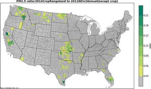
Table 4 summarizes state-level estimates of crop residue burning by acres burned and PM_2.5 emissions for 2014. These estimates were derived used the method described above. The top two states for crop residue burning (PM_2.5 emissions [tons/yr] and acres) were California and Kansas. The top two states for grass/pasture burns were Kansas and Oklahoma. For grasslands, we would expect these two states to have the largest acres burned because of the annual prescribed burning of the Flint Hills Grasslands and the large geographical extent of these regions. The grass/pasture burns are also known as rangeland burning, based on the definition of the grass/pasture land use in the Cropland Data Layer. Figure 1 provides a spatial map of the annual emissions by county for 2014 using this method for both crop residue and rangeland burning. We note that crop residue and rangeland burning are not widespread but occur in a few specific regions of the country. For context, Figure 2 shows the ratio of the 2014 emission estimates from this study to the 2011 NEIv2 emissions from all other sources excluding crop residue burning (the full 2014 NEI is not available). Figure 2 shows that there are a few counties in the CONUS where on an annual basis, crop residue and rangeland burning contribute up to 33% of the total PM_2.5 emissions for that county. However, for the majority of the counties, crop residue and rangeland burning contribute less than 3%.

Table 4. Acres burned and PM_2.5 emission estimates for 2014.

State	2014 Crop acres	2014 Crop PM2.5 (short tons/yr)	2014 Grass/pasture acres	2014 Grass/pasture PM2.5 (short tons/yr)
Alabama	21,000	307	32,240	605
Arizona	8,240	118	2,800	53
Arkansas	137,160	1,371	28,400	533
California	202,560	2,854	51,240	961
Colorado	4,240	63	3,840	72
Florida	147,540	2,142	79,440	1,490
Georgia	100,240	1,351	39,360	738
Idaho	50,880	650	35,400	664
Illinois	1,680	18	7,980	150
Indiana	660	7	3,480	65
Iowa	3,660	69	14,940	280
Kansas	180,720	2,207	461,600	8,655
Kentucky	8,000	110	7,760	146
Louisiana	87,920	1,052	20,000	375
Maryland	800	10	160	3
Massachusetts	80	2	40	1
Michigan	640	11	480	9
Minnesota	17,280	220	4,200	79
Mississippi	45,600	537	21,200	398
Missouri	31,980	327	71,880	1,348
Montana	32,760	428	32,640	612
Nebraska	29,820	419	25,200	473
Nevada	360	5	520	10
New Jersey	160	3	120	2
New Mexico	1,120	17	7,120	134
New York	600	10	320	6
North Carolina	32,000	406	8,200	154
North Dakota	117,480	1,402	29,700	557
Ohio	400	5	1,320	25
Oklahoma	49,440	506	299,600	5,618
Oregon	29,400	433	54,240	1,017
Pennsylvania	360	6	440	8
South Carolina	16,080	197	12,480	234
South Dakota	18,660	270	8,160	153
Tennessee	8,400	102	10,440	196
Texas	74,480	961	184,000	3,450
Utah	1,520	23	880	17
Vermont	40	1	0	0
Virginia	3,760	56	4,280	80
Washington	70,920	883	43,200	810
West Virginia	200	3	520	10
Wisconsin	720	13	2,640	50
Wyoming	2,720	48	2,240	42
Total	1,542,280	19,623	1,614,700	30,276

Figure 1. 2014 annual crop residue and rangeland PM_2.5 emissions by county.

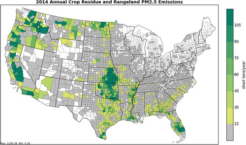
Figure 2. PM_2.5 ratio of 2014 annual crop residue and rangeland to 2011NEIv2 from all sources excluding crop residue burning.

Independent comparison with state-supplied data

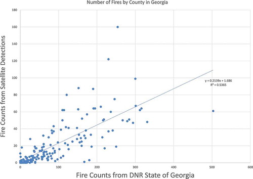
The Department of Natural Resources (DNR) from state of Georgia provided an independent set of crop and pasture fire locations for the year 2014. This data set was not based on satellite detections but on a subset of the burn permits for agricultural fires as small as 1 acre. These fires were accomplished burns, not just permitted. However, for fires less than 100 acres, exact fire locations were not provided, only the centroid of the county in which the fire occurred. In 2014, an annual total of 15,096 crop and pasture fires were reported by the state of Georgia. This number is significantly higher than the number of satellite detections because over 12,000 of these fires were smaller than 40 acres, too small to be detected by satellite. Since the satellite detections do not estimate the size of the fire, we can compare the Georgia DNR data set with our method in two ways: (1) the number of fire counts for each calendar day from both data sets and (2) the number of fires in each county over the year. Figure 3 shows a time series of the agricultural crop and pasture fires per day in the state of Georgia for the method described in this paper compared with the number reported by Georgia DNR. Figure 4 shows a scatter plot of the number of fire detections per county for all counties in Georgia that reported crop and pasture fires for the inventory year of 2014. Although the satellite detections are much lower than the number estimated from DNR, we see that there is some agreement both spatially at the county level (r = 0.73) and temporally to give some confidence in the satellite detections. We emphasize that data from only one state (Georgia) is insufficient to evaluate the accuracy of the method discussed in this work. If we had access to data from multiple states from different parts of the country, we would be able to better assess our method.

Figure 3. Comparison for fire counts by day for the state of Georgia.

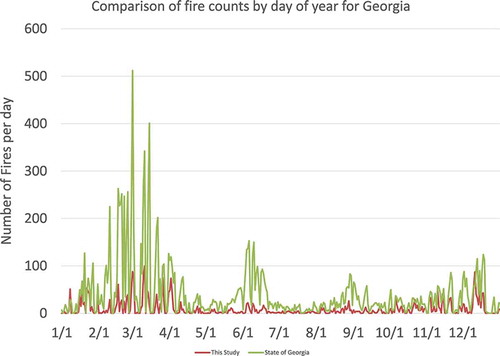
Figure 4. Fire counts by Georgia county satellite versus Georgia Department of Natural Resources.

Verification of diurnal activity pattern for crop residue burning

In air quality modeling, physical, chemical, and dynamic processes are modeled at time scales of minutes. The diurnal variation in meteorological parameters influences all these processes on a time scale on the order of minutes to hours. We must therefore have the best possible estimate of the diurnal variation of emissions in our air quality model to get the best model performance.

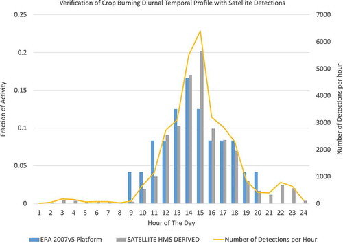
The HMS detection data includes the time of detection in Greenwich Mean Time (GMT) for each detected fire. Using the time of detection for all the nonduplicate fires and the assumed field size, and adjusting to local time from GMT, we were able to create a diurnal profile for the agricultural fires (excluding grass/pasture) based entirely on the satellite detections. This information was normalized by the number of acres per field across all hours and compared with the existing diurnal profile used in EPA’s modeling platform. Figure 5 shows the comparison between the satellite-derived profile and the profile in EPA’s 2007 modeling platform (figures 3–6 in EPA, 2012). We note that the satellite-derived profile is biased low between the hours of 9 a.m. and 12 p.m. and biased high for the last 4 hr of the day. We suspect that satellite data still contains some false detections or other inconsistencies, especially in the night time hours, to explain this high bias. The profile in EPA’s 2007 modeling platform was based on expert opinion rather than any measurement. We see some differences in the profiles between the hours of 9 a.m. and 12 p.m. However, these differences would not make a significant impact when used as part of a 12-km regional chemical transport modeling simulation in our opinion. Our reasoning is that at the regional scale of 12 km, the emissions are well mixed during the daytime hours within the boundary layer and so the exact timing of emissions allocated during the daytime hours would not change modeled concentrations. At finer scales, we would expect the temporal allocation to be more important and would recommend a more detailed approach to the allocation of emissions in a chemical transport model. We note that many of the nonfire diurnal profiles in the emission modeling platform do not have any ground-based measurements or expert opinion. This profile is one of the few with at least some comparison with independent data.

Figure 5. Verification of crop burning diurnal temporal profile with satellite detection.

Our estimates of both crop and rangeland burning emissions show that these emission sources have four main source regions: the southeastern United States, the lower Mississippi Valley, the Pacific Northwest and the Dakotas, and California. We have highlighted the difficulty in identifying fires detected by satellite because of limitations in the spatial accuracy of satellite detections. We have improved the inventory by using a consistent emission factors, and a set of satellite detections that capture the spatial and temporal variability of these emission sources. We have employed the best available emission factors in estimating emissions from crop residue burning and rangeland burning.

Summary

In this paper we have summarized a draft method for the 2014 NEI to estimate crop residue burning emissions and grass/pasture burning emissions using remote sensing data and estimated field size information. Comments from a number of states provided additional criteria for the identification of these fires from satellite detections. Specifically, when there is natural snow cover on the ground, crop residue burning is assumed to not occur. Additionally, in the midwestern states, we assume that the intentional burning of corn and soybean fields is very rare and do not consider fire detections near these crops to be crop residue burning but rather wildfires because of their accidental nature. The inputs as well as the state-level estimates used to create a national crop residue burning emission inventory for 2014 have been outlined and are available at http://www.epa.gov/sites/production/files/2015-06/draft_2014_ag_grasspasture_emissions_nei_may62015.xlsx. This method is easy, simple, and efficient. It can be easily applied across multiple years over the CONUS at minimal cost. For non-CONUS areas, the same methods can be applied if similar input data sets were to become available: land use by specific crop type, satellite detections, and appropriate emission factors.

Conclusion

Our estimation of the 2014 emission inventory for crop residue burning and rangeland burning shows that these sources of emissions have a unique spatial and temporal pattern. These emission sources occur in four main source regions: the southeastern United States, the lower Mississippi Valley, the Pacific Northwest and the Dakotas, and California. Using the best available input data sources of both satellite and field data, we can estimate this emission in an efficient way with minimal cost. Although satellite data provide important information about the location of a fire, other sources of data are need to accurately identify the type of fire. Satellite data can be used to estimate temporal patterns of emission sources when many detections are readily available. Future work would include the expansion of the method to multiple years, comparisons with burn area data from additional states, and updates to the emission factors.

Disclaimer

This paper has been reviewed in accordance with the U.S. Environmental Protection Agency’s peer and administrative review policies and approved for publication.

Supplemental data

Supplemental data for this article can be accessed on the publisher’s website.

Additional information

Notes on contributors

George Pouliot

George Pouliot is a physical scientist in the National Exposure Research Laboratory at the U.S. Environmental Protection Agency in Research Triangle Park, NC.

Venkatesh Rao

Venkatesh Rao is physical scientist in the Office of Air Quality Planning and Standards at the U.S. Environmental Protection Agency in Research Triangle Park, NC.

Jessica L. McCarty

Jessica L. McCarty is an adjunct assistant professor and a school of technology research scientist II at Michigan Tech Research Institute in Ann Arbor, MI.

Amber Soja

Amber Soja is an associate research fellow at the Institute of Aerospace, National Aeronautics and Space Administration Langley Research Center, in Hampton, VA.

References

- Akagi, S.K., R.J. Yokelson, C. Wiedinmyer, M.J. Alvarado, J.S. Reid, T. Karl, J.D. Crounse, and P.O. Wennberg 2011. Emission factors for open and domestic biomass burning for use in atmospheric models. Atmos. Chem. Phys. 11:4039–4072. doi:10.5194/acp-11-4039-2011.
- Akimoto, H. 2003. Global air quality and pollution. Science 302:1716–1719. doi:10.1126/science.1092666.
- Anderson, D.C., J.M. Nicely, R.J. Salawitch, T.P. Canty, R.R. Dickerson, T.F. Hanisco, G.M. Wolfe, E.C. Apel, E. Atlas, T. Bannan, S. Bauguitte, N.J. Blake, J.F. Bresch, T.L. Campos, L.J. Carpenter, M.D. Cohen, M. Evans, R.P. Fernandez, B.H. Kahn, D.E. Kinnison, S.R. Hall, N.R.P. Harris, R.S. Hornbrook, J. Lamarque, M. Le Breton, J.D. Lee, C. Percival, L. Pfister, R.B. Pierce, D.D. Riemer, A. Saiz-Lopez, B. J.B. Stunder, A. M. Thompson, K. Ullmann, A. Vaughan, and A. J. Weinheimer. 2016. A pervasive role for biomass burning in tropical high ozone/low water structures. Nat. Commun. 7:10267. doi:10.1038/ncomms10267.
- Brunekreef, B., and S.T. Holgate. 2002. Air pollution and health. Lancet 360:1233–1242. doi:10.1016/S0140-6736(02)11274-8.
- Jenkins, B.M., A. Daniel Jones, S.Q. Turn, and R.B. Williams. 1996. Particle concentrations, gas-particle partitioning, and species intercorrelations for polycyclic aromatic hydrocarbons (PAH) emitted during biomass burning. Atmos. Environ. 30:3825–3835. doi:10.1016/1352-2310 (96)00084-2.
- Keshtkar, H., and L.L. Ashbaugh. 2007. Size distribution of polycyclic aromatic hydrocarbon particulate emission factors from agricultural burning. Atmos. Environ. 41:2729–2739. doi:10.1016/j.atmosenv.2006.11.043.
- Larkin, N.K., T. Strand, R. Solomon, S. Raffuse, S. Drury, D. Sullivan, and L. Chinkin. 2010. Developing an improved wildland fire emissions inventory. Paper presented at American Geophysical Union Fall Meeting, San Francisco, CA, Dec 13–17.
- McCarty, J.L. 2011. Remote sensing-based estimates of annual and seasonal emissions from crop residue burning in the contiguous United States. J. Air Waste Manage. Assoc. 61:22–34. doi:10.3155/1047-3289.61.1.22.
- McCarty, J.L., S. Korontzi, C.O. Justice, and T. Loboda. 2009. The spatial and temporal distribution of crop residue burning in the contiguous United States. Sci. Total Environ. 407:5701–5712. doi:10.1016/j.scitotenv.2009.07.009.
- Pace, T., and G. Pouliot. 2007. Wildland fire National Emissions Inventory: Past, present and future. Paper presented at the 16th Annual International Emission Inventory Conference Emission Inventories: “Integration, Analysis, and Communications,” Raleigh, NC, May 14–17 2007.
- Pouliot, G., J.L. McCarty, A. Soja, and A. Torian. 2012. Development of a crop residue burning emission inventory for air quality modeling. Paper presented at the 20th EPA Emission Inventory Conference Emission Inventories—Meeting the Challenges Posed by Emerging Global, National, Regional and Local Air Quality Issues, Tampa, FL, August 13–16, 2012.
- Pouliot, G., T.G. Pace, B. Roy, T. Pierce, and D. Mobley. 2008. Development of a biomass burning emissions inventory by combining satellite and ground-based information. J. Appl. Remote Sens. 2:021501. doi:10.1117/1.2939551.
- Raffuse, S.M., D.A. Pryden, D.C. Sullivan, N.K. Larkin, T. Strand, and R. Solomon. 2009. SMARTFIRE algorithm description. U.S. Environmental Protection Agency, Research Triangle Park, NC. Prepared by Sonoma Technology, Inc., Petaluma, CA, and the US Forest Service, AirFire Team, Pacific Northwest Research Laboratory, Seattle, WA. STI-905517-3719.
- Ruminski, M., and J. Hanna. 2010. A validation of automated and quality controlled satellite based fire detection. American Geophysical Union Fall Meeting, San Francisco, CA, Dec 13–17.
- Ruminski, M., S. Kondragunta, R. Draxler, and J. Zeng. 2006. Recent changes to the Hazard Mapping System. Paper presented at the 15th International Emission Inventory Conference: Reinventing Inventories—New Ideas in New Orleans, New Orleans, LA, May 15–18, 2006.
- Skamarock, W.C., J.B. Klemp, J. Dudhia, D.O. Gill, D.M. Barker, M.G. Duda, H.-Y. Huang, W. Wang, and J.G. Powers. 2008. A Description of the Advanced Research WRF version 3. NCAR Tech Note NCAR/TN 475 STR. Boulder, CO: National Center for Atmospheric Research.
- United States Department of Agriculture. 2015a. USDA National Agricultural Statistics Service Cropland Data Layer for 2015. http://nassgeodata.gmu.edu/CropScape ( accessed April 1, 2015).
- Unites States Department of Agriculture. 2015b. USDA National Agricultural Statistics Service Cropland Data Layer Frequently Asked Questions. http://www.nass.usda.gov/research/Cropland/sarsfaqs2.html#Section4_3.0 ( accessed April 1, 2015).
- U.S. Environmental Protection Agency, Emissions, Monitoring and Analysis Division. 2003. Documentation for the Final 1999 Nonpoint Area Source National Emission Inventory for Hazardous Air Pollutants (Version 3). ftp://ftp.epa.gov/EmisInventory/finalnei99ver3/haps/documentation/nonpoint/nonpt99ver3_aug2003.pdf (accessed September 9, 2016).
- U.S. Environmental Protection Agency. 2012. Technical Support Document Preparation of Emission Inventories for the Version 5.0, 2007 Emissions Modeling Platform. https://www.epa.gov/sites/production/files/201510/documents/2007v5_2020base_emismod_tsd_13dec2012.pdf ( accessed September 9, 2016).
- U.S. Environmental Protection Agency. 2015. Draft Agricultural Burning Emission Estimates. http://www.epa.gov/ttn/chief/net/2014nei_files/draft_2014_ag_grasspasture_emissions_nei_may62015.xlsx ( accessed June 1, 2015).
- U.S. Environmental Protection Agency. 2016a. Technical Support Document Preparation of Emission Inventories for the Version 6.3, 2011 Emissions Modeling Platform. https://www.epa.gov/sites/production/files/201609/documents/2011v6_3_2017_emismod_tsd_aug2016_final.pdf ( accessed September 9, 2016).
- U.S. Environmental Protection Agency. 2016b. Green Book Nonattainment Area Summary. https://www3.epa.gov/airquality/greenbook/knsum.html ( accessed September 9, 2016).