A Monte Carlo method for summing modeled and background pollutant concentrations

ABSTRACT

Air quality analyses for permitting new pollution sources often involve modeling dispersion of pollutants using models such as AERMOD (American Meteorological Society/U.S. Environmental Protection Agency Regulatory Model). Representative background pollutant concentrations must be added to modeled concentrations to determine compliance with air quality standards. Summing 98th (or 99th) percentiles of two independent distributions that are unpaired in time overestimates air quality impacts and could needlessly burden sources with restrictive permit conditions. This problem is exacerbated when emissions and background concentrations peak during different seasons. Existing methods addressing this matter either require much input data, or disregard source and background seasonality, or disregard the variability of the background by utilizing a single concentration for each season, month, hour-of-day, day-of-week, or wind direction. Availability of representative background concentrations are another limitation. Here the authors report on work to improve permitting analyses, with the development of (1) daily gridded, background concentrations interpolated from 12-km CMAQ (Community Multiscale Air Quality Model) forecasts and monitored data. A two-step interpolation reproduced measured background concentrations to within 6.2%; and (2) a Monte Carlo (MC) method to combine AERMOD output and background concentrations while respecting their seasonality. The MC method randomly combines, with replacement, data from the same months and calculates 1000 estimates of the 98th or 99th percentiles. The design concentration of background + new source is the median of these 1000 estimates. It was found that the AERMOD design value (DV) + background DV lay at the upper end of the distribution of these one thousand 99th percentiles, whereas measured DVs were at the lower end. This MC method sits between these two metrics and is sufficiently protective of public health in that it overestimates design concentrations somewhat. The authors also calculated probabilities of exceeding specified thresholds at each receptor, better informing decision makers of new source air quality impacts. The MC method is executed with an R script, which is available freely upon request.

Implications: Summing representative background pollutant concentrations with air dispersion model output using a Monte Carlo method that respects the seasonality of each provides for more robust and scientifically defensible air quality analyses in support of permit applications. This work provides applicants a method to demonstrate compliance with National Ambient Air Quality Standards and avoid emission controls that might be based on overly conservative analyses. It also calculates the probability of exceeding the standard, allowing regulators to make more informed permitting decisions.

Introduction

When conducting air quality analyses in support of permit applications, regulators need to be sure that the new facility’s emissions, when added to current air quality conditions in the airshed, will not cause or contribute to an exceedance of any National Ambient Air Quality Standards (NAAQS). Regulators need access to accurate methods of predicting and evaluating the air quality impacts of proposed emissions. Such methods must be conservative enough to protect public health within the permitting process, but also realistic enough to permit new facilities where public health impacts will likely be minimal (Guerra et al., 2014).

Analyses of air quality impacts and NAAQS compliance are based on a metric known as the design value (DV). DVs are calculated according to a defined form and averaging time for direct comparison with each NAAQS. For instance, the primary 24-hr PM_2.5 (particulate matter with an aerodynamic diameter ≤2.5 μm) DV is computed by (1) calculating the 24-hr average concentration on each calendar day for three consecutive years, (2) calculating the 98th percentile of these 24-hr average concentrations for each of the three years, and (3) computing the average of the three 98th percentiles. The primary 1-hr sulfur dioxide (SO₂) DV is the 99th percentile of the daily maximum 1-hr concentrations per calendar year, averaged over 3 yr (40 C.F.R. § 50.4; National Primary and Secondary Ambient Air Quality Standards, 2015).

Regulatory models such as the American Meteorological Society (AMS) and U.S. Environmental Protection Agency’s (EPA) Regulatory Model (AERMOD) are run by applicants to estimate pollutant-specific air quality impacts caused by the proposed facility. To determine the future ambient pollutant concentration after the facility commences operations, modeled pollutant concentrations are added to measured or estimated background concentration data to derive a design concentration (DC) predictive of future DVs. If background concentrations do not adequately capture other nearby sources emitting substantial amounts of the same pollutants, their emissions must be included in the modeled inventory. A simplified conceptual diagram is provided in Figure 1.

Figure 1. Summing modeled and background concentrations during the permitting process.

Typically, the DVs of modeled AERMOD data (box 4, Figure 1) and background concentration data (box 5, Figure 1) are added together to derive a conservative DC estimate. This approach assumes a scenario in which the 98th (or 99th for SO₂) percentile concentration from the source and background occur simultaneously, although in reality their distributions are largely independent. Adding the 99th percentiles of two independent distributions is equivalent to choosing the 99.99th percentile of the combined distribution as the DC (Guerra, 2014). Although this can be considered a conservative approach that is more protective of public health, it could require unnecessarily restrictive emission controls.

The past few versions of AERMOD have allowed the inclusion of paired-in-time pollutant background concentrations with model-predicted pollutant concentrations, if the air quality monitor is adequately representative of recent background conditions in the area, and AERMOD is supplied with meteorological data from the same days as the background air quality monitor. However, it must be noted that model evaluation studies have demonstrated that AERMOD has low skill in predicting either paired-in-space or paired-in-time concentrations (Guerra, 2015; Murray and Newman, 2014). Further, these data requirements are rarely met during permit modeling; most applicants use existing preprocessed meteorological data to drive the AERMOD system. In spite of being a few years old, these meteorological data may still be representative of conditions in the area unless there have been significant changes to nearby terrain, structures, or land use. But it would not be correct to sum (paired-in-time) corresponding AERMOD output concentrations with background pollutant concentrations measured in different years.

AERMOD allows for seasonal, monthly, day-of-week, hour-of-day, or wind direction–specific pollutant background concentrations to be summed with model output. These options only accommodate a single background concentration from a particular direction, season, month, hour-of-day, or day-of-week. The inherent variability in background pollutant concentrations within these temporal or directional categories is not accounted for.

Although there is little published information on the subject, summing background pollutant and modeled pollutant concentrations to estimate DCs has been discussed at forums of state, local, and federal air quality regulators (Becker, 2008, 2010, and references therein; Guerra, 2015). Becker (2008) proposed including background emissions in the same AERMOD run as the facility being modeled. Although this method would yield more accurate DCs, the modeling process requires a large amount of input data. Guerra (2014) proposed adding modeled DVs with the median background concentration. This method is less conservative than the typical approach, although the assumption of a single background value year-round is oversimplified and incongruous with seasonal pollution patterns typically observed. Finally, Murray and Newman (2014) proposed summing all possible combinations of modeled and background data and calculating the 98th or 99th percentile of the resulting distribution. This probabilistic approach is less conservative than typical methods but also fails to respect seasonal differences between source and ambient concentration distributions.

An additional challenge in calculating accurate DCs is that representative background pollutant concentrations are often difficult to define, especially in unmonitored areas. Regulators often resort to using data from urban air quality monitors to estimate background pollutant levels at rural locations. Not only are these data likely to be overestimates, but also they may not have the correct seasonal fluctuations of ambient pollutant concentrations. This challenge, combined with the limitations of DC calculation methods discussed above, compromises the accuracy of air quality analyses conducted in support of permit applications.

This paper proposes a two-pronged approach to address these concerns: (1) develop daily gridded, representative background concentrations based on modeled and monitored data from a limited set of years; and (2) develop a Monte Carlo (MC) method to combine AERMOD output and background pollutant concentration data in a manner that respects the seasonality of their distributions. We present AERMOD performance data to justify this “paired-in-season” MC approach and proceed to evaluate the accuracy of the MC approach using simultaneous emissions, meteorology, and downwind monitoring data from a cluster of SO₂-emitting facilities in Washington State. Together, these two techniques allow for more accurate predictions of the air quality impacts of permitted facilities and more representative DCs.

Methods

Gridded daily PM_2.5, SO₂, and NO₂ concentrations

We developed maps of gridded daily background concentrations at a 12-km resolution across the Pacific Northwest states of Washington, Oregon, and Idaho for PM_2.5 (24-hr averages), SO₂ (daily 1-hr maxima), and nitrogen dioxide (NO₂; daily 1-hr maxima), as follows:

1. We extracted archived Community Multiscale Air Quality (CMAQ) model forecasts produced by Washington State University for years 2009–2011. Forecasts were driven by 12-km predicted meteorological fields from the University of Washington’s Mesoscale Model version 5 (http://www.atmos.washington.edu/mm5rt) and gridded emission data approximately corresponding to the 2005 EPA National Emissions Inventory. A full description of this CMAQ system and its performance is provided by Chen et al. (2008).

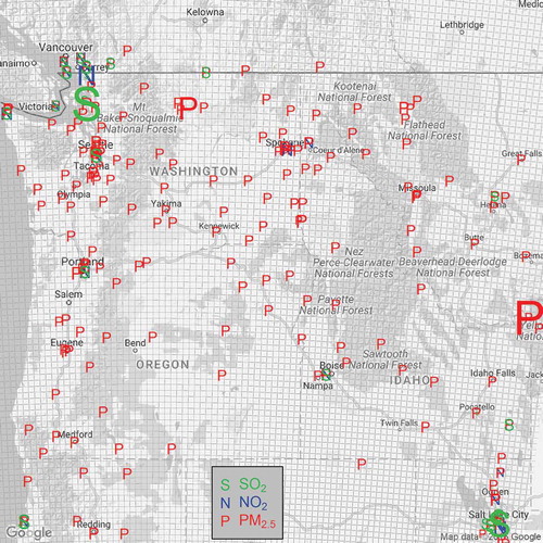
2. We obtained air quality monitoring data for the same period from EPA’s Air Quality System (AQS), state databases, and Canadian provincial authorities. We included monitoring data from bordering British Columbia, Montana, Wyoming, Utah, Nevada, and California sites to constrain any “edge effects” close to the domain boundary. Figure 2 shows all air quality monitors and the CMAQ domain used in this work. Sites containing fewer than 180 days of valid data within the 3-yr period and those disproportionately influenced by local sources not captured by CMAQ (e.g., compliance SO₂ monitors at smelting facilities and NO₂ data at a Canadian border post, which was heavily influenced by idling emissions) were not considered for this work.

3. We first paired each monitoring site with its corresponding CMAQ grid cell and calculated daily ratios of monitored/modeled concentrations. We log-transformed these ratios and interpolated them across the domain using Voronoi neighbor averaging (VNA), a deterministic modeling technique that identifies the nearest monitors to each grid cell and calculates the inverse-distance-weighted average of nearest monitors for each cell in the domain (Chen et al., 2004). The result of the VNA interpolation was the natural logarithm of a single monitored/modeled concentration ratio for each cell in the domain.

   The VNA approach is a well-established interpolation technique used in EPA’s Environmental Benefits Mapping and Analysis Program (BenMap) (EPA, 2008). Numerous applications of VNA in assessments of criteria pollutant health impacts have been described (Gronlund et al., 2015; Kim et al., 2014; Kheirbek et al., 2013; Fann et al., 2012; Grabow et al., 2012; Berman et al., 2012; Davidson et al., 2007). The average difference between VNA-predicted and observed ozone concentrations nationwide was found to be less than 1% with a standard deviation of 10–12%, as assessed by leave-one-out cross-validation, with lowest accuracy in remote rural areas (Hubbell et al., 2005). EPA also evaluated VNA for ozone interpolation in three U.S. cities (Atlanta, Detroit, and Philadelphia). The resulting gradients were able to predict monitored concentrations with correlation coefficients of 0.84–0.87 and mean bias of <1 ppb, although the predictive accuracy of VNA is expected to be lower outside of urban areas where monitoring networks are less dense. Although VNA introduced greater mean bias than more sophisticated modeling techniques such as Bayesian downscaling (EPA, 2014), we limited our evaluation to VNA because of its computational simplicity.

4. The VNA interpolation used inverse-distance-squared weighting for PM_2.5 ratios and inverse-distance weighting for SO₂ and NO₂ ratios, consistent with our conceptual understanding of patterns in spatial heterogeneity of these pollutants. Data from between one and seven neighboring sites out to a maximum distance of 250 km were used in the VNA interpolation of PM_2.5, whereas all available sites were used to interpolate NO₂ and SO₂. The antilog of the VNA result in each cell was

   Figure 2. Monitoring sites and 12-km CMAQ grids used in this work. Symbol sizes are proportional to mean two-step-interpolated/observed data (discussed later).

   
   multiplied by the same day’s gridded CMAQ concentration for that cell. See eq 1.

1

where N is the number of monitors considered to be neighbors of grid y, and IDW_|n,y| is the inverse-distance weight (or inverse-distance-squared weight for PM_2.5) of monitor n, at grid y. The VNA interpolation is shown inside the braces in eq 1.

Performing spatial interpolations on the natural logs of the monitor/model ratios helped to smooth unreasonably high interpolated values that occur when modeled values were low.

Monte Carlo combination of AERMOD output with daily pollutant background

We developed an original R function (R Core Team, 2014) to repeatedly sum with replacement randomly selected daily pollutant background concentrations, with AERMOD concentrations from within the same month. The R function randomly selects 31 days from all January days modeled with AERMOD, and 31 days from all January days for which background concentrations are available. It assembles 31 daily sums and then repeats this process for all months of the year. After assembling a single representative year of AERMOD + background data at each receptor, 99th percentiles are calculated at each receptor and stored. The whole process was repeated 1000 times, each time by selecting with replacement random data from within the same months. Bowman and Dhammapala (2011) found that the median of all the 98th or 99th percentiles provides a robust estimate of DCs and is unlikely to be influenced much by deviations from normality. A schematic of data flows is shown in Figure 3.

Figure 3. Schematic of Monte Carlo method to sum AERMOD and background data. For SO₂, x = 99; for PM_2.5 and NO₂, x = 98.

In addition to the medians, we also calculated the probability of the DC exceeding the NAAQS for each pollutant. When assessed in tandem with the median DC, this metric is indicative of the spread of the MC method output and is likely to be of use to decision makers. As the process accounts for seasonality and variability in modeled and background concentrations after a proposed facility commences operations, it is thought to provide a more realistic estimate of the DC.

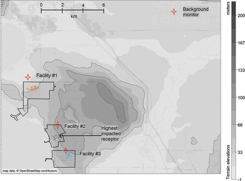
We were able to assess the accuracy of this MC method when a suitable data set from an unrelated AERMOD modeling project became available to us. That project modeled SO₂ from a cluster of three sources using 2012–2014 actual emission data, and on-site surface meteorological data from the same years. Background SO₂ concentrations from a monitor minimally impacted by these sources (AERMOD predicted a DV of 2 ppb at this monitor, but its measured SO₂ DV was 19 ppb) were combined with model output as illustrated in Figure 3. The resulting DCs were compared with SO₂ DVs measured immediately downwind of the three facilities, during the same time period. Figure 4 shows the layout of these sources and monitors. We did not use the gridded background concentration lookup tool described earlier, since emissions from these three sources were already included in CMAQ forecasts. As such, the 2009–2011 gridded concentrations in the vicinity of these facilities are not representative of background SO₂ levels in the absence of these sources.

Figure 4. Map of SO₂ sources and monitors used to test our Monte Carlo method. Monitors (red stars) within or very close to facility boundaries are treated as on-site monitors.

Results and discussion

Gridded background concentrations

Results of the daily gridded background interpolation are available to the public at http://www.lar.wsu.edu/nw-airquest/lookup.html. Users can download one date-stamped CSV file per pollutant, containing daily data between 1 January 2009 and 31 December 2011 by clicking on a location of interest.

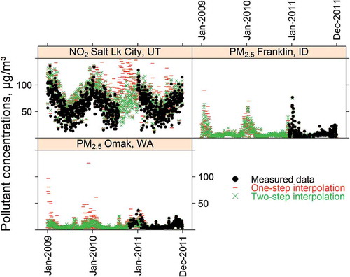
Although the interpolation mostly reproduced measured concentrations, not all instances with missing monitoring data were handled reasonably. This is illustrated by the differences in the red dashes (one-step interpolation) and filled black circles (measured data) in Figure 5. We only show the comparison at three sites for the sake of clarity. Missing periods were sometimes filled in with interpolated data that appeared to be from a distribution very different from the remainder of the time series (see NO₂ at Salt Lake City, UT, during the middle of the 3-yr period, for example). Some sites contained seemingly arbitrary spikes in the interpolated data (see PM_2.5 at Omak, WA, in early 2009) that were neither justified based on remaining observed data nor seen in the original CMAQ model output.

Figure 5. Comparison of 2009–2011 interpolated data against observations at selected sites.

Previous work (NW-AIRQUEST, 2013) found the interpolated solution was sensitive to the omission of certain monitors, particularly PM_2.5 monitors located in small constrained valleys. If a few such monitors fail to report data on a given day, the interpolated solution is less accurate because the 12-km CMAQ model is unable to properly characterize emissions and terrain in those areas.

We addressed this concern by first interpolating measured concentrations on a given day to locations that did not report valid data on that day. This computation is shown in eq 2. We used VNA interpolation with the same parameters described for eq 1 (1–7 neighbors within 250 km weighted by inverse distance squared for PM_2.5, all neighbors inverse-distance weighted for SO₂ and NO₂). This created a two-step interpolation routine, where missing monitoring values were first interpolated according to eq 2 (step 1) and domain-wide concentrations were then interpolated according to eq 1 (step 2). Step 1 guaranteed that all monitoring sites either retained their measured values or reported interpolated values on each of the 1095 days.

2

where monitor y is missing data on day i, N is the number of monitors considered to be neighbors of monitor y, and IDW_|n,y|is the inverse-distance weight (or inverse-distance-squared weight for PM_2.5) of monitor n at monitor y. We did not log-transform the monitor concentrations like the monitor/CMAQ ratios in eq 1.

Spatially interpolating monitoring data to fill in missing days is preferred over imputing missing data at each monitoring site. The latter approach—which considers each site in isolation—attempts to remain consistent with the site-specific data distribution when filling in missing data but risks ignoring regional episodes such as meteorological stagnation events that can cause elevated pollutant levels at several monitoring sites simultaneously.

The results of the two-step interpolation are shown by green “x” symbols in Figure 5. Although the two-step process made little difference at many sites and on many days, it appears superior to the single-step interpolation (red dashes) on several instances. On those occasions, the two-step interpolation is relatively free of abnormal spikes mentioned above, matches somewhat closer with the observations, appears to show the correct seasonality for the most part, especially when filling in missing data (compare black circles and green “x” data series for NO₂ at Salt Lake City, UT, and PM_2.5 at Franklin, ID, for example), and provides a more reasonable spatial pattern (spatial results not shown).

The symbol sizes in the map shown in Figure 2 are scaled by the mean two-step-interpolated/measured ratio at each site. A few sites were overestimated due to various reasons, but domain-wide comparison statistics for each pollutant shown in Table 1 indicate that the overestimate averages 6.2%. Although not directly comparable, this is well within the performance goal of ±30% for photochemical grid models simulating PM_2.5 (Boylan and Russell, 2006), which EPA uses.

Table 1. Evaluating domain-wide interpolation performance: Two-step-interpolated/observed ratios and confidence intervals.

Pollutant	All available data	Median of 10 iterations, each omitting 10% randomly selected sites
NO2	1.077 ± 0.101	0.878 ± 0.094
PM2.5	1.023 ± 0.026	1.024 ± 0.027
SO2	1.086 ± 0.229	1.156 ± 0.217
All	Mean = 1.062 ± 0.251	Mean = 1.019 ± 0.238

To further investigate the sensitivity of the interpolation to missing data, we conducted “leave some out” tests for each pollutant, by performing 10 repetitions of the two-step interpolation while withholding 10% randomly chosen monitoring sites for each pollutant. For example, during each of the 10 iterations, 18 randomly selected PM_2.5 sites were withheld and the two-step interpolation was performed on 167 sites, on 1095 days. The effect on the domain-wide comparison (rightmost column of Table 1) suggests that the extent of the error was within ±16%.

As stated earlier, the 12-km CMAQ model is unable to capture the spatial gradients in small communities. Further, although the “influence” of monitors is down-weighted by distance (for SO₂ and NO₂) or distance squared (for PM_2.5), VNA interpolation can extend the influence of some monitors beyond their natural boundaries. These limitations of our method likely require higher-resolution modeling and interpolation or kriging methods that limit the area represented by each monitor, by accounting for terrain and pollutant source regions.

Although the three years of data used to produce the interpolated map may not represent the most current air quality conditions in Washington, Oregon, and Idaho, data from these years were not unduly influenced by the kind of exceptional wildfires that occurred during the summers of 2012, 2014, and 2015. This work did not cover the remaining criteria pollutants (PM ≤10 μm [PM₁₀], carbon monoxide [CO], ozone [O₃], and lead [Pb]), as there is little demand for daily background concentrations of those pollutants within a permitting context. The clickable map at http://www.lar.wsu.edu/nw-airquest/lookup.html already provides their background DVs.

Monte Carlo simulation

The AERMOD project data that became available to us provided a unique opportunity to compare our MC method against actual measurements and other DC calculation methods. We used these data to first confirm that AERMOD was able to match seasonal patterns observed at on-site monitors. The boxplot in Figure 6 shows both AERMOD and observed concentrations at facility 2 rising together in the middle of the year, even though they differ in magnitude. Facility 1’s on- site monitor also shows a similar but less pronounced pattern. Since facility 3 often lies downwind of facility 2, there is no clear seasonal pattern in the observed and modeled concentrations. Overall, these comparisons lend credence to the assumption that a “paired-in-season” MC approach is viable.

Figure 6. Comparing the seasonality of AERMOD predictions versus observations at facility 2, using 2012–2014 SO₂ data.

In Table 2, the numbers within braces are DVs attributable to each facility (i.e., emissions from each facility modeled as separate AERMOD source groups). Based on the difference between own-source-group-only and cumulative modeling results at each facility (first row in Table 2), except for facility 3, which often lies downwind of facility 2, other on-site monitors were hardly influenced by emissions from neighboring sources.

Table 2. Assessing the performance of our Monte Carlo method.

	SO2 DV, ppb
Model	Facility 1	Facility 2	Facility 3
AERMOD DV [facility’s AERMOD source group]	10 [8]	91 [88]	19 [3]
Monitored background DV and median	19 and 5
AERMOD DV + background DV (MC %ile)	29 (97)	110 (99)	38 (100)
On-site monitor (MC %ile)	16 (2)	81 (1)	27 (33)
This Monte Carlo method ± confidence interval	22 ± 0.21	95 ± 0.34	28 ± 0.16
Guerra (2014b): AERMOD DV + background median (MC %ile)	15 (1)	96 (59)	24 (4)
Murray and Newman (2014): All AERMOD + background combinations (MC %ile)	23 (53)	97 (68)	28 (52)

Even though concentrations on row 1 of Table 2 do not include ambient background concentrations, facility 2’s own source group produced higher concentrations at the receptor coinciding with its on-site monitor (88 ppb) than the monitor itself recorded (81 ppb), suggesting that AERMOD overpredicted SO₂ levels. Although there is an element of conservatism intentionally built in to AERMOD (Rood, 2014), it was not as pronounced at facilities 1 (model-without-background = 8 ppb, measured = 16 ppb) and 3 (model-without-background = 3 ppb; 19 ppb from all modeled sources without background, measured = 27 ppb).

Notwithstanding the overprediction of SO₂ by AERMOD at facility 2, DCs produced by our MC method are closer to measured DVs than the traditional method of summing AERMOD DVs and background DVs. The 95% confidence intervals of our MC method are narrow, given the sample size of 1000. The percentiles at which each of these metrics occur in the distribution of the one thousand 99th percentiles are also shown within parentheses in Table 2.

Despite the conservatism built into AERMOD, the AERMOD DV + background median method proposed by Guerra (2014) produced slightly lower DCs than were measured by monitors at Facilities 1 and 3. As such, this method may not be adequately conservative, in that it underestimates concentrations that the public is exposed to. It remains to be seen if the extent of underestimation would change much in a different case study. The 99th percentiles of all AERMOD + background combinations proposed by Murray and Newman (2014) were within a few ppb of our MC method and fall relatively close to the median of the one thousand 99th percentiles. However, it must be reiterated that both these statistical methods proposed in the literature do not respect the seasonality of source emissions and background concentrations. In this particular example, measured background SO₂ concentrations did not exhibit large seasonal differences. The difference between our MC method and the others would have been more pronounced in a situation where, for example, AERMOD was run on a lumber kiln that increased production and therefore its PM_2.5 emissions during summer months, and the facility was located in a community with impaired air during wintertime due to wood burning for home heating.

To confirm if the median of all one thousand 99th percentile estimates is an appropriate metric for this application, we examined their distributions at the three facilities’ on-site monitors and at the most impacted receptor in the AERMOD modeling domain. Figure 7 shows density plots at each of these four receptors, overlaid with their medians (vertical dashed black line), AERMOD DV + background DV (rightmost vertical red line), measured DVs (vertical dotted green line), 99th percentiles of all AERMOD + background combinations (Murray and Newman, 2014; vertical blue line), and the AERMOD DV + median background (Guerra, 2014; vertical gray line). Quantile plots (not shown) and the Shapiro–Wilcox test confirm these 1000 estimates of DCs are normally distributed.

Figure 7. Density plots of 1000 estimates of SO₂ 99th percentiles, produced by this Monte Carlo method.

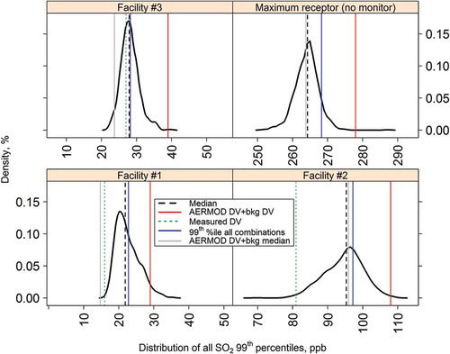
In this example, the AERMOD DV + background DV lies at the upper end of the distributions of one thousand 99th percentiles whereas the measured DV is mostly at the lower end. Our MC method sits between these two metrics and can be considered somewhat more protective of public health in that it slightly overestimates DCs, but not overly so. Further, the availability of 1000 estimates allows the computation of the probability of a NAAQS exceedance (i.e., the fraction of all 1000 DC estimates, which are higher than the NAAQS), a metric that is likely to be of interest to air quality planners. Facility 2 has a 99.9% probability of exceeding the SO₂ NAAQS, whereas the other two facilities have 0% probability. The most impacted receptor in the modeling domain has a 100% probability of an exceedance.

There may be certain conditions under which high AERMOD concentrations and background concentrations are expected to co-occur within the same month, more often than by chance. For example, depending on stack characteristics, higher levels of pollution from both permitted facilities and background sources could be expected simultaneously during a winter stagnation event. A MC scheme that treats both distributions as truly independent may underestimate the likelihood of an exceedance when high-pollution conditions co-occur. However, this limitation is partially mitigated by repeatedly pairing AERMOD and background data from randomly chosen days within the same month. It is very likely that there will be at least a few iterations with co-occurring high-pollution conditions.

With the availability of gridded background values, even facilities without background monitoring data can use this MC approach to achieve more accurate DCs in the permitting process.

Conclusion

This paper describes the development of an improved method for estimating air quality impacts from proposed facilities for three important criteria pollutants. This method includes calculation of daily background concentrations of PM_2.5, SO₂, and NO₂ throughout Washington, Oregon, and Idaho on a 12-km grid. Archived daily CMAQ forecasts were interpolated with all available monitoring data from 2009 to 2011, and the resulting background concentrations are provided via a clickable online map.

We proceeded to develop a Monte Carlo method for combining AERMOD output with suitable background data, irrespective of whether the latter were obtained directly from representative monitors or from the online interpolated map. To respect seasonal differences in facility emissions and ambient background, random sampling (with replacement) of AERMOD and background data occurred within the same month. At least three years of background and AERMOD data are recommended to account for annual fluctuations in meteorology and nearby emissions. AERMOD does not necessarily need to be run over the same years or duration as the background data.

The MC method does have some conservatism built in, in that it sums daily maxima of AERMOD and background NO₂ and SO₂ concentrations even if respective maxima occur at different hours during the same day. Testing showed this MC method produced DCs that were lower than the more conservative method of summing AERMOD DVs + background DVs, but were slightly higher than measured, postconstruction on-site DVs, thus providing a sufficiently conservative estimate of public exposure.

The probability of exceeding the NAAQS is a new metric that can be used to make more informed regulatory decisions. For instance, additional emission controls could be required if the proposed facility’s PM_2.5 DC is only 33 µg/m³ but has a 50% probability of exceeding the NAAQS.

The states of Washington, Oregon, and Idaho will use this technique in their minor New Source Review (NSR) programs as needed. We recommend the use of this Monte Carlo method in air quality analyses that are conducted nationwide, in support of permit applications. The R script we developed is available free of charge by contacting the authors. A software package is being prepared for submission to the Comprehensive R Archive Network (CRAN, 2016).

Acknowledgment

The authors gratefully acknowledge support and feedback provided by modelers and permit engineers at Idaho’s and Oregon’s respective Departments of Environmental Quality. Washington State University provided a Web server for hosting the background concentration map application. AERMOD data from a separate project made available to the authors by a consultant proved very helpful for evaluating the performance of the authors’ Monte Carlo method. Mr. Ralph Morris of Ramboll-Environ kindly volunteered to present this work at an AWMA conference when the authors were unable to attend. The manuscript also benefited from feedback provided by three anonymous reviewers.

Additional information

Notes on contributors

Ranil Dhammapala

Ranil Dhammapala, Clint Bowman, and Jill Schulte are atmospheric scientists at the Washington State Department of Ecology in Olympia, WA.

References

- Becker, D.L. 2008. PM2.5 NAAQS modeling—challenges & possible solutions. Presentation at the 23rd Annual Conference on the Environment—Upper Midwest Section of the AWMA, Minneapolis, MN, November 6. https://www.pca.state.mn.us/sites/default/files/airmodeling-presentation-1108.pdf (accessed January 10, 2017).
- Becker, D. 2010. Pairing Monitored Background and Modeled Data. Presentation at EPA Regional/State/Local Modelers Workshop, Portland, Oregon. http://www.cleanairinfo.com/regionalstatelocalmodelingworkshop/archive/2010/Documents/Presentations/Pairing%20Monitored%20Background%20and%20Modeled%20Data%20for%20PM2.5%20–%20May2010.pdf (accessed January 10, 2017).
- Berman, J.D., N. Fann, J.W. Hollingsworth, K.E. Pinkleton, W.N. Rom, A.M. Szema, P.N. Breysse, R.H. White, and F.C. Curriero. 2012. Health benefits from large-scale ozone reduction in the United States. Environ. Health Perspect. 120:404–1410. doi:10.1289/ehp.1104851
- Bowman, C., and R. Dhammapala. 2011. A Monte Carlo approach to estimating impacts from highly intermittent sources on short term standards. Presentation at NW-AIRQUEST annual meeting, Pullman, WA, June 1–3. http://www.lar.wsu.edu/nw-airquest/docs/201106_meeting/20110601_mc4intermittent_sources.ppt (accessed January 10, 2017).
- Boylan, J.W., and A.G. Russell. 2006. PM and light extinction model performance metrics, goals, and criteria for three-dimensional air quality models. Atmos. Environ. 40:4946–59. doi:10.1016/j.atmosenv.2005.09.087
- Chen, J., R. Zhao, and Z. Li. 2004. Voronoi-based k-order neighbor relations for spatial analysis. ISPRS J. Photogramm. Remote Sens. 59:60–72. doi: 10.1016/j.isprsjprs.2004.04.001
- Chen, J., J. Vaughan, J. Avise, S. O’Neill, and B. Lamb. 2008. Enhancement and evaluation of the AIRPACT ozone and PM2.5 forecast system for the Pacific Northwest. J. Geophys. Res. 113:D14305. doi:10.1029/2007JD009554
- Comprehensive R Archive Network (CRAN). 2016. https://cran.r-project.org (accessed January 10, 2017).
- Davidson, K., A. Hallberg, D. McCubbin, and B. Hubbell. 2007. Analysis of PM2.5 using the environmental benefits mapping and analysis program (BenMAP). J. Toxicol. Environ. Health Part A 70:332–46.
- Fann, N., A.D. Lamson, S.C. Anenberg, K. Wesson, D. Risley, and B.J. Hubbell. 2012. Estimating the national public health burden associated with exposure to ambient PM2.5 and ozone. Risk Anal. 32:81–95. doi:10.1111/j.1539-6924.2011.01630.x
- Grabow, M.L., S.N. Spak, T. Holloway, B. Stone Jr., A.C. Mednick, and J.A. Patz. 2012. Air quality and exercise-related health benefits from reduced car travel in the midwestern United States. Environ. Health Perspect. 120:68–76. doi:10.1289/ehp.1103440
- Gronlund, C.J., S. Humbert, S. Shaked, M.S. O’Neill, and O. Jolliet. 2015. Characterizing the burden of disease of particulate matter for life cycle impact assessment. Air Qual. Atmos. Health 8:29–46. doi:10.1007/s11869-014-0283-6
- Guerra, S. 2014. Practices to achieve a reasonable level of conservatism in AERMOD modeling demonstrations. EM 12:24–9. http://pubs.awma.org/gsearch/em/2014/12/guerra.pdf (accessed January 10, 2017).
- Guerra, S. 2015. Background concentrations and the need for a new system to update AERMOD. Presentation at 11th EPA Conference on Air Quality Modeling, Research Triangle Park, NC, August 12–13. http://www3.epa.gov/ttn/scram/11thmodconf/presentations/3-7_Background_Concentrations-CPP-11thMC.pdf (accessed January 10, 2017).
- Guerra, S.A., S.R. Olsen, and J.J. Anderson. 2014. Evaluation of the SO2 and NOx offset ratio method to account for secondary PM2.5 formation. J. Air Waste Manage. Assoc. 64:265–71. doi:10.1080/10962247.2013.852636
- Hubbell, B.J., A. Hallberg, D.R. McCubbin, and E. Post. 2005. Health benefits from large-scale ozone reduction in the United States. Environ. Health Perspect. 113:73–82. doi:10.1289/ehp.7186
- Kheirbek, I., K. Wheeler, S. Walters, D. Kass, and T. Matte. 2013. PM2.5 and ozone health impacts and disparities in New York City: Sensitivity to spatial and temporal resolution. Air Qual. Atmos. Health 6:473–86. doi:10.1007/s11869-012-0185-4
- Kim, Y.-M., Y. Zhou, Y. Gao, J.S. Fu, B.A. Johnson, C. Huang, and Y. Liu. 2014. Spatially resolved estimation of ozone-related mortality in the United States under two Representative Concentration Pathways (RCPs) and their uncertainty. Clim. Change 128:71–84. doi:10.1007/s10584-014-1290-1
- Murray, D.R., and M.B. Newman. 2014. Probability analyses of combining background concentrations with model-predicted concentrations. J. Air Waste Manage. Assoc. 64:248–54. doi:10.1080/10962247.2013.846282
- National Primary and Secondary Ambient Air Quality Standards. 2015. Code of Federal Regulations, Title 40, Part. 50.4.
- NW-AIRQUEST. 2013. Document detailing Overall Methodology of background design value lookup tool. http://www.lar.wsu.edu/nw-airquest/docs/3state_bg_conc_maps_methodology.pdf (accessed January 10, 2017).
- R Core Team. 2014. R: A language and environment for statistical computing. R Foundation for Statistical Computing, Vienna, Austria. http://www.R-project.org/ (accessed January 10, 2017).
- Rood, A.S. 2014. Performance evaluation of AERMOD, CALPUFF, and legacy air dispersion models using the Winter Validation Tracer Study dataset. Atmos. Environ. 89:707–20. doi:10.1016/j.atmosenv.2014.02.054
- U.S. Environmental Protection Agency. 2008. BenMap User Manual Appendices, Section C.3.3. https://www.epa.gov/sites/production/files/2015-07/documents/dec2009_benmapappendicessept08.pdf (accessed January 10, 2017).
- U.S. Environmental Protection Agency. 2014. Health Risk and Exposure Assessment for Ozone. https://www3.epa.gov/ttn/naaqs/standards/ozone/data/20140829healthrea.pdf (accessed January 10, 2017).