Urban heat island (UHI) influence on secondary pollutant formation in a tropical humid environment

ABSTRACT

The combined action of urbanization (change in land use) and increase in vehicular emissions intensifies the urban heat island (UHI) effect in many cities in the developed countries. The urban warming (UHI) enhances heat-stress-related diseases and ozone (O₃) levels due to a photochemical reaction. Even though UHI intensity depends on wind speed, wind direction, and solar flux, the thermodynamic properties of surface materials can accelerate the temperature profiles at the local scale. This mechanism modifies the atmospheric boundary layer (ABL) structure and mixing height in urban regions. These changes further deteriorate the local air quality. In this work, an attempt has been made to understand the interrelationship between air pollution and UHI intensity at selected urban areas located at tropical environment. The characteristics of ambient temperature profiles associated with land use changes in the different microenvironments of Chennai city were simulated using the Envi-Met model. The simulated surface 24-hr average air temperatures (11 m above the ground) for urban background and commercial and residential sites were found to be 30.81 ± 2.06, 31.51 ± 1.87, and 31.33 ± 2.1ºC, respectively. The diurnal variation of UHI intensity was determined by comparing the daytime average air temperatures to the diurnal air temperature for different wind velocity conditions. From the model simulations, we found that wind speed of 0.2 to 5 m/sec aggravates the UHI intensity. Further, the diurnal variation of mixing height was also estimated at the study locations. The estimated lowest mixing height at the residential area was found to be 60 m in the middle of night. During the same period, highest ozone (O₃) concentrations were also recorded at the continuous ambient air quality monitoring station (CAAQMS) located at the residential area.

Implications: An attempt has made to study the diurnal variation of secondary pollution levels in different study regions. This paper focuses mainly on the UHI intensity variations with respect to percentage of land use pattern change in Chennai city, India. The study simulated the area-based land use pattern with local mixing height variations. The relationship between UHI intensity and mixing height provides variations on local air quality.

Introduction

Extreme temperatures in urban hotspots are becoming more common worldwide. Rapid urbanization leads to high raised buildings and surface modifications in the city areas. The surface modifications and heavy trafficking exhaust emissions in the cities make them hotter than the surrounding suburban or rural areas; this phenomenon is called urban heat island effect (UHI). This effect was stronger in cold countries like Canada. It was reported that in Canada the number of days with average temperature above 30ºC was increased significantly (Rizwan et al., 2008; Memon et al., 2009). The raise in UHI intensity significantly affects the outdoor thermal comfort, energy usage, and air quality. The impact of land use change is an important parameter for local air quality estimations. Due to complexity in the urban building structure, resistance to the heat waves and wind velocity occur at a height below the average building height in the urban area. The solar radiation flux over different surface materials depends on the thermophysical properties. The albedo of pavement materials in the urban area has a significant effect on daytime temperature differences in the urban environment. It is reported that a high albedo of urban pavements reduces the UHI intensity during the daytime, but it does not affect nighttime temperatures. Apart from the natural heating systems in urban areas, heat emissions from anthropogenic sources like the transportation sector, indoor heating due to cooking, air conditioning, and other household activities play a significant role in increasing the local temperature profiles. In the past, several computational fluid dynamics (CFD) model studies were attempted to represent the diverse phenomena of UHI by implementing the complexity. They include the energy balance of solar energy, urban ventilation, health impacts, spatial and temporal variations of UHI intensities, and pollutant transformations.

The sky view factor (SVF) in the urban environment is the most important factor for solar energy trapping, and during typical summer days, it contributes to the rise in UHI intensity. The intensity of UHI depends on the SVF; it is high for high-SVF areas, whereas it is low for areas with a low SVF factor due to a shading effect, which moderates the UHI intensity (Wang et al., 2016).

During recent years, microscale models have gained importance for modeling the surface-layer interactions with the surrounding environment (Mirzaei, 2015). Deterministic models such as building energy models (BEM) developed based on the interactions of building volume with the surrounding environment, and several such CFD models developed based on the BEM model, microclimatic models (MCM), and the urban canopy model (UCM) were widely used to understand the UHI phenomenon. Statistical models like the artificial neural network and regression analysis were also used to correlate the UHI phenomena with characteristics of the city (Mirzaei, 2015). Models coupled with the surface energy balance and velocity component represent surface convection of various building materials used for determining the UHI phenomenon. The Envi-Met model can predict the diurnal thermal circulations using global solar fluxes for solving the energy balance equations. Countries in an underdeveloped stage are facing a heat-wave problem due to lack of mitigation technology in the city planning.

In the past, several studies suggested major mitigation strategies like the green roof, and enhanced albedo properties of surface materials like pavement and building materials. The effect of wind velocity on air temperature is an important parameter in studying the influence on UHI intensity and has not been explored in the past. These variations in air temperature lead to a change in mixing height due to changes in the environmental lapse rate. The average mixing height for each study region with different land use is a potential parameter for air quality management.

In this study, Envi-Met model simulations were made to understand the relationship between UHI intensity and changes of local meteorological parameters like air temperature, relative humidity (RH), and mixing height at selected locations in a tropical urban environment (Chennai city). The correlation between the meteorology and local air quality was also investigated.

Urban characteristics and UHI

Urban microenvironment structure

Most of the cities in India are growing rapidly due to a large number of people migrating from the rural and semi-urban areas. Typical urban zones in India consists of 80–85% land use as asphalt and concrete surface in which about 30% is asphalt and 50% is concrete. Asphalt and concrete are low-albedo materials, efficient in reflecting the incoming solar radiation. In addition to the pavement effect, the absence of vegetation in urban zones intensifies the UHI intensity, due to lack of shadow effect, evapotranspiration, and reflection (due to high albedo) of sunlight falling. The net radiation absorbed by surface materials is the difference between received solar radiation and the outgoing radiation. The energy-balancing equation (Wang et al., 2015, 2016). for each surface material is given by

(1)

where Q_{sw, net} is the net shortwave radiation at the surface, Q_lw,net(To) the net longwave radiation at the surface, G the soil heat flux, H the sensible heat flux, and LE the latent heat flux. In the past, for determination of UHI intensity based on land use change, many studies used the microclimatic models. With those models, they considered only the thermophysical surface material properties of various land uses for energy balancing.

Energy balancing models are being widely used for determining the UHI intensity in microscale modeling. However, coupled energy balancing and velocity component models are not popular for UHI determination (Toparlar et al., 2015).

Seasonal variations of meteorological parameters have significant effects on local temperature and pollution levels. Significant variation of mixing height depends on the wind speed and pressure gradient in local atmospheric condition. It is important to explore the impact of land use change on local meteorological properties like temperature, humidity, and mixing height at microscale level (Zhao et al., 2011). To capture the UHI intensity with land use change in three locations in Chennai city, four velocity conditions for each location were simulated.

UHI impact of local meteorology and air quality

Heavy traffic emissions, poor dispersion, and regional transport of pollutants make the air quality worse in the urban areas. Dispersion conditions in these areas play a significant role in primary and secondary pollutant concentrations. In the United States, it was reported that boundary-layer suppression causes pollutants to be trapped close to the surface (Zhao et al., 2011). In coastal regions, the marine atmospheric boundary layer (MABL) and ocean upwelling affect the local air pollution. Global climatic simulations have shown that temperature, humidity, and boundary-layer depth can cause changes in local air quality (Mahmud et al., 2008; Tagaris et al., 2007). Local ozone concentrations are well correlated with the temperature profile in California. Ozone and PM_2.5 formations simulated with changes in emission levels with MM5, SMOKE, and CMAQ models, NOx emissions, and biogenic volatile organic compound (VOC) emissions reductions result in reduced ozone (O₃) concentrations. One of the studies suggested that high temperature and VOC emissions will be responsible for high PM_2.5 (particulate matter of diameter 2.5 µm or less) concentrations in the future (Lioa et al., 2007).

UHI phenomenon in India

Chennai is a coastal city located in the southern part of India, with tropical climatic conditions, and has faced rapid urbanization during last two decades, from 1995 to 2015.

The city spreads over a 500-km² area with population of approximately 10 million. The average summertime ambient temperature during the day is increasing compared to the last decade. The mean of maximum temperatures is increasing in about 95% of the south Indian region. Each year 1200 people die as a result of heat-stress-related diseases in south India (World Health Organization [WHO], 2009). The potential increase in the local temperature profile as a result of rapid industrialization, high population density, and vehicular emissions was reported in past studies in Tamil Nadu state, India.

UHI effect on Ozone (O₃) concentration

Anthropogenic heat and local induced thermal circulations are strongly associated with the ozone (O₃) concentration in the urban environment. There is no comprehensive study for the relative effect of diurnal temperature on ozone concentration. Ryu et al. (2013a) concluded that a heat island effect with the change in land use and anthropogenic heat sources in urban areas influences the local temperature profiles. Ozone (O₃) formation is a complex phenomenon that also depends on meteorological parameters and local emissions. In this study we indicated that the increase in O₃ concentration was correlating with UHI intensity; similar observations were also reported by others (Sarrat et al., 2006; Jenkin and Clemitshaw, 2000).

Apart from the primary pollutant concentrations, secondary pollutants like ozone concentration depend on the intensity of temperature. Local temperature profiles will enhance O₃ transformations during nighttime. Recent studies of UHI effect on ozone concentration concluded that daytime formation of O₃ was affected by thermally induced air circulation and NOx dilution due to a change in boundary-layer height (Li et al., 2016).

Ozone concentration will be high at midday when sunlight will prevail in photochemical formation. During the nighttime, O₃ concentration depends on local temperature. It was concluded (Ryu et al., 2013b) that the concentration of O₃ was high during nighttime because the destruction of O₃ reaction is not effective during nighttime and due to the dilution effect of NOx. However, during daytime, the dilution effect and intensity of temperature contribute to increased O₃ concentrations. Ozone concentrations using the WRF chemistry model with urban and nonurban conditions (Ryu et al., 2013b) concluded that O₃ concentrations are higher during nighttime in urban simulations than in nonurban ones. During daytime the simulated O₃ concentration was low.

Methodology

Selection of study regions

Three locations representing different land use types in Chennai city, each with a 900 m × 900 m area, were selected. Microclimatic conditions for these areas were studied for May–June 2016. The microclimatic simulations were calculated with grid dimensions of 10 × 10 × 2 m. The present canyon land use, building height, building density, and vegetation were characterized for each area. The commercial area includes a large number of buildings with various building heights; in fact, in recent years several high-rise apartment towers have been constructed in this area. The residential area comprises a typical suburban land use pattern located very near to the coast. The background area conserves, with minimum land use change with scattered buildings. This area was a thick forest with an average tree height of 10 m. Figure 1 shows top views of the study areas having estimated sky view factors (SVF) of 0.357, 0.546, and 0.711 for background, commercial, and residential sites, respectively.

Figure 1. Chennai area map with three selected areas for the study, using yhe Envi-Met model: (a) IITM background site, (b) T Nagar commercial site, and (c) Royapuram residential site.

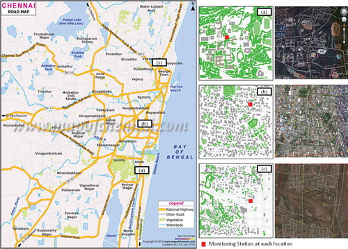
Figure 1 describes the three locations selected for the present study. For the background site the latitude and longitude are 12.9915° N, 80.2337° E; the commercial (T Nagar) area is located at 13.0405° N, 80.2337° E; and the residential site has latitude and longitude 13.1136° N, 80.2961° E. Here the areas are represented in the figure as (a), (b), and (c), as background, residential, and commercial sites respectively. The gray shadings in the figure indicate the building locations with various heights in each area file, and green shading indicates trees with 10 and 15 m height with different leaf area density (LAD). At the background site in total 37 buildings were presented in a selected 1-km² area, whereas this number was 317 at residential site and 386 at commercial site. The average building height was found to be 6 to 9 m at every location, that is, two-story and three-story buildings. At the commercial site, the building height was 15 to 18 m, and buildings were relatively closer than in the other two selected sites. Vehicular emissions are the main sources at all three selected study regions. Two wheelers, four wheelers, and trucks were the major contributors to local air pollution in Chennai city.

Urban microenvironment simulations

The Envi-Met model setup was for 900 × 900 × 55 (L × L × H) m for modeling the UHI at selected locations. Land use, building height, and building density at each study location were analyzed using ArcGIS. The population density was not included in the present study and the building materials were classified basically into walls and roof, uniform for all buildings. The thickness of walls and roof are classified into three layers, each layer of 10 cm with total width of 30 cm. The density of the concrete material used for wall construction and roof was 2000 and 2500 kg/m³, respectively.

The Envi-Met model (envi-met.com) can simulate with a spatial resolution of 0.5 m to 10 m and temporal resolution at 10 sec. This model is capable of simulating the various land use patterns and simulating the diurnal variations of local meteorological parameters. The area input file for Envi-Met simulation is with three-dimensional (3D) geometry, representing the study area characteristics of building structure, building height, and land use availability. The advantage of using this model is considering the energy balance and flow model simultaneously at microscale. Envi-Met is a 3D micrometeorological model that can simulate the microscale thermal interactions of various urban surface materials, with the surface–plant–air interactions, and has been extensively used and validated by many researchers in recent years. It can take into account shortwave radiation and longwave radiation fluxes, and shading effects of buildings and building materials. Reflection, reradiation, and evapotranspiration of different land use parameters are also considered for microclimatic simulations. The advantage of the Envi-Met model is that it can simulate the energy balance and velocity components for fluid flow and convective heat transfer for different surface materials (Toparlar et al., 2015). In most of the microscale (less than 10 km area for study) simulations, a ground roughness factor, which is a function of building height and structure, influences the local wind speed, wind direction, and temperature dissipation and was not incorporated. And in most of these, the model’s soil wetness and leaf area density (LAD) at the study area were not be considered. However, it was possible to consider these parameters using Envi-Met model simulations. ASTM building material and surface land use material properties considered for the present study are given in Table 1. Various building heights and land use changes were considered for simulation.

Table 1. Thermophysical properties of the materials.

Material	Absorption	Reflection (albedo)	Emissivity	Specific heat (J/kg-K)	Thermal conductivity (W/m-K)
Wall surface	0.7	0.3	0.9	840	0.85
Roof concrete surface	0.7	0.3	0.9	840	1.3
Loam soil	—	0.3	0.98	750	0.2
Asphalt road	0.6	0.4	0.9	650	1.16

Typical summer days, that is, May 15 to June 15, 2016, were selected for simulations. The 1-hr average data of two weather-monitoring stations located in a residential site and a background site were used as input to the Envi-Met model. At these monitoring stations, measurements were made at 10 m above the ground level, and are not affected by average building height in these areas. For a typical summer day, the maximum air temperature was found to be 35.5ºC at 12.00 hr IST, and the minimum was 30.7ºC at 5.00 hr IST.

Meteorology and air quality monitoring

In an attempt to determine the UHI intensity in Chennai city, in situ ambient meteorological monitoring was carried out at the selected study regions. Temperature, wind speed, and wind direction for the specified period were recorded for 1 week at each location. Air quality and meteorological parameters were measured with standard instrumentation suggested by the U.S. Environmental Protection Agency (EPA). A windmill anemometer was used for wind speed, a vane for wind direction, and a thermocouple sensor for temperature measurements. These instruments are attached to the data logger for storage of 1-hr average data.

Air quality measurements were conducted with the mobile monitoring station, from May 15 to 30 at the residential site and June 1 to 15 at the background site, with 1 hr frequency. Air quality monitoring at the commercial site was not performed, and only meteorological measurements were monitored during the same period in commercial site.

A t-test for paired observations was applied to identify the impact of wind speed on diurnal temperature variations.

Mixing height calculations

During daytime, mixing height can be estimated as an intersection of environmental lapse rate (ELR) and dry adiabatic lapse rate (DARL). ELR was chosen as the pre-sunrise vertical inversion profile. DALR was calculated at each time potential air temperature.

Model results were validated with the monitoring results at the same locations for temperature and RH. Mixing height resulting from simulations was compared with the average mixing height profiles given by the regional meteorological department for Chennai.

Results and discussion

Characterization of air temperature and humidity measurements

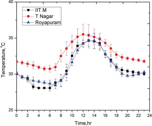
The mobile ambient air quality monitoring van was used to monitor ambient air temperature, relative humidity (RH), and ozone (O₃) concentrations at selected study regions in Chennai city. Figure 2 presents the comparison of diurnal temperature profiles at the selected study regions in Chennai city. Results indicated a maximum temperature of 34.66 ± 0.8ºC, 35.5 ± 1.4ºC, and 34.65 ± 1.02ºC at background, commercial, and residential sites, respectively, during the afternoon (between 12 noon and 2 p.m.).

Figure 2. Monitoring results of diurnal temperature profiles at selected study regions.

Envi-Met model results

Envi-Met simulations were initiated in the morning at 8 a.m. with initial temperature of 30.8ºC for the summer weather scenario with the cyclic boundary condition. Input for the simulations required wind velocity at 10 m height and RH at 2 and 2500 m height; all these data were taken from a weather station and also from radio sounding data (http://weather.uwyo.edu/upperair/sounding.html). Simulations were made for four velocity profiles, that is, 0.2, 1, 2, and 5 m/s, at each study area. Figure 3 shows the modeling of ambient air temperature profiles for different velocity conditions at the selected study locations. At the urban background site (Indian Institute of Technology [IIT] Madras) the simulated average ambient air temperatures for the four velocities were found to be 31.29, 31.3, 30.8, and 30.6ºC, respectively. The diurnal temperature profile indicated a maximum of 36.05ºC at 1 m/sec wind velocity condition for 1 p.m. (afternoon). The average diurnal ambient air temperature profile for the commercial site (T Nagar) with four velocity profiles (0.2,1, 2, and 5 m/s) was found to be 31.7, 31.6, 31.4, and 31.1ºC respectively. The intensity of average air temperature varies with the wind speed; an increase in wind speed up to 2 m/sec increases the UHI intensity, and it was decreased at 5 m/sec wind velocity condition. This is because at 0.2 m/sec only natural convection was dominant, whereas at 1 m/sec and 2 m/sec wind velocities forced convection dominated the heat transfer process. The relative increase in daytime average temperature of the commercial site with respect to background site is the average heat load in that site, that is, 0.54ºC, 0.77ºC, 0.79ºC, and 0.64ºC for the already-mentioned four velocity conditions. This indicates that due to increasing in wind velocity from 0.2 to 2 m/sec, the rate of heat transfer plays an important role, whereas for 5 m/sec wind velocity condition the heat dissipation is stronger (Rizwan et al., 2008). The maximum temperature reported at the commercial site in the afternoon (1 p.m.) was 34.96ºC at 1 m/sec wind velocity condition.

Figure 3. Modeling results of diurnal temperature profiles at selected study regions for simulated velocity conditions.

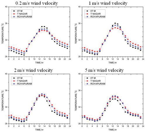
The diurnal temperature profile of the residential site (Royapuram), for the four different velocity conditions, was found to be 31.5, 31.4, 31.2, and 31.1ºC, respectively. The increase in day average temperature compared with background site for the heat load was as follows: 0.35, 0.57, 0.59, and 0.53ºC, respectively. The maximum temperature of 35.5ºC was reported at 2 p.m. (in the afternoon) at 1 m/sec wind velocity condition.

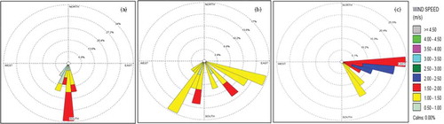
It was found that monitored ambient air temperature was relatively higher than the model day average temperature. The reason was that the vehicular emissions and other anthropogenic heat sources contribute CO₂ emissions, which in turn increase temperature. The limitation of the present Envi-Met model is that it will not consider any anthropogenic heat source in the model simulations. This will result in a rise of local potential temperature due to change in land use. From the results, the highest temperature reached is during low wind conditions (stagnation) at the background site. The correlation between monitoring and modeled diurnal variations of temperature profiles showed good agreement, that is, R² = 0.95 for the background site, R² = 0.947 for the commercial site 0.974, and R² = 0.934 for the residential site. The correlation between the simulated and measured temperature profiles was found to be lower at residential and background sites. At background site, the model showed underprediction of temperature due to surface–air interactions—that is, the air velocity was very low due to the dense forest area. At the residential site, the model showed overprediction because of the model was not accounting for the interactions with the sea breeze that occurs at the study area. The residential study site is located near the seacoast and is significantly (Figure 1) affected by the sea breeze coming from southeasterly directions (see Figure 4).

Figure 4. Wind rose diagrams of the selected sites for monitoring period.

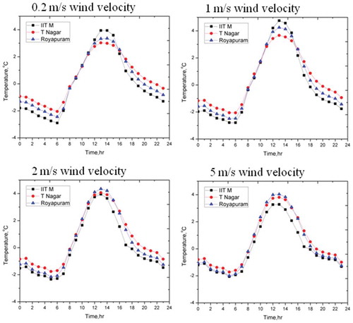
The simulated results also revealed that higher wind speed lowers the UHI intensity during the daytime, whereas lower wind speed increases the UHI intensity during nighttime. The diurnal temperature profiles at Chennai city for the simulated wind speeds (WS), calm condition (WS < 0.2 m/sec), and wind speed of 1 and 2 m/sec indicate an average, and 5 m/sec indicates the maximum wind speed for May–June. Figure 5 presents the 1-hr average temperature profiles for the study regions, and indicates that the highest daytime average temperature was recorded for calm condition (WS < 0.2 m/sec), followed by 1, 2, and minimum at 5 m/sec for three modeled simulations. It is clear from the plot that with the increase in wind velocity, the average temperature at every location is decreasing. This effect is significant for the background site since the specific heat capacity of soil is low and dissipation of heat affects the temperature profiles. For the commercial and residential sites the effect of wind velocity is not significantly affecting the local temperature profile due to poor dissipation conditions with high SVF at these areas. It can be concluded that for the residential site UHI intensity variations were not significant because the percentage of land use change in this region is not affecting the local temperature profile. Thus, it is important to limit the land use change in an urban area for sustainable development.

Figure 5. Diurnal variations of temperature profiles for different wind velocities.

The t-test for paired samples was applied for all wind velocity conditions to find the relation between land use and diurnal temperature profiles corresponding to different wind velocities. We consider the null hypothesis that there is no relation between the land use changes on temperature profile at a particular wind velocity, and the alternative hypothesis that there is. The t-statistics value rejected the null hypothesis (Figure 5 and Table 2).

Table 2. Statistical comparison of model results with t-test: (a) background site, (b) commercial site, and (c) residential site.

Velocity	Mean	Standard deviation	SEM	t-Statistic	Mean difference
(a)
0.2 m/sec	31.18	2.22	0.45	—	—
1 m/sec	30.99	2.25	0.45	4.14	0.26
2 m/sec	30.62	2.01	0.42	5.31	0.50
5 m/sec	30.56	1.75	0.35	4.97	0.67
(b)
0.2 m/sec	31.72	1.69	0.34	—	—
1 m/sec	31.68	1.96	0.40	0.54	0.04
2 m/sec	31.46	1.99	0.40	2.50	0.26
5 m/sec	31.18	1.89	0.38	4.84	0.53
(c)
0.2 m/sec	31.53	1.95	0.39	—	—
1 m/sec	31.48	2.25	0.46	0.47	0.04
2 m/sec	31.26	2.20	0.45	2.60	0.26
5 m/sec	31.07	2.04	0.41	4.19	0.45

Note. Significant differences (p < 0.05) compared to the reference wind speed (0.2 m/sec) are printed in boldface.

Relative humidity

Relative humidity (RH) is an important parameter for air pollutant concentrations because it transforms the reactive pollutants and increases the secondary pollutants concentration. For the present model, the humidity initial condition at 2 m height was 84%, and at 2000 m from atmospheric soundings (http://weather.uwyo.edu/upperair/sounding.html) was 1.99 g/kg; a cyclic boundary condition was used for model simulations.

The correlation between monitored and modeled humidity values at 11 m above ground level was examined. It was estimated that the correlation coefficient (R²) of RH values between the monitored and monitoring for three study regions was not significant.

The Envi-Met model for relative humidity calculations has a limitation in estimation. The cyclic boundary condition for humidity calculations and the humidity contribution due to the sea breeze are major limitations for RH estimation. The Envi-Met model will consider the RH values at equilibrium with temperature at each time interval. The moisture content of the surface cover and the evapotranspiration are considered for simulations. Moisture content due to vehicular emissions and other anthropogenic sources are not considered in the model simulations.

Mixing height measurements and calculations

Mixing height is one of the key components modified by surface modification in urban areas. Ryu et al. (2013b) concluded that the atmospheric boundary layer (ABL) height influences the ozone (O₃) concentration in the urban zone during nighttime. NO₂ to NO conversion at nighttime is an important parameter for O₃ concentration. During a lower ABL condition, the destruction of ozone was less, so this is another important parameter for considering the ozone concentrations during nighttime. During the early morning, higher O₃ concentration was observed due to background concentration and lower mixing height. Mixing height calculations were estimated by considering environmental lapse rate (ELR) at 6 a.m. with dry adiabatic lapse rate (DALR) for every hour in a day. It can be seen from Figure 6 that mixing height variation is a function of wind velocity and percentage of land use change. For the background site, maximum mixing height (MH) was about 450 m corresponding to a wind velocity of 5 m/sec, whereas for the commercial site the maximum mixing height (MH) was about 1100 m, and for the residential site, it was 950 m. At the residential site, the lower wind velocities, that is, 0.2, 1, and 2 m/sec, did not affect the MH variations. For the commercial site these variations were found to be significant with increased wind velocity; 2 m/sec wind velocity condition in the commercial site was equivalent to 5 m/sec in terms of mixing height. At the commercial site, after 2 p.m. MH for 2 m/sec was more than for 5 m/sec, indicating that heat dissipation due to convection was more for 5 m/sec velocity. At the commercial site, the variation of mixing height for 0.2 m/sec and 1 m/sec was significantly higher than 200 m. This indicates that the velocity variations were potentially affecting the temperature profile in the commercial zone. At the residential site the maximum MH, happening at 5 m/sec wind velocity condition, reached 1000 m. For remaining velocity conditions the variation in MH was around 600 ± 250 m. Figure 7 shows the comparison between calculated MH and MH determined by the regional meteorological station at Chennai.

Figure 6. Mixing height variations for different wind velocity conditions at study regions.

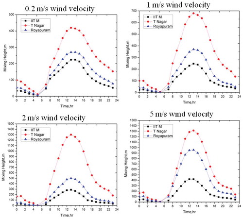
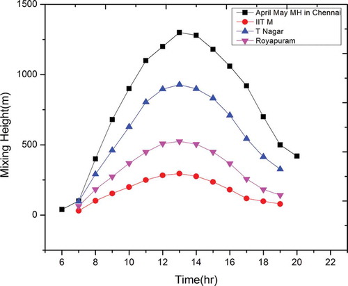
Figure 7. Comparison of mixing heights estimated from the Envi-Met model with IMD mixing height data.

Characterization of UHI effect

Urban heat island (UHI) intensity was modified by different wind velocity conditions. The day average temperature at the background site was 30.8ºC, for the commercial site 31.5ºC, and at the residential site 31.2ºC. With respect to different velocities the diurnal variations of the temperature profiles were significantly different. From Figure 8, it can be observed that at 0.2 m/sec and 5 m/sec wind velocity conditions that UHI intensity is significantly lower than at the other velocity conditions. The impact of the surface covering materials on the UHI intensity is significant after sunset; there is a considerable variation in temperature profiles for different velocity conditions observed from the results.

Figure 8. Characterization of UHI intensity for different velocity conditions.

At the commercial site, 0.2 and 5 m/sec velocities significantly affect the diurnal temperature profiles. However, the wind velocities of 1 and 2 m/sec did not affect the variation in the temperature profile. After sunset, that is, after 18 hr, the variations in local temperature profile showed an interesting phenomenon, namely, a nocturnal heat island effect. It was interesting that the intensity of temperature was increased with the decrease in wind velocity (Oke, 1976). Convective heat transfer from the surface materials was significant in this simulation because of change in land use change, that is, more than 1 degree of temperature increase when wind speed was between 0.2 and 5 m/sec.

The diurnal temperature profiles for different velocity conditions indicated an almost 1 degree temperature rise between 0.2 m/sec and 5 m/sec velocities. The simulation results for the three study regions also indicated the importance of the sky view factor (SVF) on the intensity of temperature rise. The UHI intensity between the background site and the residential site was about 4ºC during the daytime, whereas it was below 3.5ºC for the commercial site. This clearly indicates that the temperature variations during the daytime were influenced by SVF, due to the forced convection process, and during nighttime, by thermophysical properties of the surface materials, due to natural convection.

Ozone (O₃) monitoring

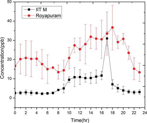
The ambient air quality data collected from the continuous ambient air quality monitoring station (CAAQMS) at residential and background sites were analyzed. Figure 9 indicates the diurnal variation of ozone concentration at the study regions. It can be observed for the plot that the concentration is varying significantly between these two zones, because of variations in primary pollutant emissions. But individual diurnal variations are interesting after sunset; since O₃ formation is a photochemical reaction there will not be any further formation of O₃ after sunset. After 18 hr the O₃ concentration profiles indicated an O₃ dissociation reaction. At early morning, after 1 a.m., the results showed a marginal increment in O₃ concentrations. This indicated that mixing height is playing the major role in formation of secondary pollutants during the nighttime.

Figure 9. Concentration of ozone at selected locations as in Figure 1a and Figure 1c, as averages of measurements during the period.

Conclusion

The air temperature and the height of the mixing layer at the urban background, commercial, and residential sites were simulated using the Envi-Met model. The results showed that the occurrence of highest temperature corresponds to low wind speed and flat mixing layers.

Characterization of UHI intensity with respect to meteorological properties like wind velocity and thermodynamic properties of construction materials has been established. Low wind velocity conditions in the situations leads to high temperature profiles for the all selected study regions. Nocturnal UHI intensity at the background site was not significant with wind velocity variations; for the commercial site and residential site it was 1 ± 0.5ºC for 0.2 to 5 m/sec velocity conditions.

Relative humidity (RH) correlations between measured and model values were not in good agreement. This is because RH calculations in thd Envi-Met model are not accounting for the sea breeze data. With lower mixing height and calm velocity conditions, such as at nighttime, air pollutants are accumulating in the urban environment. This results into deterioration of the air quality through the formation of secondary pollutants (O₃).

Funding

The authors thank the China Section of the Air & Waste Management Association for the generous scholarship they received to cover the cost of page charges, and make the publication of this paper possible.

Additional information

Notes on contributors

Gsnvksn Swamy

Gsnvksn Swamy is a PhD Scholar, Department of Civil Engineering IIT Madras.

S.M. Shiva Nagendra

S.M. Shiva Nagendra is an Associate Professor, Department of Civil Engineering, IIT Madras.

Uwe Schlink

Uwe Schlink is a Senior researcher, Department Urban & Environmental Sociology, Helmholtz Centre for Environmental Research - UFZ.

References

- Jenkin, M.E., and K.C. Clemitshaw. 2000. Ozone and other secondary photochemical pollutants: chemical processes governing their formation in the planetary boundary layer. Atmos. Environ. 34(16):2499–527. doi:10.1016/S1352-2310(99)00478-1
- Li, M., Y. Song, Z. Mao, M. Liu, and X. Huang. 2016. Impacts of thermal circulations induced by urbanization on ozone formation in the Pearl River Delta region, China. Atmos. Environ. 127:382–92. doi:10.1016/j.atmosenv.2015.10.075
- Liao, K.J., E. Tagaris, K. Manomaiphiboon, S.L. Napelenok, J.H. Woo, S. He, and A.G. Russell. 2007. Sensitivities of ozone and fine particulate matter formation to emissions under the impact of potential future climate change. Environ. Sci. Technol. 41(24):8355–61. doi:10.1021/es070998z
- Mahmud, A., M. Tyree, D. Cayan, N. Motallebi, and M.J. Kleeman. 2008. Statistical downscaling of climate change impacts on ozone concentrations in California. J. Geophys. Res. Atmos. 113(D21).
- Memon, R.A., D.Y. Leung, and C.H. Liu. 2009. An investigation of urban heat island intensity (UHII) as an indicator of urban heating. Atmos. Res. 94(3):491–500. doi:10.1016/j.atmosres.2009.07.006
- Mirzaei, P.A. 2015. Recent challenges in the modeling of urban heat island. Sustain. Cities Soc. 19:200–6. doi:10.1016/j.scs.2015.04.001
- Oke, T.R. 1976. The distinction between canopy and boundary‐layer urban heat islands. Atmosphere 14(4):268–77.
- Rizwan, A.M., L.Y. Dennis, and L.I.U. Chunho. 2008. A review on the generation, determination, and mitigation of urban heat island. J. Environ. Sci. 20(1):120–8. doi:10.1016/S1001-0742(08)60019-4
- Ryu, Y.H., J.J. Baik, and S.H. Lee. 2013a. Effects of anthropogenic heat on ozone air quality in a megacity. Atmos. Environ. 80:20–30.
- Ryu, Y.H., J.J. Baik, K.H. Kwak, S. Kim, and N. Moon. 2013b. Impacts of urban land-surface forcing on ozone air quality in the Seoul metropolitan area. Atmos. Chem. Phys. 13(4):2177–94.
- Sarrat, C., A. Lemonsu, V. Masson, and D. Guedalia. 2006. Impact of urban heat island on regional atmospheric pollution. Atmos. Environ. 40(10):1743–58. doi:10.1016/j.atmosenv.2005.11.037
- Tagaris, E., K. Manomaiphiboon, K.J. Liao, L.R. Leung, J.H. Woo, S. He, and G. Russell. 2007. Impacts of global climate change and emissions on regional ozone and fine particulate matter concentrations over the United States. J. Geophys. Res. Atmos. 112(D14).
- Toparlar, Y., B. Blocken, P. Vos, G.J.F. van Heijst, W.D. Janssen, T. van Hooff, and H.J.P. Timmermans. 2015. CFD simulation and validation of urban microclimate: A case study for Bergpolder Zuid, Rotterdam. Build. Environ. 83:79–90. doi:10.1016/j.buildenv.2014.08.004
- Wang, Y., U. Berardi, and H. Akbari. 2015. The urban heat island effect in the city of Toronto. Proc. Eng. 118:137–44. doi:10.1016/j.proeng.2015.08.412
- Wang, Y., U. Berardi, and H. Akbari. 2016. Comparing the effects of urban heat island mitigation strategies for Toronto, Canada. Energy Build. 114:2–19. doi:10.1016/j.enbuild.2015.06.046
- World Health Organization. 2009. Health systems financing: The path to universal coverage. Geneva: World Health Organization.
- Zhao, Z., S.H. Chen, M.J. Kleeman, M. Tyree, and D. Cayan. 2011. The impact of climate change on air quality-related meteorological conditions in California. Part I: Present time simulation analysis. J. Climate 24(13):3344–61. doi:10.1175/2011JCLI3849.1