Statistical analysis of winter ozone exceedances in the Uintah Basin, Utah, USA

ABSTRACT

Because of the confluence of several factors (persistent multiday inversions, petroleum production, and snow cover), the Uintah Basin of eastern Utah, USA, exhibits high concentrations of winter ozone. A regression analysis is presented that successfully predicts daily ozone concentration with a standard error of about 11 ppb. It also predicts with 90% accuracy whether any given day will exceed the National Ambient Air Quality Standard for ozone, 70 ppb. An analysis is introduced for calculating a “pseudo-lapse rate,” a determination of inversion intensity in the absence of sounding data. By combining the model with historical meteorological data, it is possible to make long-range predictions about ozone formation. The odds of observing no exceedance days in any given season are 38%. The odds of only three or fewer exceedance days in any given season are 46%.

Implications: This paper provides an improved understanding of the scientific underpinnings of the winter ozone phenomenon and an ability to make long-range predictions.

Introduction

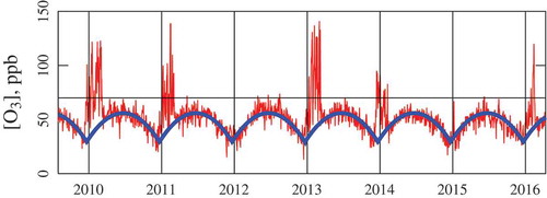
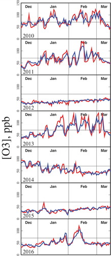
Although tropospheric ozone is typically a summertime urban problem, there are two rural regions in the western USA known to produce significant amounts of wintertime ozone, namely, the Uintah Basin of eastern Utah and the Upper Green River Basin of western Wyoming (Schnell et al., 2009; Martin et al., 2011; Lyman and Shorthill, 2013; Lyman et al., 2013, 2014; Stoeckenius and McNally, 2014; Lyman, 2015, 2016; Lyman and Tran, 2015; Stoeckenius, 2015). The unique factors producing winter ozone in these two basins are summarized in Figure 1. Both basins have a topography that is conducive to persistent multiday thermal inversions during the winter. Both basins are home to an extensive oil and natural gas extraction industry, which generates significant volatile organic compound (VOC) and nitrogen oxide (NO_x) emissions that become trapped near the surface under the inversion layer. Also, high concentrations of winter ozone only occur in the presence of snow cover. Snow significantly enhances the surface albedo, and only in its presence is there adequate actinic flux to form ozone. Furthermore, the ozone system in the Uintah Basin is characterized by the feedback loop represented in Figure 1. The high surface albedo of the snowpack stabilizes inversions, which in turn stabilize the snowpack. Because of a snow-shadow effect, the Uintah Basin tends to receive fewer snowstorms than the Wasatch Front valleys of central and northern Utah (Current Results, 2017). Nevertheless, a single heavy snowstorm can activate the feedback loop, leading to cold temperatures, persistent thermal inversions, a stable snowpack, and numerous exceedances of the ozone National Ambient Air Quality Standard (NAAQS), a day in which the 8-hr running average exceeds 70 ppb, from that moment until springtime. Continuous ozone monitoring has occurred at Ouray, Utah, since mid-2009, as shown in Figure 2 (U.S. Environmental Protection Agency [EPA], 2016). The usual summertime ozone highs are obvious in the data, with occasional summertime exceedances of the NAAQS. However, these are overshadowed by wintertime exceedances during five winters, 2010, 2011, 2013, 2014, and 2016. The two winters 2012 and 2015 had insufficient snow cover to activate the cascade shown in Figure 1. (Throughout this paper, I use a single year number to reference a given winter season, e.g., the winter season extending from December 2011 to March 2012 is denoted Winter 2012.)

Figure 1. Winter ozone requires three ingredients, a snowpack, topography conducive to persistent thermal inversions, and an extensive oil and natural gas extraction industry. The industry is the source of ozone precursors, the inversions keep ozone precursors trapped near the surface, and the albedo of the snowpack ensures adequate actinic flux for the production of ozone. The problem is exacerbated in the Uintah Basin by a feedback loop in which the albedo of the snowpack also stabilizes inversions, which stabilize the snowpack.

Figure 2. Time series of the 8-hr daily ozone maximum at Ouray, Utah, USA, from 31 July 2009 to 11 April 2016. The red trace shows the ozone concentration, whereas the blue trace shows a train of fitted polynomials centered at the summer solstice. The horizontal black line is the NAAQS for ozone, 70 ppb. Each vertical black line indicates 1 January. Five winter seasons out of seven, 2010, 2011, 2013, 2014, and 2016, saw many daily exceedances of the NAAQS.

In this paper, I will present a regression analysis of Uintah Basin winter ozone events. This consists of an effort to predict a dependent variable, i.e., the daily ozone concentration, from the values of a number of independent variables. Such a regression analysis has several uses: (1) We can analyze the relative effect of different independent variables on the formation of ozone. (2) By applying the regression to historical data, we are able to predict the contemporary likelihood that any given winter season will have high ozone, providing in effect a long-range prediction. (3) It can also serve as a tool for short-range forecasting, i.e., if we have reasonable short-term forecasts for each of the independent variables, then the regression provides a short-term forecast of ozone. The first two uses will be explained in this paper, whereas the third is an on-going research effort.

A similar, 3-year study was performed several years ago (Mansfield and Hall, 2013). The current study presents a more extensive analysis, covering 7 years of available data and introducing a more refined technique for defining the independent variable that indicates inversion strength. Furthermore, there has been a decline in global energy prices since the first study, curtailing petroleum production activity in the Uintah Basin, and this study allows us to investigate whether this curtailment has affected ozone formation.

Based on the analysis, I report the following long-range predictions for winter ozone in the Uintah Basin: 38% of years are expected to have no exceedance days of the NAAQS and 46% are expected to be in attainment with three or fewer exceedance days. The odds are 12% that a year will be at least as bad as 2010, the worst winter on record for the total number of exceedance days. The odds are 19% that any three years in succession will produce four or more exceedance days of the NAAQS.

Variables in the regression

Pseudo-lapse rate

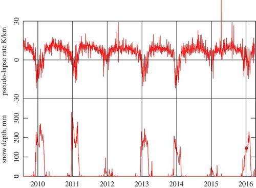
Because of the role of thermal inversions, we anticipate that the lapse rate, defined here as for T temperature and z altitude, should be an important independent variable. However, routine measurements of the lapse rate do not occur in the Uintah Basin. Therefore, I have developed an analysis based on surface temperatures at stations at various altitudes to calculate a variable called the pseudo-lapse rate. I accessed the daily maximum temperature at about 50 stations in the vicinity of the Uintah Basin, as shown in Figure 3, over the seven winter seasons from 2010 to 2016 from the Utah Climate Center (UCC; 2016), an online archive of meteorological data. Figure 4 displays the average in the daily maximum for the dates February 1 through February 14 for which the 8-hr daily maximum ozone concentration at Ouray was either over (filled symbols) or under (open symbols) the value of the NAAQS. The points corresponding to high ozone days separate naturally into two different groups, represented either as filled squares or filled circles. These two groups appear in different regions of the diagram and exhibit positive and negative correlations, respectively, with altitude. Similar diagrams (not shown), prepared for any time period between mid-December to mid-March, display comparable behavior. In any given 2-week time period, the same set of stations having a positive correlation between altitude and average temperature during ozone exceedances are singled out. The logical conclusion is that these stations routinely lie below the inversion layer in the basin. This conclusion is fortified when we see the geographic positions of these stations on the map in Figure 3. All lie within the lower part of the basin, and sites exterior to the basin at comparable altitudes are not included. Therefore, on any given day, we calculate the pseudo-lapse rate from the slope of the least-squares line of maximum daily temperature at these stations against altitude (although because of occasional data gaps, there are days for which not all these stations could be included). Figure 5 shows the time series for the pseudo-lapse rate defined in this way. The most intense inversions are seen in the same years that produce many ozone exceedances.

Figure 3. Map showing the Uintah Basin. White and blue crosses indicate locations of all surface temperature and snow depth stations consulted, whereas the blue crosses give the locations of those stations finally chosen, following an analysis explained in the text, as typically lying under the inversion layer. The town of Ouray is the site of the ozone observations used in this study. The vertical relief extends from about 1350 m above sea level (asl) (green) to about 4125 m asl (blue), with the floor of the basin at about 1400 m asl.

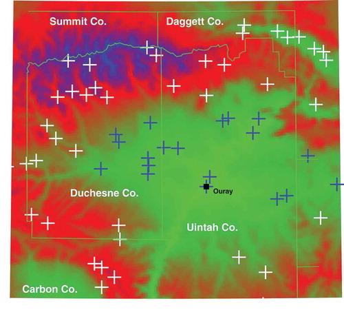
Figure 4. Mean daily maximum in the temperature as a function of altitude at the stations appearing in the map in Figure 3, calculated for the first two weeks of February during each of the winters 2010 to 2016 inclusive. Open and filled symbols represent, respectively, averages taken over days when the 8-hr daily maximum ozone concentration either did or did not exceed 70 ppb. Because they typically lie below the inversion layer, one set of stations, represented with filled squares, behaves differently than another set, represented as filled circles. Lines with indicated slopes are the least-squares fits to filled circles and filled squares, respectively.

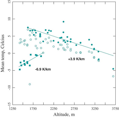
Figure 5. Time-series plots of the pseudo-lapse rate, K/km, and the average snow depth, mm. Vertical lines indicate 1 January.

Snow depth

The Utah Climate Center (2016) also archives historical data on snow depth. Figure 5 shows the basin snow depth averaged over the same stations used to define the pseudo-lapse rate. The average snow depth is greater during the same five winters that produced low lapse rates and high ozone concentrations.

Solar zenith angle

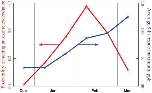
Several lines of analysis indicate that the solar zenith angle is also an important independent variable. Figure 6 shows the probability of experiencing an ozone exceedance at various times throughout the average winter season, computed over the seven years of interest. The probability for an ozone exceedance approaches a maximum of 40% during the first two weeks of February. However, Figure 6 also shows that the average ozone concentration during an exceedance increases steadily during the season. Early in the season, solar radiation is too weak to generate ozone rapidly, whereas late in the season solar radiation is more effective at disrupting inversions but also provides more energy for ozone formation. Therefore, ozone exceedances are more rare in late February and early March, but when they do occur they have higher ozone mixing ratios.

Figure 6. Probability that any given day has an ozone exceedance, and average of the daily 8-hr maximum ozone concentration during an exceedance, at different intervals during the winter.

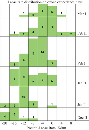
Figure 7 shows a series of histograms, one for each of six different time periods during the winter season. For example, Dec II consists of the dates 15 December to 31 December, whereas Jan I consists of the dates 1 January to 14 January, etc. Each histogram gives the number of days with ozone exceedance occurring during each time period as a function of the pseudo-lapse rate. Intense inversions are required to produce ozone in early winter, but not in late winter. This can also be interpreted as an effect of the solar zenith angle.

Figure 7. Histograms of the distribution in pseudo-lapse rate during ozone exceedance days at different periods throughout the winter. The number of exceedance days represented by each bar is also shown. Early winter ozone requires more intense inversions than late winter ozone.

The effects observed in Figures 6 and 7 might just as well be attributable to the length of daylight as to the solar elevation. However, at any fixed latitude, the two are inextricably linked and a regression analysis would be hard-put to distinguish any effects rising from one or the other. Therefore, I have assumed that the effects of both variables can be subsumed in the regression analysis by either and include only the daily minimum in the solar zenith angle. It is calculated on any given day using the formulas found in Findlayson-Pitts and Pitts (1999).

Basin temperature

The chemical processes leading to ozone formation have temperature-dependent rates, so some temperature dependence may be present. Above we described the linear-least-squares analysis of temperature versus altitude to obtain the pseudo-lapse rate. We use the intercept of the least-squares line at an altitude of 1400 m (near the floor of the basin) to define a daily basin temperature.

Consecutive inversion days

We usually see the ozone concentration increase over the course of a multiday inversion event and attribute this effect to the build-up of ozone precursors. To account for this effect in the regression analysis, we define a variable, “consecutive inversion days” or CIDs, as follows. If on any given date, the pseudo-lapse rate is positive, then let CID for that date equal 0. If the pseudo-lapse rate is negative, then let CID be 1 more than its value on the previous day. According to this definition, CID counts the number of days since the beginning of a multiday inversion event.

Absolute humidity

Ambient H₂O concentrations vary considerably throughout the year. This is important because OH radicals play an important role in ozone production, and the typical production pathway for OH in summer, (Seinfeld and Pandis, 2006), is suppressed in the Uintah Basin in winter. The source of OH radicals in the wintertime Uintah Basin ozone system is still not clear (Edwards et al., 2014; Lyman et al., 2014). In hopes that a regression analysis would provide some clue, we have also included the daily noontime partial pressure of H₂O as an independent variable.

Total petroleum production

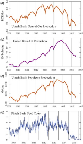
Figure 8 displays time series for the production of oil and natural gas in the Uintah Basin since 2009 (Utah Division of Oil, Gas and Mining [UDOGM], 2016). Because of the recent downturn in global energy prices, both oil and natural gas extraction have declined in the basin since ca. 2014. A regression analysis should indicate whether this recent downturn is reflected in the observed ozone concentration. We have included the total daily tonnage of petroleum production in the Uintah Basin as another independent variable in the regression, under the assumption that petroleum production can act as a surrogate for the emission rate of ozone precursors. Crude oils and natural gases do not all have the same density, and to calculate tonnage, we have assumed the following conversion factors: 19168 tonne/1 billion cubic feet (BCF) natural gas and 0.138 tonne/barrel (bbl) oil.

Figure 8. Uintah basin oil and natural gas activity. Total petroleum production (c) represents the sum of natural gas (a) and oil (b) in tonnage units. The spud count (d) is an estimate of the number of drilling rigs in operation on any given day.

Number of active drilling rigs, or spud rate

The active drilling of new wells has a different emission footprint than production of oil or natural gas from existing wells. Therefore, we also include a daily “spud” rate as an independent variable. (In the jargon of the industry, “spud” represents a new well.) The State of Utah only tabulates the drilling commencement date (UDOGM, 2016). Absent are data on the completion date or the number of active drilling days between commencement and completion. Therefore, to compute a daily spud rate for each well in the state registry, we have assigned 1/15 of a spud to each of days 1 through 15, where day 1 represents the date on which drilling commenced. In this way, the spud rate is an estimate of the number of drilling rigs in operation on any given day. Figure 8 shows the spud rate computed in this way. There is a significant decline near the beginning of 2015.

Ozone concentration

The dependent variable in the regression is the daily maximum in the 8-hr running average at the town of Ouray, Utah (EPA, 2016).

Statistical properties of the variable sets

The regression calculation employed a value of each variable on each day between 15 December to 15 March, inclusive, and for winters 2010 through 2016, including a total of 629 days. (Because of data gaps, a total of 10 days out of 639 are not included.) The complete data set employed is given in the supplementary material. Table 1 tabulates statistical properties of the variables.

Table 1. Statistics on each of the data sets.

Variable	Min	Mean	SD	25th percentile	50th percentile	75th percentile	Max
pseudo-lapse rate, K/km	−22.0	−0.3	7.6	−5.7	1.2	5.9	13.6
Snow depth, mm	0	104	86	10	116	178	305
Consecutive inversion days	0	4.0	8.0	0	0	4	43
Temperature, °C	−18.9	1.0	8.6	−5.2	0.2	7.1	21.5
Zenith angle	42.3°	56.3°	6.7°	50.8°	58.2°	62.6°	63.7°
Petroleum production, Mt/day	0.021	0.026	0.0032	0.024	0.026	0.030	0.031
Spuds	0	1.8	1.1	1.1	2.1	2.7	3.8
H2O partial pressure, mbar	0.7	3.3	1.3	2.3	3.1	4.2	7.5
Ozone, ppb	21	57	24	40	48	68	141

Development of the regression model

Let represent the value of the dependent variable (the ozone concentration) and the value of independent variable j, each on day α. We employ a quadratic regression model, which assumes that the dependent variable can be approximated as follows:

(1)

The regression coefficients A, B_j, and C_jk are obtained by least-squares fitting. We also developed a linear regression model, in which the quadratic coefficients, C_jk, are held at zero. However, using quadratic terms usually allows greater flexibility and versatility, and quadratic terms allow the model to respond to any synergistic effects among the dependent variables. The quadratic regression gives better overall performance and so has been adopted for the current treatment.

For reasons to be explained below, we have considered two versions of the model, Uintah-8, which employs all eight independent variables, and Uintah-5, which employs only five. The two versions are summarized in Table 2. The regression coefficients for the two models are given in the supplementary material.

Table 2. Summary of the models.

UINTAH-5	UINTAH-8
Dependent variable
Ozone concentration^a	Ozone concentration^a
Daily maximum in the 8-hr average at Ouray, UT
Independent variables
1. Pseudo-lapse rate^b	1. Pseudo-lapse rate^b
Calculated from daily maximum surface temperatures
2. Mean snow depth^b	2. Mean snow depth^b
Averaged over many stations
3. Temperature^b	3. Temperature^b
Daily maximum at many stations extrapolated to floor of basin
4. Solar zenith angle^c	4. Solar zenith angle^c
At noontime
5. Consecutive inversion days^b	5. Consecutive inversion days^b
Number of days since initiation of a multiday inversion
	6. Absolute humidity^b
	Partial pressure of H2O
	7. Spud rate^d
	Number of drilling rigs in operation on any one day
	8. Gas and oil production rate^d
	Mt/day

^aEPA (2016).

^bUCC (2016).

^cFindlayson-Pitts and Pitts (1999).

^dUDOGM (2016).

Figure 9 displays the correlation between actual and predicted ozone concentrations for the two models. Pearson’s R² values for the two correlations are 0.75 and 0.78, respectively, and the standard error between actual and predicted ozone concentrations are 12.3 ppb and 11.4 ppb, respectively. Horizontal and vertical lines are drawn at the value of the NAAQS (70 ppb), dividing each plot into quadrants, and the fractions of points falling in each quadrant are shown. A point lying in the lower left quadrant, for example, represents a day that was actually and predicted not to be in exceedance, whereas the upper right includes days that were actually and predicted to be in exceedance. It follows that both versions of the model have a 90% success rate at predicting whether a day will have an ozone exceedance. These findings indicate that Uintah-8 provides only a slight improvement over Uintah-5; inclusion of the three additional independent variables has little effect on model performance. Figure 10 displays time series of actual and predicted ozone concentrations for the seven winter seasons in question. Although the agreement is less than perfect, the model prediction tracks the actual data quite well.

Figure 9. Correlations between measured and predicted ozone. (a) Uintah-5, N = 629, σ = 12.26 ppb, R² = 0.75. (b) Uintah-8, N = 629, σ = 11.36 ppb, R² = 0.78.

Figure 10. Time-series comparisons between actual and predicted ozone concentrations. Red = observation; blue = Uintah-8 prediction.

Other dependent variables, not considered here, that might have improved the performance of the model are the daily ozone column and the daily cloud cover.

The linear regression analysis employed the same five independent variables as Uintah-5. It has a standard error of 14.6 ppb, and although it has an 87% success rate for predicting exceedances, it usually underpredicts ozone concentration for any concentrations above about 90 ppb and below about 40 ppb.

Sensitivity analysis

Figure 11 is presented as a test of the sensitivity of the Uintah-8 model to each independent variable. Eight different curves are shown. Each curve represents the Uintah-8 prediction when the indicated variable is allowed to vary from left to right from the value of its 25th to its 75th percentile (listed in Table 1) while fixing all remaining variables at their 50th percentiles. In this way, we are testing the sensitivity to each variable as it varies over its typical values. The variable plotted along the horizontal axis is

Figure 11. Sensitivity of Uintah-8 to each of its independent variables.

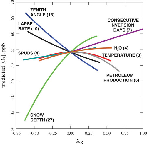
where x_j,₂₅, x_j,₅₀, and x_j,₇₅ are the 25th, 50th, and 75th percentiles of independent variable j. By this definition, all curves cross at the values of their 50th percentile (median). The vertical span of each of the eight curves, shown in parentheses, can be taken as a measure of the sensitivity of the model to each independent variable.

Snow depth has the highest sensitivity at 27 ppb. This of course accords with the observation that ozone exceedances only occur when a snow pack is present. A thin layer of snow is insufficient to cover surface irregularities and vegetation, which helps explain the large value of this sensitivity.

The solar zenith angle, with a sensitivity of 18 ppb, is also seen to be important for predicting ozone concentrations. High angles occur early in the season near the winter solstice and vice versa. The negative trend is therefore consistent with the behavior observed in Figures 6 and 7.

The pseudo-lapse rate has a sensitivity of 10 ppb. Again the negative trend is expected, since a low (negative) lapse rate corresponds to a thermal inversion. In Figure 7, we have seen that weak inversions are capable of producing significant ozone concentrations if the solar angle is low and if a snow pack is present. Therefore, it is not too surprising that the sensitivities of the model to both snow depth and zenith angle are larger than the sensitivity to pseudo-lapse rate.

The number of consecutive inversion days (CIDs) has a sensitivity of 7 ppb, and it trends in the anticipated direction.

Sensitivity to petroleum production is 6 ppb. However, unlike all the variables with higher sensitivities, its downward trend is contrary to our expectation. We do not have a complete understanding of this behavior, but a few observations can be made. As seen in Figure 8, petroleum production was at its lowest for the 2010 and 2016 winters, yet Winter 2010 has had more exceedances than any season on record. That fact alone indicates that petroleum production is probably not a good proxy variable for ozone precursor emissions. Improvements in operating procedures and equipment over the 7-year course of the study suggest the same thing. Finally, with standard error in the model at about 11 ppb, sensitivities around 6 ppb or lower may not have strong statistical significance.

Sensitivity to the spud rate is only 4 ppb, but at least its positive trend accords with our expectation. Again, because of improvements in operating procedures and equipment, the spud rate may not be a good proxy for precursor emissions.

The two remaining variables, H₂O partial pressure and temperature, have the weakest sensitivities. The trend in H₂O is positive, which may be an indication that the O(¹D) → OH reaction, or perhaps other reactions sensitive to H₂O partial pressure, exerts a net positive effect on ozone production. The temperature dependence trends first upwards then downwards, with the maximum almost exactly at 0 °C. This may be a result of a confounding effect: We have already mentioned the significance of the snow pack in winter ozone formation. Perhaps it affects the regression analysis through both the snow depth and the temperature variables. In any case, as already mentioned, sensitivities of 3 or 4 ppb may not be statistically significant.

The relative insensitivity of the Uintah-8 to petroleum production, to the spud rate, and to the H₂O partial pressure explains why Uintah-5 behaves almost as well. We do little damage to the model by omitting those variables. It also reinforces our assertion that such low sensitivities may be an indication of weak statistical significance.

Application to historical data: How often should we expect bad ozone winters?

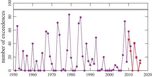
As mentioned above, out of 7 years of data collection, the Uintah Basin has seen five bad ozone winters. One of the main reasons for this study was to make a long-range prediction: How often, on average, can we expect the typical winter to exhibit high ozone? One way of answering this question is to ask how many ozone exceedance days would have occurred in any past year if modern petroleum activity had been in place at the time. Fortunately, data for the five variables used to construct Uintah-5 are available over 66 years into the past. Of course, this application of the model introduces some level of unavoidable uncertainty. Because no ozone data exist prior to 2010, we have no way to independently verify this calculation. Figure 12 displays the number of predicted ozone exceedance days for each winter season since 1951. For comparison, it also displays the actual number of exceedance days for each winter since 2010. The pair of horizontal lines at 90 and 91 days indicate the total length of the winter season as defined in our analysis (all the days between 15 December and 15 March, inclusive, for non-leap and for leap years, respectively). Based on 66 years of predictions, we can make long-range predictions in terms of the odds for several different outcomes. These are given in Table 3. We also see that 1979 would have been a very bad year for ozone, with exceedances occurring almost every day.

Table 3. Predicted odds for various outcomes.

Outcome	Odds
No exceedance days in a season	38%
Annual attainment (three or fewer predicted exceedance days)	46%
A season at least as bad as 2010 (58 or more predicted exceedance days)	12%
Three or more successive years of annual nonattainment	19%

Figure 12. Predictions by Uintah-5 over the past 66 years of the number of exceedance days per year under the assumption that each year had modern petroleum production. Mauve = prediction; red = actual number of exceedance days.

Summary and conclusions

I have presented a successful regression analysis of the winter ozone phenomenon in the Uintah Basin of eastern Utah. Two separate models were considered, Uintah-5 and Uintah-8, with different sets of independent variables as summarized in Table 2. Uintah-8 provides only marginally superior behavior (standard errors of 12.3 ppb and 11.4 ppb in the predicted ozone concentration, respectively; Pearson’s R² values of 0.75 and 0.78, respectively; both models show 90% accuracy at predicting whether a given day will exceed the NAAQS). Both models represent the observed ozone concentrations quite well (Figure 10).

Model sensitivity is strongest for snow depth, solar zenith angle, and the pseudo-lapse rate. The main reason that the two models give comparable results is that they both include these important independent variables and because variables omitted from Uintah-5 prove to be unimportant.

Model sensitivity to petroleum production data is not strong. This is surprising, because we know that ozone precursor emissions by the industry are driving the ozone system and that the level of petroleum activity has been very variable over the course of the study. Perhaps this is because production data are not good proxies for emissions. Over the course of the 7 years of ozone data collection, a number of pollution controls have been adopted (low-bleed pneumatic pumps, emissions controls on storage tanks, green completions, etc.), at least on newer equipment. Therefore, the industry should be able to produce the same amounts of oil or natural gas with fewer ozone precursor emissions.

Another important innovation in this paper is a technique for determining the severity of inversions in the absence of sounding data. The analysis in Figure 4 lets us conclusively identify meteorological stations that lie below the inversion layer, whereas surface temperature measurements at these stations allow us to calculate a “pseudo-lapse rate.”

Of course, Figure 12 does not present actual observational data. Rather, it gives our best estimate, based on the regression formula, for the amount of ozone that would have formed given the meteorological conditions present on any given day since 1951 and assuming that modern ozone precursor emissions were also present. Therefore, it lets us predict the likelihood than any given winter will produce ozone.

Acknowledgment

The author expresses his appreciation to his colleagues of the air quality group at the Bingham Research Center, Utah State University Uintah Basin, for their encouragement and support of this research.

Supplemental data

Supplemental data for this paper can be accessed on the publisher’s website.

Funding

Funding was provided by the Uintah Impact Mitigation Special Services District and the Bureau of Land Management.

Additional information

Funding

Funding was provided by the Uintah Impact Mitigation Special Services District and the Bureau of Land Management.

Notes on contributors

Marc L. Mansfield

Marc L. Mansfield is a research professor at the Department of Chemistry and Biochemistry, Bingham Research Center, Utah State University Uintah Basin, Vernal, UT, USA.

References

- Current Results. 2017. Weather and Science Facts. https://www.currentresults.com/Weather/Utah/annual-snowfall.php ( accessed January 2017).
- Edwards, P.M., S.S. Brown, J.M. Roberts, R. Ahmadov, R.M. Banta, J. A. deGouw, W.P. Dubé, R.A. Field, J.H. Flynn, J.B. Gilman, M. Graus, D. Helmig, A. Koss, A.O. Langord, B.L. Lefer, B.M. Lerner, R. Li, S.-M. Li, S.A. McKeen, S.M. Murphy, D.D. Parish, C.J. Senff, J. Soltis, J. Stutz, C. Sweeney, C.R. Thompson, M.K. Trainer, C. Tsai, P.R. Veres, R.A. Washenfelder, C. Warneke, R.J. Wild, C.J. Young, B. Yuan, and R. Zamora. 2014. High winter ozone pollution from carbonyl photolysis in an oil and gas basin. Nature 514:351–4. doi: 10.1038/nature13767.
- Findlayson-Pitts, B.J., and J.N. Pitts Jr. 1999. Chemistry of the Upper and Lower Atmosphere. San Diego, CA: Academic Press.
- Lyman, S. 2015. Final Report: 2014–15 Uintah Basin Winter Ozone Study. http://binghamresearch.usu.edu/files/UBOS_2015_FinalReport.pdf ( accessed January 2017).
- Lyman, S. 2016. Final Report: 2015–16 Uintah Basin Winter Ozone Study. http://binghamresearch.usu.edu/files/UBOS_2016_FinalReport.pdf ( accessed January 2017).
- Lyman, S., M. Mansfield, and H. Shorthill, 2013. Final Report: 2013 Uintah Basin Winter Ozone & Air Quality Study. http://binghamresearch.usu.edu/files/2013%20final%20report%20uimssd%20R.pdf ( accessed January 2017).
- Lyman, S., and H. Shorthill, 2013. Final Report: 2012 Uintah Basin Winter Ozone & Air Quality Study. http://binghamresearch.usu.edu/files/ubos_2011-12_final_report.pdf ( accessed January 2017).
- Lyman, S., H. Shorthill, M. Mansfield, H. Tran, and T. Tran, 2014. Final Report: 2013–14 Uintah Basin Winter Ozone Study. http://binghamresearch.usu.edu/files/UBOS_2014_FinalReport_.pdf ( accessed January 2017).
- Lyman, S., and T. Tran. 2015. Inversion structure and winter ozone distribution in the Uintah Basin, Utah, USA. Atmos. Environ. 123:156–65. doi: 10.1016/j.atmosenv.2015.10.067
- Mansfield, M.L., and C. F. Hall. 2013. Statistical analysis of winter ozone events. Air Qual. Atmos. Health 6:687–99.
- Martin, R., K. Moore, M. Mansfield, S. Hill, K. Harper, and H. Shorthill. 2011. Final Report: Uinta Basin Winter Ozone and Air Quality Study, December 2010–March 2011. http://binghamresearch.usu.edu/files/edl_2010-11_report_ozone_final.pdf ( accessed January 2017).
- Schnell, R.C., S.J. Oltmans, R.R. Neely, M.S. Endres, J.V. Molenar, and A.B. White. 2009. Rapid photochemical production of ozone at high concentrations in a rural site during winter. Nat. Geosci. 2:120–2.
- Seinfeld, J.H., and S.N. Pandis. 2006. Atmospheric Chemistry and Physics, 2nd ed. Hoboken, NJ: John Wiley & Sons.
- Stoeckenius, T. 2015. Final Report: 2014 Uinta Basin Winter Ozone Study. http://www.deq.utah.gov/locations/U/uintahbasin/ozone/docs/2015/02Feb/UBWOS_2014_Final.pdf ( accessed January 2017).
- Stoeckenius, T., and D. McNally. 2014. Final Report: 2013 Uinta Basin Winter Ozone Study. http://www.deq.utah.gov/locations/U/uintahbasin/ozone/strategies/studies/UBOS-2013.htm ( accessed January 2017).
- U.S. Environmental Protection Agency. 2016. Air Data. http://aqsdr1.epa.gov/aqsweb/aqstmp/airdata/download_files.html ( accessed June 2016).
- Utah Climate Center. 2016. Climate Database Server. Utah Climate Center web site. https://climate.usurf.usu.edu/( accessed January 2017).
- Utah Division of Oil, Gas and Mining. 2016. LiveData Search. http://oilgas.ogm.utah.gov/( accessed December 2016).