Marginal abatement cost curve for nitrogen oxides incorporating controls, renewable electricity, energy efficiency, and fuel switching

ABSTRACT

A marginal abatement cost curve (MACC) traces out the relationship between the quantity of pollution abated and the marginal cost of abating each additional unit. In the context of air quality management, MACCs are typically developed by sorting control technologies by their relative cost-effectiveness. Other potentially important abatement measures such as renewable electricity, energy efficiency, and fuel switching (RE/EE/FS) are often not incorporated into MACCs, as it is difficult to quantify their costs and abatement potential. In this paper, a U.S. energy system model is used to develop a MACC for nitrogen oxides (NO_x) that incorporates both traditional controls and these additional measures. The MACC is decomposed by sector, and the relative cost-effectiveness of RE/EE/FS and traditional controls are compared. RE/EE/FS are shown to have the potential to increase emission reductions beyond what is possible when applying traditional controls alone. Furthermore, a portion of RE/EE/FS appear to be cost-competitive with traditional controls.

Implications: Renewable electricity, energy efficiency, and fuel switching can be cost-competitive with traditional air pollutant controls for abating air pollutant emissions. The application of renewable electricity, energy efficiency, and fuel switching is also shown to have the potential to increase emission reductions beyond what is possible when applying traditional controls alone.

Introduction

Nitrogen oxides (NO_x) are emitted when fossil fuels are combusted. In the atmosphere, NO_x reacts with volatile organic compounds (VOCs) to produce tropospheric ozone (O₃), a component of photochemical smog. Strategies for reducing O₃ typically focus on modifying combustion processes or placing emission control devices on power plants, other industrial sources, and vehicles. However, additional measures for reducing emissions may also need to be explored, for example, when traditional controls have been fully deployed. Nontraditional abatement measures such as renewable electricity, energy efficiency, and fuel switching (RE/EE/FS) have the potential to increase emission reductions considerably beyond what is possible when applying traditional controls alone.

Although energy system models have not typically been used to develop air quality management strategies, these models have the potential to facilitate examination of nontraditional abatement measures such as RE/EE/FS. We applied one such model to develop national and regional marginal abatement cost curves (MACCs) for NO_x that incorporate both traditional air pollutant controls and RE/EE/FS. We decomposed the curves to examine the emission reduction potential and the relative cost-effectiveness of RE/EE/FS. The regional MACCs provide insights regarding important geographic differences in abatement capacity. Although this paper is focused on the development of MACCs for NO_x, the approach could readily be extended to other pollutants, including other precursors to O₃ formation such as VOCs.

The resulting illustrative MACCs are specific to the underlying data and assumptions, as well as to our hypothetical implementation of future NO_x reduction goals. In the Summary section, we describe a number of caveats and discuss our future research directions to develop MACCs that could be used in support of regional and national air quality decision-making.

Background

A MACC, which depicts the relationship between pollution abatement and cost, is often represented as a piece-wise linear curve or as a step curve on an x-y plot. In the context of air quality management, the x-axis typically represents tons of emissions reduced, whereas the y-axis represents the cost of reducing the last ton of emissions at that level of overall abatement. Moving from left to right on the x-axis yields increasing emission reductions at higher marginal costs, typically producing a monotonically increasing relationship.

Morris et al. (2012) characterize two classes of applications of MACCs. The first is as a pedagogic tool that simplifies the complexities of abatement into a representation that can readily be understood and evaluated by decision makers. The second use is as a reduced-form characterization of abatement control that can be incorporated into another model. In the pedagogic context, a MACC has a number of uses in air quality management. Integrating under the curve to a particular reduction level yields an estimate of the associated abatement cost. Furthermore, the MACC can be used to quantify the amount of abatement that is economically achievable, approximate how much abatement would occur at a given tax on emissions, estimate the permit price under a cap-and-trade program, and understand the relative cost-effectiveness of various mitigation options (Kesicki and Strachan, 2011). Within a cost-benefit analysis framework, MACCs can be used to identify the economically efficient level of abatement at which marginal costs equal marginal benefits (U.S. Environmental Protection Agency [EPA], 2014a).

The MACC concept was formally introduced into the literature in 1982, where it was used to examine cost savings associated with energy efficiency (Meier et al., 1982). Since then, MACCs have been applied to a wide range of efforts. Several of the more widely discussed examples include those of Jackson (1991) and McKinsey and Company (Creyts et al., 2007; McKinsey and Company, 2010), both of which characterized abatement costs for a range of greenhouse gas abatement measures. The MACC concept was formally introduced to air quality management literature by Rentz et al. (1994), who used an energy system optimization model to develop MACCs for sulfur dioxide (SO₂).

Understanding how a MACC was created is important in interpreting its results and understanding its applicability (Kesicki and Strachan, 2011). Most MACCs can be classified as having been developed via either top-down or bottom-up methods, or as being non-model-derived or model-derived (Delarue et al., 2010). Kesicki (2011) presents a lexicon that describes these categories. Non-model-derived MACCS are developed by characterizing the costs and abatement potential of the available measures, then ordering those measures by cost-effectiveness. Note that Kesicki originally referred to non-model-derived MACCs as being “expert-derived.” We propose this new terminology to avoid confusion with expert elicitation methods. Model-derived MACCs are developed by running an economic or energy system model iteratively, applying an incrementally increasing pollutant tax in each iteration. Model-derived approaches are further differentiated by the type of model used. Bottom-up models have a comparatively high level of technological detail about abatement options but have a more simplified representation of economic considerations.

The strengths and limitations of various approaches for developing and using MACCs have received considerable discussion. For example, Stoft (1995) identify drawbacks that include lack of consideration of cross-sector impacts, economic feedbacks, and demand rebounds. Meier et al. (1982) raised the possibility of abatement options not being independent, which could lead to double-counting if not handled. For example, a water heater insulation blanket would not be as effective if a thermostat set-back measure had already been adopted. Thus, if the abatement potential from these two measures is summed independently, the abatement estimate would be unrealistically high. McKinsey and Company (McKinsey and Company, 2010) indicated that considerable emission reductions were possible at a negative cost, precipitating discussion regarding why these reductions had not been adopted already (Murphy and Jaccard, 2011; Taylor, 2012; Levihn, 2016).

Model-derived MACCs address many of these shortcomings. If the underlying model captures cross-sector effects, such as competition for fuel between sectors, the resulting MACCs will incorporate information on those cross-sector effects. Also, model-derived MACCs avoid the problem of double-counting, as occurs in the water heater example above, if the model includes logic that avoids such a result. A disadvantage of model-derived MACCs is that the complexity of the modeled system may complicate tasks such as identifying the specific technological pathway taken by the model or producing a definitive ranking of abatement measures. Instead, insights may be limited to the sectoral level (Kesicki and Strachan, 2011).

Kesicki and Strachan (Kesicki and Strachan, 2011) point out limitations shared by both non-model-based and model-based methods that would lead to divergence of the MACCs from real-world behavior. These limitations include factors such as lack of consideration of nonfinancial costs, market failures and barriers, and path dependencies, as well as unmodeled interactions among geopolitical regions and inherent uncertainty in future policies and technology development. Recent literature delves into these and similar issues (e.g., Klepper and Peterson, 2006; Delarue et al., 2010; Morris et al., 2012; Taylor, 2012; Levihn et al., 2014; Ward, 2014).

There have been a number of recent applications of air pollutant MACCs in the academic literature, including by Reis (2005), Vijay et al. (2010), and Wu et al. (2015), all of whom develop non-model-derived MACCs. MACCs also have been used in practice, such as by the EPA within Regulatory Impact Analyses (RIAs). Examples include the 2008 and 2015 RIAs for the National Ambient Air Quality Standard (NAAQS) for ozone (EPA, 2008, 2015b), in which non-model-derived MACCs were created for abating nitrogen oxides (NO_x). The MACCs primarily consisted of control measures from the Control Strategy Tool (CoST) (EPA, 2014b). CoST includes a comprehensive database of traditional air pollutant controls, such as low-NO_x burners and selective catalytic reduction (SCR) devices, that reduce NO_x emissions (EPA, 2017a). CoST currently contains relatively few options for reducing emissions via fuel switching and does not include measures such as energy efficiency, renewable electricity, or vehicle electrification.

In the research presented here, we explore the utility of bottom-up, model-derived MACCs for air pollutants, focusing on NOx. Although the prior EPA MACCs examined the traditional controls in CoST only, the sector- and region-specific MACCs developed here combine both traditional controls and RE/EE/FS. Thus, this approach incorporates a broader portfolio of pollution abatement measures and successfully quantifies and monetizes the additional reductions that are achievable.

Our empirical approach relies on the EPA MARKet ALlocation (MARKAL) modeling framework. The framework consists of the MARKAL energy system model (Loulou et al., 2004) and the EPAUS9r_2014_v1.5 MARKAL nine-region database (EPA, 2013), which was modified to incorporate representations of traditional NO_x controls. MARKAL is an optimization model that identifies the lowest-cost energy technologies and fuels that meet the specified energy demands and performance constraints over the modeled time period. The database includes current and projected characterizations of U.S. energy demands, renewable and fossil resources, and energy production, transformation, and end-use technologies. The database also includes emission factors for a range of traditional air pollutants. The use of this database within the MARKAL optimization framework permits a detailed examination of the potential RE/EE/FS play in reducing emissions. For a given U.S. energy system scenario, the EPA MARKAL framework produces fuel use, technology penetration, and emission estimates through 2055 at the U.S. Census Division level. For reference, Table 1 lists the MARKAL regions, the corresponding U.S. Census Divisions, and the states within each.

Table 1. List of MARKAL regions and corresponding U.S. Census Divisions and states.

MARKAL region	U.S. Census Division	States
1	New England	CT, ME, MA, NH, RI, VT
2	Middle Atlantic	NY, NJ, PA
3	East North Central	IN, IL, MI, OH, WI
4	West North Central	IA, KS, MN, MO, NE, ND, SD
5	South Atlantic	DE, DC, FL, GA, MD, NC, SC, VA, WV
6	East South Central	AL, KY, MS, TN
7	West South Central	AR, LA, OK, TX
8	Mountain	AZ, CO, ID, NM, MT, UT, NV, WY
9	Pacific	AK, CA, HI, OR, WA

Note. U.S. Postal Service abbreviations are used for states.

The EPA MARKAL Base Case scenario used in this study has been calibrated to approximate the technology assumptions and fuel use estimates of the U.S. Energy Information Administration’s (EIA) 2014 Annual Energy Outlook (U.S. EIA, 2014). In addition, the Base Case incorporates approximations of state-level renewable portfolio standards and air pollution regulations such as the Cross State Air Pollution Rule (EPA, 2011), the Tier 3 mobile source emission standards (EPA, 2014c), and the Clean Power Plan (EPA, 2015a). Emission factors are derived from a number of sources, including the EPA’s WebFIRE (EPA, 2017b), Greenhouse Gas Inventory (EPA, 2012), and the MOtor Vehicle Emission Simulator (MOVES) (EPA, 2010).

Methodology

Data were drawn from CoST to characterize currently available NO_x controls in the industrial, residential, commercial, and off-highway transportation sectors. See the supplemental material for a description of how controls were characterized. These controls were then added to the MARKAL database, complementing the electric sector NO_x controls already represented. Incorporation of controls allows the model to react to the imposition of NO_x emission constraints or per-ton emission taxes with the lowest-cost combination of both controls and RE/EE/FS.

Next, baseline regional NO_x trajectories over the modeling horizon were estimated from the MARKAL Base Case. A maximum traditional control case was also run in which traditional controls were fully deployed, without any explicit measures to adopt RE/EE/FS. Note that some RE/EE/FS may be applied endogenously as the model reacts to the additional cost of control measures. For example, in the maximum traditional control scenario, all coal-fired electricity production was required to use SCR. This requirement would increase the cost of that production, so the model could respond with some amount of fuel switching to other fuels or technologies, such as natural gas combined-cycle turbines.

We then iteratively executed MARKAL, forcing increasingly stringent regional NO_x reduction constraints upon the baseline with each iteration, including traditional controls and RE/EE/FS. These constraints reduced 2035 NO_x emissions from each region, starting at 2.5% from baseline 2035 levels and decreasing in 2.5% increments to a 40% reduction. The constraints were implemented linearly from 2015 to 2035 and held constant after 2035.

Note that to more clearly trace out regional MACCs, we apply a percent reduction constraint to each region rather than a national or regional pollutant tax as described by Kesicki and Strachan (Kesicki and Strachan, 2011). Use of a tax can result in the model making decisions that result in nonmonotonically increasing MACCs. For example, the model may react to a marginal increase in emission tax rate by shifting electricity production from one region to another. Although emission reductions would occur in the aggregate, the regional response would vary by region. Requiring each region to simultaneously meet the same percent reduction target avoids this type of issue and, as a result, produces more easily interpretable regional MACCs.

The year 2035 was selected as the end point for the trajectories, as well as the year for which MACCs are calculated for several reasons: (i) 2035 is at the far end of the range of years for which regulatory impact analyses typically have been conducted by the EPA; (ii) 2035 is far enough into the future that significant technological turnover can occur; and (iii) there is less uncertainty in factors such as population growth, economic growth, and technological development that would be expected in later years such as 2050. Although the emission constraints are tightened over the 2015–2035 period in a linear fashion, representing a gradual flightpath to achieving emission reductions, alternative approaches to designing the constraints are possible.

The spatial resolution at which the emission reduction targets are modeled affects the resulting MACCs. For example, faced with a national reduction target, MARKAL would efficiently allocate the required emission reductions across regions, potentially leading to situations where some regions could even increase emissions as long as the national reduction target is met. Thus, the use of a national constraint may not yield directly applicable regional MACCs. However, by applying regional constraints in developing our MACCs, we are able to develop meaningful region-specific curves that could also be aggregated to the national level.

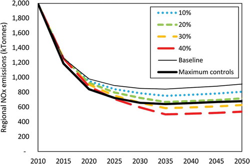
Figure 1 illustrates emission levels in the baseline and under the maximum traditional control scenario in the South Atlantic U.S. Census Division, which is Region 5 in the MARKAL database, as well as several emission reduction constraints. Since the 30% and 40% reduction trajectories are below the maximum control trajectory, they cannot be achieved without nontraditional measures, such as RE/EE/FS.

Figure 1. Example of NO_x emissions for baseline and maximum traditional controls scenarios, as well as incrementally more stringent regional NO_x constraints for Region 5, the South Atlantic.

In total, 22 MARKAL runs were conducted, including the baseline, maximum traditional control scenario, and alternative regional NO_x trajectory constraints. For each run, recorded outputs include technology penetrations, fuel use, application of controls, sectoral emissions, and marginal NO_x abatement costs.

Results and discussion

Figure 2 depicts the resulting MACC for NO_x at the national level. Marginal costs for this MACC and others presented in this paper are in 2005 U.S. dollars. For each reduction scenario, the marginal abatement cost represents the weighted average of the marginal abatement costs across the nine MARKAL regions. This MACC includes both traditional controls and RE/EE/FS. Base Case NO_x emissions in 2035 are approximately 6000 ktonnes, so 2000 ktonnes would constitute an emission reduction of approximately one-third. Note that Base Case NO_x emissions in 2035 are projected to be substantially lower than recent levels (about 14,000 ktonnes in 2011) because of the suite of requirements and technological trends included in the Base Case, such as existing air pollutant regulations on stationary and mobile sources that are expected to lead to substantial emission reductions in future years. These substantial reductions already in the Base Case highlight why obtaining further NO_x reductions may be challenging in the future (e.g., since traditional controls have already been accounted for) and may require alternative mitigation approaches such as RE/EE/FS to reduce NO_x significantly further.

Figure 2. National MACC for NO_x for 2035.

Comparing the results shown in the MACC with those of the maximum traditional control scenario illustrates that inclusion of RE/EE/FS expands the amount of emissions that can be abated and that it does so in a cost-effective manner. For example, the maximum traditional control scenario reduces national NO_x emissions in 2035 by 1240 ktonnes at a marginal cost of $10,300 per tonne. At a similar marginal cost, the MACC suggests 1500 ktonnes of abatement is achievable.

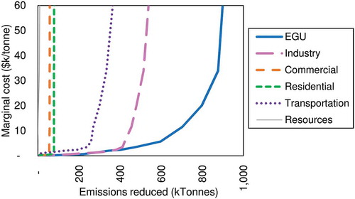
In Figure 3, we decompose this MACC into its sectoral contributions. These results indicate that reductions are achievable from all sectors at marginal costs below $60k/tonne. The sectors that provide the greatest reduction opportunities are the electric generating unit (EGU), industrial, and transportation sectors. In these sectors, the marginal abatement costs appear to increase rapidly beyond approximately $5k/tonne, although the rate of increase is more gradual for the EGU sector. Meanwhile, reductions from the residential and commercial sectors provide relatively little abatement potential, although their abatement opportunities are comparatively inexpensive. Very little reduction potential is associated with the resource sector, which primarily consists of fossil fuel extraction activities.

Figure 3. National, sectoral MACCs for NO_x for 2035.

Figure 4 decomposes the MACC into its constituent curves for traditional controls and RE/EE/FS. These components can be separated, since the results (marginal costs and emission reductions) for traditional control reductions and total reductions are reported by MARKAL. Explicitly disaggregating the resulting RE/EE/FS curve into its individual RE, EE, and FS components is not readily accomplished, since there are considerable interactions among these components. For example, a switch to a more energy-efficient end-use technology may also involve fuel switching. We do not attempt this disaggregation, although it may be worth exploring in future work.

Figure 4. National MACC for NO_x for 2035, as well as MACCs for reductions attributed to traditional controls and RE/EE/FS.

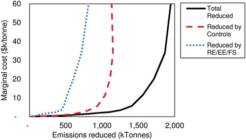
These results point to an important finding: RE/EE/FS were able to produce approximately 30–40% reduction beyond traditional controls, up to $60k/tonne. The share of reductions attributable to RE/EE/FS increased further at higher levels of abatement. Although the overall MACC is monotonically increasing, as expected, the curve formed from the underlying contribution of traditional controls to the MACC begins to double back as overall emission reductions approach 2000 ktonnes and reductions from traditional controls approach approximately 1200 ktonnes.

Note that $60k/tonne is assumed to be the marginal cost above which controls are considered too expensive. This value is more than 10 times greater than the cost of SCR. In the real world, many factors would factor into the decision of what marginal cost is considered too high, and this value may be greater than or less than $60k/tonne.

Figures 5 and 6 are presented to explain this outcome further. Figure 5 shows the electric sector MACC and its components, inverted so that we can more readily visualize how NO_x reductions respond to increasing marginal costs.

Figure 5. National electric-sector MACC for NO_x for 2035, oriented with marginal cost on the x-axis.

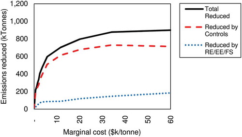
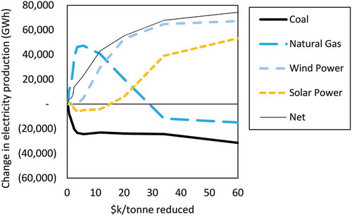
Figure 6. Change in electricity production by fuel in 2035 as a function of marginal cost. Electricity production by fuels or technologies not shown on the graphic (e.g., oil, biomass, nuclear, and hydropower) did not change.

Figure 5 illustrates that in the electric sector, a large majority of the traditional controls are applied at a marginal cost of $10k/tonne or less. The remaining control-related reductions are incrementally applied through costs up to about $35k/tonne. However, above this marginal cost, the control-related reductions begin to diminish gradually as marginal costs increase. Thus, the national-level supply of abatement from control-related reductions is backward bending for the EGU sector, and RE/EE/FS contribute an increasing share of NO_x reductions as overall NO_x emission reductions increase.

Figure 6 shows how electricity production by fuel type responds to increasing marginal costs, highlighting some of the underlying drivers affecting the aggregated results in Figure 5. For reference, total Base Case electricity production in 2035 is approximately 33,000 PJ, with one-third from coal and one-third from natural gas.

As the marginal costs increase, MARKAL transitions away from coal toward less NO_x-intensive fuels. A portion of the traditional controls for coal is thus no longer applicable, since the model has shifted from coal to other fuels. Thus, fuel switching is responsible for the back-bending behavior of the control curve. This result illustrates how our model-based approach for deriving MACCs can avoid the issue of double-counting pollutant controls.

Figure 6 depicts this behavior. At marginal costs less than $5k/tonne, coal is replaced with natural gas. However, the role of gas diminishes as marginal costs increase beyond $5k/tonne. Starting at $28k/tonne, natural gas use is lower than in the Base Case. Output from wind is increasing at marginals greater than $5k/tonne, but very little additional capacity is added after $35k/tonne.

Although reliance on solar power decreases at marginal costs up to $15k/tonne, it then increases rapidly at higher marginal costs. This result, which is driven by electric sector changes in the South Atlantic Census Division, illustrates one of the insights that can be provided with MARKAL. Since coal is a base-load technology that generates electricity day and night, it is not easily replaced with solar photovoltaic (PV) generation that generates electricity only during the day. Instead, in the South Atlantic, coal is replaced by natural gas, which has more flexibility than coal or solar in terms of seasonal and time-of-day operations. Once solar enters the solution at higher marginal costs, however, it does so by replacing natural gas. A portion of the remaining gas capacity is then able to increase output at night when solar power is not producing electricity. Coal would not be able to ramp up and down economically in a similar fashion.

Figure 6 also indicates that end-use fuel switching is occurring. We did not evaluate which end uses were undergoing fuel switching, but available options include vehicle electrification and greater adoption of electric heat pumps for space conditioning. With greater restrictions on NO_x emissions, and evaluating how to most cost-effectively meet those targets from a system perspective, MARKAL opts to transition some end uses from fossil fuels to electricity, increasing electricity production. Figure 6 is also notably based upon what does not appear. For example, MARKAL does not find introduction of additional nuclear power plants to be a cost-effective means of reducing NO_x in the scenarios we examine here. Similarly, biomass does not play a major role in these results, at least at the national scale.

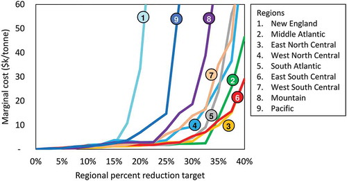
Figure 7 presents the regional MACCs as a function of the regional percent reduction of NO_x. These results indicate that the MACC can be very different from one region to another. Regions with relatively high utilization of coal in electricity production, such as the Middle Atlantic (2), East North Central (3), and East South Central (6), have more reduction potential, as indicated by their MACCs being lower and shifted to the right. In contrast, New England (1) and the Pacific (9) rely more on natural gas and other technologies. Their reduction potentials from controls and from fuel switching are thus more limited.

Figure 7. Regional MACCs for NO_x in 2035.

In Figure 8, we examine the relative role of RE/EE/FS in each region. The percentages of regional reductions achieved by RE/EE/FS are shown as a function of the 2035 NO_x reduction target. For example, the combination of a 40% regional reduction target and 20% reduction from RE/EE/FS indicates that half the 40% reduction target is being met by RE/EE/FS. The last regional target level at which the regional marginal cost for NO_x reduction is less than $60k/tonne is indicated by a marker on each series on the figure.

Figure 8. RE/EE/FS portion of regional MACCs in 2035 (percent of NO_x emissions reduced; e.g., the combination of a 40% regional reduction target and 20% reduction from RE/EE/FS would indicate that half the reduction target was met by RE/EE/FS). The markers along each series indicate the last reduction target at which the marginal was less than $60k/tonne.

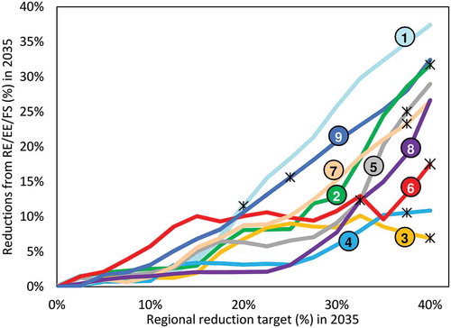
All regions are shown to have the potential to meet some fraction of the regional reduction target via RE/EE/FS. For a 40% regional reduction target, this potential varied from approximately one-sixth in the East North Central region (3) to nearly all in New England (1). The results also show considerable regional variability in both RE/EE/FS potential and cost-effectiveness. Regions with high percentages of Base Case 2035 electricity generation from coal (e.g., West North Central [4]: 52%; Mountain [8]: 42%) tend to have a relatively low portion of reduction achieved by RE/EE/FS, at least until traditional controls have been fully deployed. In contrast, the New England (1) and Pacific (9) regions generate a much lower fraction of electricity from coal and thus must turn to RE/EE/FS. With limited traditional control opportunities, their mitigation costs are higher. For example, in the New England (1) and Pacific (9) regions, marginal costs begin to exceed $60k/tonne at 20% and 25% NO_x reduction targets, respectively. Other regions can achieve 37.5% or 40% before marginal abatement costs exceed this value.

Summary

We demonstrate the use of the EPA MARKAL energy system framework in developing national and regional MACCs for NO_x that incorporate both traditional controls and nontraditional measures, such as renewable electricity, energy efficiency, and fuel switching (RE/EE/FS). This application adds to the academic literature in energy and environmental modeling by presenting an approach to estimating MACCs that simultaneously accounts for traditional controls and RE/EE/FS. From an air quality management perspective, the study results are of interest because we quantify the region-level NO_x emission reductions achievable by traditional controls and RE/EE/FS and the costs associated with these reductions, illustrating that a portion of RE/EE/FS appear to be cost-competitive with traditional controls.

These results indicate that MACCs built from traditional controls alone underestimate abatement supply and overestimate the cost compared with the reductions that could be achieved if a more complete portfolio of options were to be considered. The results also point to the utility of considering traditional controls and alternative measures in a single decision-analysis framework and indicate that energy system models may be good tools for this purpose. In particular, the result of a backward-bending relationship between emission reductions from traditional controls and marginal cost illustrates how MARKAL can capture complexities such as the reduced abatement potential from coal-fired power plants in modeling scenarios where these technologies are replaced by other technologies or fuels.

Another observation is that some specific RE/EE/FS are not implemented in model solutions at marginal costs of less than $60k/tonne, which would be expensive for NO_x reductions. However, many of these RE/EE/FS can provide multipollutant benefits. As a result, multipollutant reduction strategies may lead to a higher level of penetration of these technologies than strategies that focus on single pollutants only. The energy system modeling approach described here could be extended to evaluate a multipollutant approach.

An important consideration we demonstrate is that the potential role of RE/EE/FS in reducing NO_x differs by region of the country. Further disaggregation of the regional results by sectoral fuel and technology choices may help in identifying the most cost-effective strategies for introducing specific RE/EE/FS at the regional level.

In discussing the methodology, we previously highlighted that a MACC developed using a national emission constraint may not be directly applicable to a particular region, since the model would allocate abatement across regions based on cost-effectiveness. A similar consideration should be taken into account when evaluating the utility of a regional MACC for state-level decisions. The MACC could provide some guidance regarding regional abatement potential and cost. Implicit in the MARKAL regional result, however, is that state-level results would vary, also influenced by factors such as differences in baseline state-level technology capacities and by renewable potential that are not captured within a regional model.

Many caveats should be noted. The MACCs presented here are intended to be illustrative. Their integration into an optimization or planning model to represent abatement options may not be appropriate if that model also includes traditional controls or RE/EE/FS. Furthermore, the MACCs are specific to the assumptions made during this exercise. For example, we use technology performance assumptions primarily derived from the Annual Energy Outlook (AEO) 2014 Reference Case scenario. Alternative assumptions about technology availability and performance, as well as alternative assumptions about impacts of policies in the baseline, would influence results in the Base Case and the NO_x-constrained scenarios.

Another consideration is that the MACCs presented in this paper focus on 2035 alone. Analysis of an alternative future year would yield different MACCs. A challenge in an analysis spanning multiple decades is how to consider time-dependent results. In other words, although we focus on results in 2035, these results depend upon modeled decisions in previous periods as well as how decisions in 2035 influence modeled decisions in later periods. Similarly, the iterative approach used to develop the curves assumed a linear transition to the ultimate NO_x reduction targets. Alternative assumptions, such as nonlinear trajectories, would undoubtedly affect the resulting MACCs.

The curves developed in this study are for only one possible realization of the future. There are deep uncertainties regarding many of the drivers of future emissions, including future population growth and migration, economic growth and transformation, technology development, behavioral and land use choices, and any additional future policies. One approach for addressing these uncertainties would be to calculate MACCs for wide-ranging scenarios of the future, exploring commonalities and differences in the possible roles for traditional controls and RE/EE/FS.

Disclaimer

Although this paper has been reviewed and cleared for publication by the EPA, the views expressed here are those of the authors and do not necessarily represent the official views or policies of the agency. Mention of software, models, and organizations does not constitute an endorsement.

Acknowledgment

A number of additional people contributed to this work. Motivation to explore measures beyond traditional controls originated through discussions among the authors and Julia Gamas and Darryl Weatherhead of the EPA’s Office of Air Quality Planning and Standards. Alison Eyth and David Misenheimer provided the emission inventory and control data, respectively, used to develop the characterization of traditional controls in MARKAL. Development of the EPAUS9r MARKAL database has been a collaborative effort within the EPA’s Office of Research and Development. Those with contributions most germane to this study include Carol Lenox, Rebecca Dodder, Ozge Kaplan, and William Yelverton, although there have been a host of additional contributors, including former EPA employees, postdoctoral fellows, student interns, and contractors.

Supplemental data

Supplemental data for this article can be accessed on the publisher’s Web site.

Additional information

Notes on contributors

Daniel H. Loughlin

Daniel H. Loughlin, Ph.D., is a senior physical scientist with the EPA Office of Research and Development.

Alexander J. Macpherson

Alexander J. Macpherson, Ph.D., is a senior economist with the EPA Office of Air Quality Planning and Standards.

Katherine R. Kaufman

Katherine R. Kaufman is a policy analyst with the EPA Office of Air Quality Planning and Standards.

Brian N. Keaveny

Brian N. Keaveny is an economist with the EPA Office of Air Quality Planning and Standards.

References

- Creyts, J., A. Derkach, S. Nyquist, K. Ostrowski, and J. Stephenson. 2007. Reducing U.S. Greenhouse Gas Emissions: How Much at What Cost? U.S. Greenhouse Gas Abatement Mapping Initiative, Executive Report. New York: McKinsey & Company.
- Delarue, E.D., Ellerman, A.D., and W.D. D’Haeseleer. 2010. Robust MACCs? The topography of abatement by fuel switching in the European power sector. Energy 35:1465–75. doi: 10.1016/j.energy.2009.12.003.
- Jackson, T. 1991. Least-cost greenhouse planning supply curves for global warming abatement. Energy Policy 19:35–46. doi: 10.1016/0301-4215(91)90075-Y.
- Kesicki, F. 2011. Marginal Abatement Curves for Policy Making—Expert-Based vs. Model-Derived Curves. Report—UCL Energy Institute. London: University College London.
- Kesicki, F., and N. Strachan. 2011. Marginal abatement cost (MAC) curves: Confronting theory and practice. Environ. Sci. Policy 14:1195–204. doi: 10.1016/j.envsci.2011.08.004.
- Klepper, G., and S. Peterson. 2006. Marginal abatement cost curves in general equilibrium: The influence of world energy prices. Resour. Energy Econ. 28:1–23. doi: 10.1016/j.reseneeco.2005.04.001.
- Levihn, F. 2016. On the problem of optimizing through least cost per unit, when costs are negative: Implications for cost curves and the definition of economic efficiency. Energy 114:1155–63. doi: 10.1016/j.energy.2016.08.089.
- Levihn, F., Nuur, C., and S. Laestadius. 2014. Marginal abatement cost curves and abatement strategies: Taking option interdependency and investments unrelated to climate change into account. Energy 76:336–44. doi: 10.1016/j.energy.2014.08.025.
- Loulou, R., Goldstein, G., and K. Noble. 2004. Documentation for the MARKAL Family of Models. Paris: Energy Technology Perspectives Programme. http://unfccc.int/resource/cd_roms/na1/mitigation/Module_5/Module_5_1/b_tools/MARKAL/MARKAL_Manual.pdf (accessed January 31, 2017).
- McKinsey and Company. 2010. Climate Change Special Initiative—Greenhouse Gas Abatement Curves. New York: McKinsey and Company.
- Meier, A., Rosenfeld, A.H., and J. Wright. 1982. Supply curves of conserved energy for California’s residential sector. Energy 7:347–58.
- Morris, J., Patlsev, S., and J. Reilly. 2012. Marginal abatement costs and marginal welfare costs for greenhouse gas emissions reductions: Results from the EPPA model. J. Environ. Model. Assess. 17:325–36. doi: 10.1007/s10666-011-9298-7.
- Murphy, R., and M. Jaccard. 2011. Energy efficiency and the cost of GHG abatement: A comparison of bottom-up and hybrid models for the US. Energy Policy 39:7146–55. doi: 10.1016/j.enpol.2011.08.033.
- Reis, S. 2005. Costs of Air Pollution Control: Analyses of Emission Control Options for Ozone Abatement Strategies. New York: Springer.
- Rentz, O., Haasis, H.D., Jattke, A., Ru, P., Wietschel, M., and M. Amann. 1994. Influence of energy-supply structure on emission-reduction costs. Energy 19:641–51.
- Stoft, S.E. 1995. The economics of conserved-energy “supply” curves. Energy J. 16:109–37.
- Taylor, S. 2012. The ranking of negative-cost emissions reduction measures. Energy Policy 48:430–8. doi: 10.1016/j.enpol.2012.05.071.
- U.S. Energy Information Administration. 2014. Annual Energy Outlook 2014 with Projections to 2040. DOE/EIA-0383(2014). Washington, DC: U.S. Government Printing Office.
- U.S. Environmental Protection Agency. 2008. Final Ozone NAAQS Regulatory Impact Analysis. Research Triangle Park, NC: Office of Air Quality Planning and Standards, U.S. Environmental Protection Agency.
- U.S. Environmental Protection Agency. 2010. Motor Vehicle Emission Simulator (MOVES): User guide for MOVES2010a. EPA-420-B-10-036. Office of Transportation and Air Quality, U.S. Environmental Protection Agency. Washington, DC: U.S. Government Printing Office.
- U.S. Environmental Protection Agency (EPA). 2011. Federal implementation plans: Interstate transport of fine particulate matter and ozone and correction of SIP approvals; Final rule. Fed. Regist. 76(152):48207–712.
- U.S. Environmental Protection Agency. 2012. Inventory of U.S. Greenhouse Gas Emissions and Sinks: 1990–2012. EPA 430-R-10-006. Washington, DC: U.S. Government Printing Office.
- U.S. Environmental Protection Agency. 2013. EPA U.S. Nine-Region MARKAL Database: Database Documentation. EPA 600/B-13/203(2013). Washington, DC: U.S. Government Printing Office.
- U.S. Environmental Protection Agency. 2014a. Guidelines for Preparing Economic Analyses. Washington, DC: National Center for Environmental Economics, U.S. Environmental Protection Agency.
- U.S. Environmental Protection Agency. 2014b. Control Strategy Tool (CoST) Documentation Report. Research Triangle Park, NC: Office of Air Quality Planning and Standards, U.S. Environmental Protection Agency.
- U.S. Environmental Protection Agency. 2014c. Control of Air Pollution from Motor Vehicles: Tier 3 Motor Vehicle Emission and Fuel Standards Final Rule—Regulatory Impact Analysis. EPA-420-R-14-005. Office of Transportation and Air Quality, U.S. Environmental Protection Agency. Washington, DC: U.S. Government Printing Office.
- U.S. Environmental Protection Agency. 2015a. Carbon pollution emission guidelines for existing stationary sources: Electric utility generating units; Final rule. Fed. Regist. 80(205):64661–5120.
- U.S. Environmental Protection Agency. 2015b. Regulatory Impact Analysis of the Final Revisions to the National Ambient Air Quality Standards for Ground-Level Ozone. Research Triangle Park, NC: Office of Air Quality Planning and Standards, U.S. Environmental Protection Agency.
- U.S. Environmental Protection Agency. 2017a. Control Measures Database (CMDB). Research Triangle Park, NC: Office of Air Quality Planning and Standards, U.S. Environmental Protection Agency.
- U.S. Environmental Protection Agency. 2017b. Download WebFIRE Data in Bulk. Research Triangle Park, NC: Technology Transfer Network Clearinghouse for Inventories & Emission Factors, U.S. Environmental Protection Agency.
- Vijay, S., DeCarolis, J.F., and R.K. Srivastava. 2010. A Bottom-up method to develop pollution abatement cost curves for coal-fired utility boilers. Energy Policy 38:2255–61. doi: 10.1016/j.enpol.2009.12.013.
- Ward, D.J. 2014. The failure of marginal abatement cost curves in optimizing a transition to a low carbon energy supply. Energy Policy 73:820–2. doi: 10.1016/j.enpol.2014.03.008.
- Wu, D., Xu, Y., and S. Zhang. 2015. Will joint regional air pollution control be more cost-effective? An empirical study of China’s Beijing-Tianjin-Hebei region. J. Environ. Manage. 149:27–36. doi: 10.1016/j.jenvman.2014.09.032.