Application of an integrated Weather Research and Forecasting (WRF)/CALPUFF modeling tool for source apportionment of atmospheric pollutants for air quality management: A case study in the urban area of Benxi, China

ABSTRACT

In this study, the authors endeavored to develop an effective framework for improving local urban air quality on meso-micro scales in cities in China that are experiencing rapid urbanization. Within this framework, the integrated Weather Research and Forecasting (WRF)/CALPUFF modeling system was applied to simulate the concentration distributions of typical pollutants (particulate matter with an aerodynamic diameter <10 μm [PM₁₀], sulfur dioxide [SO₂], and nitrogen oxides [NO_x]) in the urban area of Benxi. Statistical analyses were performed to verify the credibility of this simulation, including the meteorological fields and concentration fields. The sources were then categorized using two different classification methods (the district-based and type-based methods), and the contributions to the pollutant concentrations from each source category were computed to provide a basis for appropriate control measures. The statistical indexes showed that CALMET had sufficient ability to predict the meteorological conditions, such as the wind fields and temperatures, which provided meteorological data for the subsequent CALPUFF run. The simulated concentrations from CALPUFF showed considerable agreement with the observed values but were generally underestimated. The spatial-temporal concentration pattern revealed that the maximum concentrations tended to appear in the urban centers and during the winter. In terms of their contributions to pollutant concentrations, the districts of Xihu, Pingshan, and Mingshan all affected the urban air quality to different degrees. According to the type-based classification, which categorized the pollution sources as belonging to the Bengang Group, large point sources, small point sources, and area sources, the source apportionment showed that the Bengang Group, the large point sources, and the area sources had considerable impacts on urban air quality. Finally, combined with the industrial characteristics, detailed control measures were proposed with which local policy makers could improve the urban air quality in Benxi. In summary, the results of this study showed that this framework has credibility for effectively improving urban air quality, based on the source apportionment of atmospheric pollutants.

Implications: The authors endeavored to build up an effective framework based on the integrated WRF/CALPUFF to improve the air quality in many cities on meso-micro scales in China. Via this framework, the integrated modeling tool is accurately used to study the characteristics of meteorological fields, concentration fields, and source apportionments of pollutants in target area. The impacts of classified sources on air quality together with the industrial characteristics can provide more effective control measures for improving air quality.

Through the case study, the technical framework developed in this study, particularly the source apportionment, could provide important data and technical support for policy makers to assess air pollution on the scale of a city in China or even the world.

Introduction

Air pollution in China has aroused widespread concern, given the rapid and extensive economic development that has occurred during the last several decades. According to the latest report on the state of the environment in China, a total of 338 cities at or above the prefecture level enforced the new national ambient air quality standards in 2015. Of these cities, 78.4%, or 265 cities, failed to meet the new standards (Ministry of Environmental Protection of the People’s Republic of China [MEPC], 2015). Therefore, effective environmental control measures for improving air quality are urgently needed for many Chinese cities on meso-micro scales. In air quality management systems, due to the complexities of the factors affecting ambient air quality, such as emissions, meteorological conditions, and local industrial layouts, studies that examine how to effectively control and improve air quality using quantitative methods have become prevalent and extremely important to policy makers.

During the past several decades, various air quality management systems have been proven to be useful for the improvement and control of air quality. For instance, a number of optimized methods have been developed for identifying the influencing factors in air pollution control systems (An and Eheart, 2007; Lu et al., 2010; Qin et al., 2010). To strengthen the interactive effects of influential factors, Scheffler (2013) proposed a sequential factorial analysis (SFA) approach for supporting regional air quality management. The results indicated that the effects of these factors, which were evaluated quantitatively, could help decision makers identify the key factors that have significant influence on system performance and extract the valuable information that may be hidden by their interactions. Soliman and Jacko (2008) put forward a quantitative approach to the Traffic Air Quality problem. The Traffic Air Quality (TAQ) model was used to estimate fine particulate emissions from vehicles on roadways and for real-time analysis. Querol et al. (2009) also proposed a parallel methodology for assessing the influence of African dust on ambient particulate matter (PM) levels in southwestern Europe in order to support the implementation of air quality directives. In addition, several other computer-based decision support systems for air quality management studies are in operation around the world (Elbir and Muezzinoglu, 2004; Jiménez-Guerrero et al., 2008; Ling et al., 2005; Puliafito et al., 2003). In addition to the approaches mentioned above, which are used in air quality management, Elbir et al. (2010) developed a system based on the CALMET/CALPUFF dispersion modeling system, digital maps, and the associated databases to estimate the emissions and spatial distribution of air pollutants with the help of GIS (geographic information system) software. This system indicated that it provided easy access to emission control and air quality improvement by implementing quantitative ambient air control measures.

In fact, the identification of major types of pollutants or their main source regions, as well as quantification of the effects of the contributions of pollutant emissions on air quality, is a powerful and indispensable strategy for supporting ambient air quality management. Strikingly, the various modeling tools are very effective, which is significant in arguing for more precise research in ambient air pollution. Air pollution concentration distributions and source contributions for areas of concern have been studied worldwide with the aim of supporting emission controls and the improvement of air quality (Cheng et al., 2007; Tartakovsky et al., 2013; Wu et al., 2013). Stein et al. (2007) simulated the spatial distribution of benzene concentrations with a grid size of 1 km × 1 km using a combined modeling approach, and Zou et al. (2009) studied the spatial pattern of sulfur dioxide (SO₂) concentrations in the Dallas area of Texas at a fixed time with AERMOD (American Meteorological Society/U.S. Environmental Protection Agency Regulatory Model). Alternatively, many studies that examine the specific emission source contributions from various types of sources to target areas have been developed, based on hybrid air quality modeling (Bell et al., 2007; Cheng et al., 2007). In particular, Wu et al. (2013) proposed control policies for use in the Pearl River Delta region using the particulate matter source apportionment method. Moreover, Zou et al. (2011) studied the spatial-temporal variations in regional ambient sulfur dioxide concentrations and the contributions from various sources via a dispersion modeling approach, which overcame the limitations associated with the coarse resolutions and predicting geographic distribution of air pollutant concentrations and their spatial-temporal dynamic variations based on statistical emission data and a limited number of air quality monitoring sites. Cheng et al. (2007) assessed the relative contributions of different emission sources in Beijing using a coupled MM5-ARPS-CMAQ (Mesoscale Meteorological Model 5–Advanced Regional Prediction System–Community Multiscale Air Quality Model) modeling system and explored possible future PM₁₀ (PM with aerodynamic diameter <10 μm) concentration distributions using two proposed source-based emission reduction strategies. In addition, Ghannam and El-Fadel (2013) studied and analyzed frameworks for emission source apportionment in industrial areas utilizing the coupled MM5-CALPUFF in the near-field region. In general, the modeling tools take full advantage of simulations of the processes of dispersion and transformation (both chemical and physical) under various conditions, such as the layout of industries, pollutant emissions, and meteorological fields, that are analogous to those seen in real situations. With the aid of modeling tools, we can effectively select control measures to improve the air quality of entire regions by identifying the distributions of ambient pollution concentrations and quantifying the relative contributions from the various categories of emission sources to pollutant concentrations.

Consequently, in this paper, we built up a technical framework based on the integrated Weather Research and Forecasting (WRF)/CALPUFF model for air quality management. The WRF/CALPUFF model was used to simulate the spatial-temporal variations of regional concentration distributions and source contributions of PM₁₀, SO₂, and nitrogen oxides (NO_x). These pollutants have received considerable attention and have been routinely monitored in China (Deng et al., 2015). Appropriate air quality control measures were also proposed, based on the results of these simulations. The prefecture-level city of Benxi, which lies in northeast China, was used as a case study for the technical framework mentioned above.

Study area

Air quality situation

The total population of Benxi is approximately 1.52 million. Its annual gross domestic product (GDP) exceeds 18.3 billion U.S. dollars. The value of the industrial production accounts for more than 50% of this amount, and it corresponds to 9.8 billion U.S. dollars. Benxi is well known as an industrial base in northeastern China, and it has been described as being an “invisible” city in satellite images from the last century, due to the serious ambient air pollution there. Even in the new century, owing to the conventional mode of the local industrial development, large quantities of coal are consumed by various industries and residential heating systems, resulting in a notable deterioration in the quality of the ambient atmosphere. Without question, the various industries distributed within the urban area, such as the Bengang Group (Benxi Iron and Steel Group Co., Ltd.) and metallurgy and mining concerns, have become the major pollution sources responsible for the deteriorated urban air quality. Furthermore, commercial activities and vehicle usage have greatly increased in recent decades, accompanied by the expansion of the urban area, and these factors have also had adverse effects on air quality. In summary, the air quality in Benxi, which is under great pressure from conventional industries and the rapid urban expansion, is still a hotly discussed environmental problem among the public. More importantly, Benxi lies within a mountainous area, and the climatic conditions in Benxi are relatively complex and labile. This situation likely aggravates the air pollution.

Topographic and meteorological characteristics

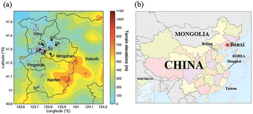
The city of Benxi, which is in Liaoning Province, is located on the edge of northeastern China (123°34ʹ-125°46ʹE, 40°49ʹ-41°35ʹN). Its total area is 8411.3 km², and the urban area is just 1526 km² (its dimensions are 27.1 km from west to east and 56.32 km from north to south). Benxi contains several types of terrain. Mountainous areas account for almost 80% of the area, the cultivated land area accounts for only 8.7%, and water and other land cover types account for 11.3%. These values indicate that the city of Benxi is a place with complex mountainous topography. Actually, the forest coverage in Benxi has reached more than 70%, and these forests are mainly distributed within the suburban area. That is the reason why the urban area is the target area for this study, rather than the whole city of Benxi. The urban area of Benxi mainly consists of four administrative districts (Xihu, Pingshan, Mingshan, and Nanfen), which are shown in Figure 1a. The terrain heights in the entire urban district show strong variations. The elevations are relatively low in the west and north, and they are higher in the east and southeast. The maximum elevation is 1002.78 m, the minimum elevation is 85 m, and the average elevation is 350 m. The blue dots (S1 and S2) located in the southern and central areas represent the geographical positions of meteorological observation stations where the meteorological data from 2012 used in this study were obtained. The black dots (S3, S4, S5, S6, S7, and S8) represent air quality monitoring sites, which are mostly distributed in the districts of Xihu, Pingshan, and Mingshan. They primarily provide air quality parameters related to high-priority pollutants (PM₁₀, SO₂, and NO_x) for this study.

Figure 1. (a) The urban area of Benxi (Xihu, Pinshan, Minshan, and Nanfen) and the locations of meteorological stations (blue dots), point sources (red dots), and air quality monitoring stations (black dots). (b) The location of the city of Benxi in China.

Benxi is located in the middle temperate zone and experiences an annual average temperature of 6.1–7.8 °C. The maximum temperature usually reaches 24.3 °C during the hottest month, July, and the minimum is −14.3 °C during the coldest month, January. In addition, the precipitation and rainfall in Benxi are sufficient, and the annual rainfall is 800–1000 mm. More than half of this amount occurs during July and August in the summer. Furthermore, the yearly dominant wind directions in the urban area of Benxi are mainly southwest, west, and northwest.

Methodology and data sources

Technical framework

Figure 2 shows the technical framework adopted in our study. The technical framework for urban air quality management, which is based on the integrated modeling tool mentioned above (WRF/CALPUFF), is described below and was used to provide control measures for improvement in air quality in our research. This technical framework consists of several components: a source emission inventory, an air quality modeling system, an evaluation approach for the analysis of source contributions, and the corresponding control measures.

Figure 2. Technical framework for air quality management based on the source apportionment of the pollutants PM₁₀, SO₂, and NO_x.

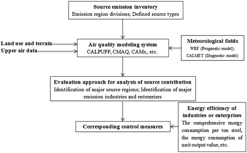
As seen in Figure 2, the emission inventory is the first important component in this framework. Briefly, an emission inventory represents an estimate of pollutant emissions that affect air quality on specific temporal and spatial scales. The emission inventory of the urban area of Benxi was set up on the basis of existing emission data obtained from the National Pollution Source Census (CCFNPSCD, 2011), the China Environmental Statistics, and the data contained in pollution discharge declarations and registrations, which represent the main data sources for building emission inventories in China. The National Pollution Source Census, which is performed by the Ministry of Environmental Protection and the National Bureau of Statistics, together with the China Environmental Statistics, covers the industrial sources, agricultural sources, and domestic sources and indicates the corresponding emissions and other basic data. The data from pollution discharge declarations and the registration of various enterprises, which is administered by local Environmental Protection Bureaus, systematically comprise the emission data related to various sources at the county level. Moreover, the technical method for building an emission inventory could be obtained from the technical guidance for emission inventories (MEPC, 2014) and other relevant published references (Lim and Boileau, 1999; Ohara et al., 2007; Tian et al., 2012; Zhang et al., 2014). We built the source database using GIS software. In this framework, the emissions from various sources were distributed over a grid with a resolution of 1 km × 1 km that covered our target area. The sources were spatially divided further according to administrative district, and the source types and corresponding emissions were also estimated, with the goal of determining the source apportionment for each pollutant. Additionally, in the absence of representative local emission factors, ranges of internationally reported values were considered and adjusted to account for case-specific conditions (El-Fadel and Abi-Esber, 2012; Whyatt et al., 2007).

The meteorological fields were mainly derived from numerical models, including the prognostic model WRF and the diagnostic model CALMET, both of which can be used for air quality modeling. The main air quality models currently include CALPUFF, CMAQ, CAMx (Comprehensive Air Quality Model with Extensions), etc., which have been applied in many other studies. In our study, the air quality modeling system consisted of WRF and CALPUFF. WRF was used to generate dynamic meteorological fields for CALMET that completely covered the study area. Data on topography (terrain height and land use–land cover types) and observed meteorological data (ground-based meteorological observational data and upper air data) were then collected and used as input data for the CALMET model to generate more precise hourly meteorological fields. The source emission inventory and the meteorological fields from the CALMET model were input into the CALPUFF module, which simulates the migration, diffusion, and transformation of pollutants in order to obtain hourly concentration values. Detailed information on the model setup is given below in the section “Model introduction and configuration.”

The evaluation approach for the analysis of source contributions made up the core of this technical framework. It helped to identify the source regions and industries that had adverse impacts on air quality, according to the spatial-temporal variations of pollutant concentrations and the contributions from each source category.

In the end, the entire air quality assessment was performed to finish the work of performing a quantitative source apportionment of atmospheric pollutants, as well as proposing corresponding control measures for consideration by local policy makers. Those source regions or industries that have great influence on air quality should be strictly controlled by local policy makers. Meanwhile, the energy and environmental efficiency of industries or enterprises, as assessed using metrics such as total energy consumption per ton of steel and energy consumption per unit of output value, should also be considered in the detailed control measures proposed. It is hoped that these control measures will help policy makers to improve urban air quality.

Model introduction and configuration

Weather Research and Forecasting (WRF) model

The WRF model is a next-generation meso-scale numerical weather prediction system designed for both atmospheric research and operational forecasting needs (Cipagauta et al., 2014), and the model serves a wide range of meteorological applications across scales from kilometers to thousands of kilometers (Giannaros et al., 2013; Kusaka et al., 2009; Winiarek et al., 2014). Its vertical coordinate is a terrain-following hydrostatic pressure coordinate, and the grid staggering is based on the Arakawa C-grid. The model uses the Runge-Kutta second- and third-order time integration schemes and second- to sixth-order advection schemes in both the horizontal and vertical directions.

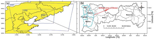
In this study, three one-way nested domains with 191 × 132, 295 × 208, and 61 × 118 grid points and grid spacings of 9, 3 and 1 km, respectively, were used, as shown in Figure 3a. The meteorological fields were provided by the WRF model, and the initial and lateral boundary conditions were obtained from the Global Forecast System Final Analyses of the National Centers for Environmental Prediction (NCEP), which have a horizontal resolution of 0.5° × 0.5°, at 6-hr intervals. The innermost domain, which provided adequate coverage over the urban districts of Benxi (the study area) and the surrounding rural areas, was centered at 124.76°E and 41.25°N, as shown in Figure 3b.

Figure 3. The simulation domains. (a) The three nested domains in WRF and (b) the urban area in the innermost domain (D03). The gray line in Figure 3(b) shows the main road.

Most of the physics schemes were used in the WRF model, such as the WRF single-moment six-class graupel microphysics scheme (Hong et al., 2004; Hong and Lim, 2006), the Dudhia short-wave radiation scheme (Dudhia, 1989), the Monin-Obukhov surface layer scheme (Monin and Obukhov, 1954), and the Yonsei University boundary layer scheme, which was used to represent the planetary boundary layer (PBL) over the domain (Noh et al., 2003). The Rapid Radiative Transfer Model long-wave radiation scheme (Mlawer et al., 1997) was applied in this model, and the Noah land surface model was also used to calculate the heat and moisture content of each subsoil layer (Kuang et al., 2013).

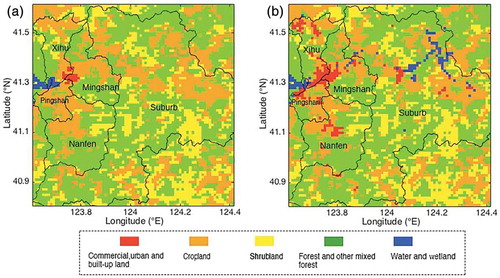
Previous work has also shown that there is an intimate correlation between land cover types and meteorological fields, especially wind speed and temperature, in the WRF model (Kuang et al., 2013). The default land use data from the United States Geological Survey (USGS) used in the WRF model are based on 1-km Advanced Very High Resolution Radiometer data obtained from 1992 to 1993, which are considered to be outdated, due to their failure to represent the rapid urban expansion in the past several decades in the urban area of Benxi. Realistic land use data based on the current status of land use in the city of Benxi (2010) were used to derive up-to-date urban land use categories and to replace the outdated land use categories provided by the USGS. The original land use data and the updated urban land use data are shown in Figure 4.

Figure 4. (a) Urban land use in the innermost domain using land use data from the USGS. (b) The updated land use data.

CALPUFF

The CALPUFF model is an advanced non-steady-state meteorological and air quality modeling system (Abdul-Wahab et al. 2010; Macintosh et al., 2010; Zhou et al., 2003). It has been adopted by the U.S. Environmental Protection Agency (EPA) and the Ministry of Environmental Protection of the People’s Republic of China (MEPC) as the preferred model for assessing the long-range transport of pollutants and their impacts on Federal Class I areas and on a case-by-case basis for certain near-field applications involving complex meteorological conditions (EPA, 2008). Compared with other models, CALPUFF is widely applicable, open-source, and has powerful simulation capabilities under non-steady-state conditions and in situations with complex terrain (Scire et al., 2000; Wang et al., 2006).

The CALPUFF model system is mainly composed of CALMET (a diagnostic three-dimensional meteorological module), CALPUFF (an air quality dispersion module), and CALPOST (a postprocessing package), as well as other useful processors. CALMET is a diagnostic wind field model with micrometeorological modules for overwater and overland boundary layers (Cui et al., 2011; Earth Tech, 2001; Scire et al., 2000). The CALMET model can use simulated fields from WRF, as well as observed data, as inputs to automatically generate hourly wind fields, mixing heights, and other three-dimensional micrometeorological parameters. The CALPUFF model is the core module of the whole air quality dispersion system, and it is a multilayer, multispecies non-steady-state Gaussian puff dispersion model that simulates the effects of temporally and spatially varying meteorological conditions on pollutant transport, transformation, and removal. Unlike traditional Gaussian plume models, CALPUFF simulates the continuous plume from a source as a series of discrete “puffs” (packets of pollutants) (Scire et al., 2000) that are transported and dispersed through a three-dimensional wind and micrometeorological field generated by the CALMET model. CALPOST postprocesses the results from the CALPUFF model, and it finally generates hourly, 24-hr, monthly, or yearly average concentrations of pollutants within specified horizontally gridded cells.

The terrain and land use input data were derived from USGS data. In particular, the land use data were corrected using realistic land use types for this case study, which treats the urban area of Benxi, in order to improve the performance of this simulation (Figure 4). The observed meteorological data from stations S1 and S2 were not input into the CALMET module, and they were mainly used to verify the performance of CALMET simulation. The simulated domain was slightly smaller than that used in WRF, and it was gridded and specified at the southwestern corner (4498.76 km south and 549.73 km west in Universal Transverse Mercator [UTM] zone 51), and it contained 56 grid cells from east to west and 65 grid cells from south to north, with a resolution of 1 km. In the vertical dimension, the nine height layers incorporated into the CALMET model had their boundaries at elevations of 10, 20, 50, 100, 200, 500, 1000, 1500, and 2000 m.

In this study, the dispersion options, including wet and dry deposition, were selected independently. For wet deposition, both scavenging coefficients for liquid precipitation were set to 1 × 10⁻⁴, 3 × 10⁻⁵, and 3 × 10⁻⁵ for PM₁₀, SO₂, and NO_x, respectively (Hao et al., 2007; Zhou et al., 2003). The dry deposition parameters included the reference cuticle resistance and reference ground resistance (Lee et al., 2014), and the dry deposition velocities for each pollutant (PM₁₀, SO₂, and NO_x) were calculated separately using the resistance model internal to CALPUFF. Chemical transformations, such as the conversion of SO₂ to sulfate and the conversion of nitrogen oxides to nitrate aerosols, were computed internally. However, the chemical reaction options (such as the background concentrations of precursor gases, including ammonia [NH₃], hydrogen peroxide [H₂O₂], nitric oxide [NO], and nitrogen dioxide [NO₂] and secondary organic aerosols) were not considered in this study, and all of the emission sources were considered to be point and area sources (Lee et al., 2014). The other chemical transformation options were set to their default values and computed internally in the CALPUFF model.

Analysis of the emission inventory

The sources in our study were categorized into four different districts (Xihu, Pingshan, Mingshan, and Nanfen), including both point and area sources. This categorization was described in terms of districts. According to another classification method, in which the sources were described in terms of types, the sources were grouped into categories, which included the Bengang Group, large point sources, small point sources, and area sources. The district-based method provided a basis for identifying the major source regions based on emission contributions and their contributions to pollutant concentrations, and the type-based method mainly provided an easy method for understanding the effects of various industrial sources on local urban air quality. Figure 5 shows the emissions and emission contributions from each source category using the two different classification methods (the district-based method and the type-based method) for the various sources. Using the district-based method, the total emissions of PM₁₀, SO₂, and NO_x were estimated to be 104410.6, 40169.7, and 38872.7 metric tons/year. Large emission contributions were noted in Pingshan and Xihu, due to the presence of the Bengang Group, power plants, and other industrial sources, which used excessive amounts of fossil fuels, including coal, gas, and oil, to produce energy. Using the type-based method, the emission contributions from point sources for each pollutant exceeded 89%, of which the Bengang Group accounted for more than 42%. Apparently, the air pollution was mainly caused by point sources, rather than area sources, in terms of emissions. In addition, the total emissions of PM₁₀ were far higher than those of SO₂ and NO_x, which indicated that PM₁₀ was clearly the primary pollutant responsible for air pollution in the urban area of Benxi.

Figure 5. (a) The sources categorized using the district-based method (Xihu, Pingshan, Mingshan, and Nanfen) are shown as emissions (metric tons/year) and emission contributions from each source category. (b) The sources categorized using the type-based method (the Bengang Group, the large point sources, the small point sources, and the area sources) are shown as emissions (metric tons/year) and emission contributions from each source category.

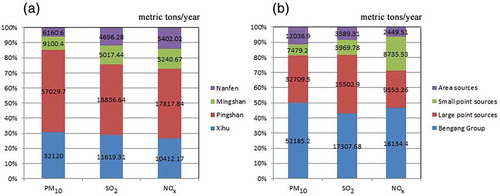
In particular, the Bengang Group included 24 large point sources that represented its various subsidiaries, and these point sources were specifically excluded from the large point sources group in this study. The large point sources included 36 various point sources, most of which represented the smelting and processing of ferrous metals, the production and distribution of electrical and heat energy, the mining and washing of coal, etc. The small point sources were small-sized industries that produced relatively small amounts of emissions compared with those of the large point sources, and the area sources included residential sources, traffic sources, and other unorganized sources. To further understand the characteristics of the industry operating in the urban area of Benxi, we analyzed the energy consumption status of various industries in 2012 (Table 1). Apparently, the iron-making industries, most of which belonged to the Bengang Group, accounted for most of the energy consumption, i.e., 62.91% of the total. On the other hand, the other industries, such as the smelting and processing of steel, power plants, etc., only accounted for the remainder of the energy consumption (37.08%), although they had an advantage in terms of their number. Without question, the Bengang Group and the numerous industries listed in Table 1 were the industries that displayed large amounts of energy consumption and emissions.

Table 1. Energy consumption status of industries in the urban area of Benxi in 2012.

Industry	Number	Energy consumption (tce)	Proportion of energy consumption (%)	Cumulative sum (%)
Iron-making	13	8,395,688	62.91	62.91
Smelting and processing of steel	9	1,167,974	8.75	71.66
Power plants	4	958,048.4	7.18	78.84
Production and distribution of heat energy	40	594,796.5	4.46	83.3
Coking	2	577,244.8	4.33	87.63
Manufacturing of cement	5	333,173.2	2.50	90.13
Mining and dressing of iron ores	40	281,247.2	2.11	92.24
Steel-making	5	214,785.5	1.61	93.85
Manufacturing of lime and gypsum	7	208,349	1.56	95.41
Other	151	613,692.4	4.59	100
Total	276	13,344,999	100

The temporal variability of point sources and vehicle sources was considered in our emission inventory. For the Bengang Group, the daily variation coefficient was determined by the monitoring emission data. In addition, the daily variation coefficient of pollution emissions from large point sources was mainly determined by the daily variations in the electrical load, whereas the daily variation coefficient of the small point sources was determined by the diurnal variation of the industrial production process in general. These values were then smoothed before they were entered into the model. For the vehicle sources, the daily variation coefficient was determined based on the diurnal variation of traffic flow. The emission inventory was constructed in the designated format. Point sources were associated with the parameters of stack height, stack diameter, emission rate, gas exit velocity and temperature, which were needed to simulate the transport, dispersion, chemical reaction, and deposition of air pollutants under the temporally and spatially varying meteorological conditions. In addition, the area sources included vehicle sources, residential sources, and miscellaneous sources, which were also considered to be area sources because of their scale and the difficulty of specifically locating each source. These area sources were calculated and allocated within a 1 km × 1 km grid using GIS software. The total emissions from various sources were estimated essentially by multiplying the emission factors and the relevant activity data, considering the removal efficiencies of control devices (Lee et al., 2011).

Evaluation approach for the analysis of source contributions

The brute-force method, which has been widely applied in source apportionment to compare the different impacts of various sources on pollutant concentrations (Kwok et al., 2014; Zhang et al., 2014), was applied in the CALPUFF module. Each source category was simulated individually in CALPUFF without considering the impact of other source categories for each pollutant. Thus, for each simulation, when one source category was run, the other source categories were not considered.

Using the district-based method, the contributions to pollutant concentrations (PM₁₀, SO₂, and NO_x) at receptor n (S3, S4, S5, S6, S7, and S8) from source area i (Pingshan, Mingshan, Xihu, and Nanfen) were characterized as S_a(i, n). Using the type-based method, the contributions to pollutant concentrations at receptor n from source j (the Bengang Group, large point sources, small point sources, and area sources) were characterized as S_b(j, n). The contribution rate of each source category at receptor n can be calculated as

(1)

(2)

Here, C_a(i, n) represents the contributions of PM₁₀, SO₂, and NO_x to receptor n using the district-based method, whereas C_b(j, n) represents the contributions of PM₁₀, SO₂, and NO_x to receptor n using the type-based method.

Results and analysis

Verification of meteorological fields and concentration simulations

To verify the reliability of the case-specific simulations, we used statistical indexes to evaluate the performance of the combined model by comparing the simulated results, including both the meteorological fields (CALMET) and the concentration fields (CALPUFF), with the observed values. The indexes included the index of agreement (IOA), the Pearson correlation coefficient (CC), the mean bias (MB), and the root mean square error (RMSE). The formulas describing the above indexes are given below (Cai and Xie, 2010; Gupta and Mohan, 2013).

(3)

(4)

(5)

(6)

S_i and O_i represent the simulated and observed values; and are the mean values of the simulated and observed values; and i and n are the indexes of the elements and the number of samples, respectively.

The value of the IOA always ranges from 0.0 to 1.0 (a value of 1.0 represents perfect agreement between the predicted and observed values, whereas a value of 0.0 is the theoretical minimum for an inaccurate prediction), and it reflects the degree to which the simulated values are accurate, as assessed using the observations. Moreover, the simulated results are credible to some degree when the IOA is above 0.5 (Levy et al., 2009; Willmott, 1984; Zawar-Reza et al., 2005). The CC indicates the correlation and degree of consistency between the simulated values and the observed values, and it ranges from −1.0 to 1.0 (a value of 1.0 indicates a positive correlation between the predicted and observed values, whereas a value of −1 indicates a negative correlation). Therefore, a particular simulation was counted as a success if both the IOA and the CC were close to 1. Furthermore, the MB represents the systematic error, whereas the RMSE reflects the square root of the average squared error. The closer the values of these indexes are to 0, the better the match of the simulated values to the data is.

The verification of meteorological fields

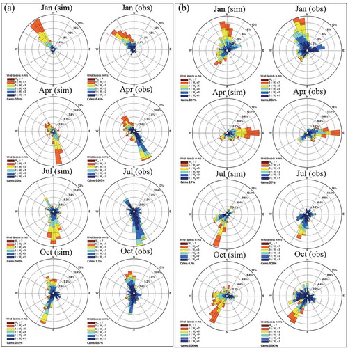
Figure 6 shows wind roses constructed from hourly simulated and observed data during various periods (January, April, July, and October; Jan, Apr, Jul, and Oct hereafter) in the CALMET model at the locations of S1 (Figure 6a) and S2 (Figure 6b) (see Figure 1). It can be seen that the wind speeds and directions generally agreed well with the observations. To further evaluate the credibility of the meteorological simulations, the four statistical indexes (IOA, CC, RMSE, and MB) were used to compare the hourly simulated values (wind speed and temperature) with the observed values at sites S1 and S2 during four different periods (Jan, Apr, Jul, and Oct), as shown in Table 2. For the sites S1 and S2, the averaged IOA values were 0.82 and 0.89 (0.76–0.89 and 0.85–0.91) for wind speed and 0.96 and 0.95 (0.95–0.98 and 0.94–0.96) for temperature. The averaged values of the RMSE, the MB, and the CC were 1.22 m/sec, 2.04 m/sec, and 0.82 for wind speed and 2.95 °C, −0.59 °C, and 0.95 for temperature at site S1. The corresponding values at site S2 were 1.27 m/sec, 1.92 m/sec, and 0.82 for wind speed and 1.89 °C, 0.45 °C, and 0.98 for temperature. The IOA values for wind speed and temperature were relatively high, indicating a high degree of consistency and correlation between the simulated and observed values. Meanwhile, the simulated wind speeds were probably overestimated because of the positive average MB values for wind speed (2.04 m/sec at S1 and 1.92 m/sec at S2). The low RMSE values obtained during various periods for wind speed and temperature also showed the reliability of the meteorological simulations produced by CALMET. Based on these results, the simulated data showed considerable agreement with the observed data, which provided a strong foundation for predicting the dispersion and concentration distributions of PM₁₀, SO₂, and NO_x in CALPUFF.

Table 2. Statistical verification of CALMET simulations at meteorological monitoring sites S1 and S2.

		S1				S2
Period	Parameter	RMSE	MB	CC	IOA	RMSE	MB	CC	IOA
Jan	Wind speed	1.23	2.13	0.87	0.76	1.56	2.65	0.73	0.91
	Temperature	1.58	−0.08	0.93	0.96	1.83	−1.23	0.97	0.95
Apr	Wind speed	1.45	1.45	0.79	0.87	0.87	1.65	0.87	0.89
	Temperature	2.43	−1.19	0.98	0.95	1.56	1.13	0.98	0.96
Jul	Wind speed	0.98	2.12	0.86	0.76	1.23	2.18	0.9	0.89
	Temperature	2.14	−1.15	0.96	0.95	2.81	0.94	0.97	0.94
Oct	Wind speed	1.23	2.45	0.76	0.89	1.41	1.21	0.78	0.85
	Temperature	3.24	0.07	0.94	0.98	1.37	0.94	0.98	0.94
Average	Wind speed	1.22	2.04	0.82	0.82	1.27	1.92	0.82	0.89
	Temperature	2.35	−0.59	0.95	0.96	1.89	0.45	0.98	0.95

Note. MB: °C for temperature, m/sec for wind speed; RMSE: °C for temperature, m/sec for wind speed.

Figure 6. Wind roses constructed from simulated (left) and observed (right) data from meteorological simulations in CALMET at sites S1 (a) and S2 (b). S1 represents the meteorological fields far away from the central urban area, whereas S2 represents the meteorological fields in the adjacent areas of Xihu, Pingshan, and Mingshan.

The verification of the concentration fields

During the simulation period, we selected the days during which the air pollution was relatively serious by looking to see whether the AQI value exceeded 50. Figure 7 demonstrates the close relationship between the observed values and the simulated values at six ambient monitoring stations during selected periods. It is easy to see that the simulated values are generally lower than the observed values during various periods. One major reason might be due to the overestimated wind speed (Gao et al., 2015; Tasić et al., 2013), as shown in Figure 6. Another major reason can also account for this phenomenon: the emission sources in the surrounding area, together with biogenic and natural emissions, were not considered because of the difficulty of making quantitative predictions of concentrations in the strict sense caused by uncertain and variable emissions, such as the temporary construction activity in vicinity of the receptors (Kesarkar et al., 2007).

Figure 7. Comparison of daily average values with observed values for PM10, SO2, and NOx at six stations (S3, S4, S5, S6, S7, and S8) during the four selected periods, specifically Jan (13–16), Apr (12–18), Jul (14–20), and Oct (12–18).

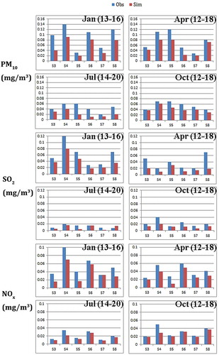
The statistical analyses for each pollutant were calculated between the CALPUFF simulations and observations, based on hourly average concentrations at selected times during typical months at three key stations (S3, S4, and S6, which are shown in Figure 1, represent the air quality in Xihu, Pingshan, and Mingshan, respectively; the air pollution in these districts was relatively serious and a source of public concern). Table 3 summarizes the values of the IOA, the CC, the RMSE, and the MB for each pollutant during various selected periods. The values of the IOA and the CC were generally high at the three stations for each pollutant, with the exception of S6 (where the average IOA value was 0.564 for PM₁₀, and the average CC values were 0.4, 0.598, and 0.545 for PM₁₀, SO₂, and NO_x). In particular, the simulated values from S3 showed better agreement with the observed data than those at the other two stations (S4 and S6), with average IOA values (0.732, 0.843, and 0.691 for PM₁₀, SO₂, and NO_x) and CC values (0.673, 0.68, and 0.567 for PM₁₀, SO₂, and NO_x). The IOA values were nearly 0.5, meaning that the simulated results were generally credible compared with the observed values, although the simulated data were not perfect. The average RMSE values ranged from 0.008 to 0.023 mg/m³ for PM₁₀, 0.023 to 0.095 mg/m³ for SO₂, and 0.012 to 0.034 mg/m³ for NO_x during the various periods. Furthermore, the average MB values for PM₁₀ (−0.016, −0.032, and −0.021 mg/m³ for S3, S4, and S6), SO₂ (−0.004, −0.013, and −0.023 mg/m³ for S3, S4, and S6), and NO_x (−0.012, −0.013, and −0.023 mg/m³ for S3, S4, and S6) reflected underestimates of the actual air pollution at the three key stations. In addition, the IOA values during the four periods ranged from 0.435 to 0.678 for PM₁₀, 0.563 to 0.786 for SO₂, and 0.398 to 0.864 for NO_x, and the CC values ranged from 0.567 to 0.786 for PM₁₀, 0.467 to 0.675 for SO₂, and 0.337 to 0.679 for NO_x. In general, the results show that the concentration field for each pollutant simulated in this study shows good agreement with the actual air pollution situation.

Table 3. Statistical verification of CALPUFF simulations at the air quality monitoring stations (S3, S4, and S6).

	PM10				SO2				NOx
Station/Period	IOA	CC	RMSE	MB	IOA	CC	RMSE	MB	IOA	CC	RMSE	MB
Stations^a
S3	0.732	0.673	0.008	−0.016	0.843	0.680	0.095	−0.004	0.691	0.567	0.034	−0.012
S4	0.623	0.578	0.011	−0.032	0.745	0.734	0.023	−0.013	0.634	0.689	0.023	−0.013
S6	0.564	0.4	0.023	−0.021	0.652	0.598	0.045	−0.023	0.543	0.545	0.012	−0.023
Periods^b
Jan (13–16)	0.678	0.786	0.035	−0.032	0.645	0.563	0.038	−0.021	0.754	0.534	0.043	−0.037
Apr (12–18)	0.435	0.567	0.027	−0.023	0.563	0.467	0.021	−0.018	0.456	0.432	0.028	−0.023
Jul (14–20)	0.578	0.678	0.014	−0.012	0.786	0.675	0.011	−0.008	0.864	0.679	0.032	−0.012
Oct (12–18)	0.554	0.598	0.021	−0.014	0.782	0.598	0.009	−0.024	0.398	0.337	0.016	−0.023
Average	0.561	0.657	0.024	−0.020	0.694	0.576	0.020	−0.018	0.618	0.496	0.03	−0.024

Note. ^aStation values are based on hourly concentrations during the selected periods (Jan (13–16), Apr (12–18), Jul (14–20), and Oct (12–18)).

^bPeriod values are based on the average concentrations at the three stations (S3, S4, and S6); RMSE (mg/m³), MB (mg/m³).

Concentration distributions of air pollutants

Figure 8 shows the distributions of concentrations and the meteorological fields for each pollutant during the different periods. Considering the average of all of the time periods, PM₁₀ had higher average concentrations than SO₂ and NO_x, as well as a larger radius of impact, mainly owing to the greater total amount of emissions. High concentrations of each pollutant tended to appear in the urban centers, compared with those occurring in the surrounding area. In particular, the concentrations in the southeastern part of the urban area of Benxi, i.e., most of the district of Nanfen, were very low. The air pollutants, especially PM₁₀, mainly transformed from the source regions towards the northeast and southeast, and the corresponding concentrations gradually decreased with increasing distance from the center.

Owing to the variations in meteorological conditions between the different seasons, the seasonal pattern for each pollutant was different. During Jan (13–16), the pollutants were mainly affected by winds from the northwest and southwest, and the concentrations in the southeast and northeast were relatively low. The maximum 24-hr average concentrations for PM₁₀, SO₂, and NO_x were 0.21, 0.18, and 0.16 mg/m³. These elevated concentrations all occurred in the central area of the urban area of Benxi and exceeded the national 24-hr averaged values of 0.15, 0.15, and 0.1 mg/m³, respectively, by considerable margins. This result indicated that the air quality was substantially influenced by the wind direction, wind speed, and topography (Chuang et al., 2011; Gopalaswami et al., 2015; Tartakovsky et al., 2016). During Apr (12–18), the degree of air pollution was limited compared with the pollution that occurred during Jan (13–16), and the highest concentrations occurred west of the urban area of Benxi because the dominant wind direction was from the northeast. The high concentrations for each pollutant were distributed in Pingshan and parts of the areas of Xihu and Mingshan, and the 24-hr average concentrations for each pollutant in the eastern part of the urban area of Benxi were generally below 0.01 mg/m³. During Jul (14–20), the air pollutants were mainly influenced by the prevailing wind directions from the south and southwest, and the scopes of the air pollution were very limited. The high PM₁₀ concentrations were concentrated in the central urban area, and the SO₂ and NO_x mainly occurred to the central urban area and south. Noticeably, the 24-hr average concentrations of SO₂ and NO_x during Jul (14–20) in the east were also almost as low as 0.01 mg/m³. Previous studies have shown that summer is associated with the highest mixing height, which is conducive to pollutant diffusion (Lokeshwari et al., 2014; Protonotariou et al., 2005). During Oct (14–20), the radius of the air pollution was slightly smaller than that during Jan (13–16), and the air pollutants spread to the east and southeast. High concentrations of PM₁₀ tended to appear in Pingshan and Nanfen, whereas high concentrations of SO₂ and NO_x tended to emerge in Mingshan and part of the area of Nanfen.

Analysis of source contributions

To determine the differences in the degrees to which various sources in a particular area of concern have negative impacts on air quality and to identify the major types of sources that directly affect air quality, the pollution sources were classified using the district-based method and the type-based method (see Figure 5). Moreover, we simulated the source contributions of each source category at six air monitoring stations under the same emission and meteorological conditions. Figure 9 shows the contributions of each source category to the six monitoring sites using the district-based method and the type-based method on average for all four simulation periods.

Figure 8. Spatial distributions of the simulated concentration fields for PM₁₀, SO₂, and NO_x and meteorological fields during Jan (13–16), Apr (12–18), Jul (14–20), and Oct (12–18).

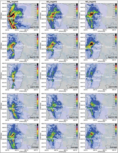
Figure 9. Contributions of PM₁₀, SO₂, and NO_x to all monitoring stations from different source categories using the district-based method and the type-based method (PM₁₀ (a), SO₂ (a), and NO_x (a) belong to the district-based method, and PM₁₀ (b), SO₂ (b), and NO_x (b) belong to the type-based method), averaged over the four periods.

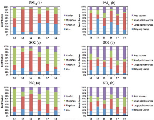
Using the district-based method, Figure 9 shows the contributions, averaged over the four periods, from the four districts (Xihu, Pingshan, Mingshan, and Nanfen) to the six sites (S3, S4, S5, S6, S7, and S8). Obviously, the PM₁₀ concentrations at S3 and S8 mainly came from Xihu, Pingshan, and Mingshan, whereas the SO₂ and NO_x concentrations mostly came from Mingshan. Additionally, the concentrations of PM₁₀, SO₂, and NO_x at S4 and S5 largely came from Pingshan, the PM₁₀ concentrations at S6 and S7 came from Pingshan and Xihu, and the SO₂ and NO_x concentrations were mainly derived from Pingshan and Mingshan. Furthermore, the average contributions of the four districts (Xihu, Pingshan, Mingshan, and Nanfen) to all of the sites were 18.38%, 66.44%, 12.08%, and 3.11% for PM₁₀; 14.73%, 47.45%, 26.73%, and 11.1% for SO₂; and 15.56%, 40.2%, 29.48%, and 14.75% for NO_x. Obviously, these results show that Pingshan had a considerable influence on the air quality represented by the monitoring sites. This influence reflected the excessive emissions from the Bengang Group, as well as an unreasonable layout of industries and adverse topographic conditions that resulted in the high contribution levels. In addition, for SO₂ and NO_x, the concentrations from Mingshan were relatively high in contrast to that of PM₁₀, owing to the sites (S3, S7, and S8) that were located in Mingshan and the presence of several iron-producing facilities and large power plants.

Using the type-based method, the contributions from various source categories to the pollutant concentrations at the sites were significantly different. For PM₁₀, the contributions from the Bengang Group and the large point sources at all sites were apparently higher, whereas the contributions from the small point sources and the area sources were very limited. For instance, the concentration contributions from the Bengang Group reached 56.72% and 41.57% at sites S4 and S6, whereas the contributions from the large point sources reached 61.1% and 60.84% at sites S3 and S8, respectively. For SO₂ and NO_x, the concentration contributions from the area sources at all sites increased remarkably compared with those of PM₁₀ and were as high as the total contributions from the large point sources and the small point sources. For example, the contributions from the area sources at S5, S7, and S8 were 49.02%, 49.76%, and 44.53% for SO₂ and 45.03%, 39.12%, and 35.23% for NO_x, respectively. Consequently, the area sources, which mainly consisted of vehicle sources and domestic sources that accounted for smaller amounts of emissions (see Figure 5), still had considerable impacts on air quality, owing to the low emission heights and the lack of effective control measures. The average contributions from the Bengang Group, the large point sources, the small point sources, and the area sources to all sites were 41.52%, 32.79%, 9.71%, and 15.98% for PM₁₀; 21.56%, 28.22%, 12.08%, and 38.15% for SO₂; and 21.24%, 28.5%, 21.74%, and 28.53% for NO_x.

Moreover, we also considered the differences in source contributions during various periods that represented various typical seasons. Table 4 shows the average contributions of PM₁₀, SO₂, and NO_x during each period using the district-based method and the type-based method. In the case of the district-based method, the average PM₁₀ contribution from Pingshan to all sites reached its peak (82.65%) during Jul (14–20); on the other hand, the minimum (40%) was achieved during Apr (12–18). Meanwhile, the average contributions from Xihu and Mingshan synchronously reached their maxima of 28.53% and 26.93% during Apr (12–18). The average contribution from Nanfen was always low, and its maximum contribution was only 4.55%, which occurred during Apr (12–18). For SO₂, the maximum contributions from the four districts (Xihu, Pingshan, Mingshan, and Nanfen) appeared during Oct (12–18) (20.62%), Apr (12–18) (51.35%), Jul (14–20) (32.47%), and Oct (12–18) (20.62%), respectively. In addition, the maximum NO_x contributions from the four districts emerged during Oct (12–18) (29.24%), Jan (13–16) (46.47%), Jul (14–20) (35.02%), and Oct (12–18) (28.24%), respectively. Notably, although the contributions from each district varied with time, the contribution of Pingshan to each pollutant was the largest during each of the four different periods. Using the type-based method, the average contributions of PM₁₀ from the Bengang Group, the large point sources, the small point sources, and the area sources during the various periods ranged from 26.73% to 63.19%, 21.87% to 44.03%, 2.14% to 28.48%, and 9.14% to 26.82%; the SO₂ average contributions ranged from 19.57% to 24%, 24.52% to 32.74%, 6.02% to 18.57%, and 33.87% to 43.59%; and the NO_x average contributions ranged from 19.18% to 23.89%, 18.70% to 37.56%, 8.18% to 31.37%, and 21.85% to 31.1%. Overall, the Bengang Group and the large point sources were always major sources of PM₁₀ pollution, whereas all the source types, especially the large point sources and the area sources, had considerable impacts on the SO₂ and NO_x concentrations during various periods.

Table 4. Averaged contributions of PM₁₀, SO₂, and NO_x during each period using the district-based method and the type-based method.

		District-based method (%)				Type-based method (%)
Pollutant	Period	Xihu	Pingshan	Mingshan	Nanfen	Bengang Group	Large point sources	Small point sources	Area sources
PM10	Jan (13–16)	14.13	76.69	6.89	2.29	32.79	24.56	28.48	14.17
	Apr (12–18)	28.53	40	26.93	4.55	63.19	21.87	5.80	9.14
	Jul (14–20)	5.11	82.65	9.08	3.17	26.73	44.03	2.42	26.82
	Oct (12–18)	25.74	66.43	5.41	2.42	43.36	40.70	2.14	13.80
	Average	18.38	66.44	12.08	3.11	41.52	32.79	9.71	15.98
SO2	Jan (13–16)	18.56	49.88	26.75	4.80	24	29.83	6.02	40.15
	Apr (12–18)	3.86	51.35	29.97	14.83	21.98	32.74	11.41	33.87
	Jul (14–20)	15.86	47.53	32.47	4.13	19.57	24.52	12.31	43.59
	Oct (12–18)	20.62	41.03	17.73	20.62	20.67	25.78	18.57	34.99
	Average	14.73	47.45	26.73	11.1	21.56	28.22	12.08	38.15
NOx	Jan (13–16)	13.29	46.47	33.57	6.67	23.89	37.56	8.18	30.37
	Apr (12–18)	4.40	42.92	34.01	19.67	19.18	30.88	18.84	31.1
	Jul (14–20)	15.32	45.22	35.02	4.43	21.96	18.70	28.56	30.79
	Oct (12–18)	29.24	26.20	15.31	28.24	19.92	26.86	31.37	21.85
	Average	15.56	40.2	29.48	14.75	21.24	28.5	21.74	28.53

Note. The values in this table are based on the average contributions from all monitoring sites during each period.

Corresponding control measures

Identification of key areas for air pollution control

It is of great significance to identify the key areas for air pollution control in air quality management. In the management structure used in environmental protection in China, which has three levels (provinces, prefecture-level cities, and districts or counties), districts and counties, which are responsible for local ecological and environmental protection, become the basic platforms or units for the specific implementation of environmental protection measures. Consequently, to identify the key areas for air pollution control on the district or county scale in China would be very instructional and effective.

Using the technical framework adopted in our study, it was not difficult to identify the key areas for air pollution control. Table 5 shows the emission contributions and source contributions from each district. The pollutant emissions mainly came from Pingshan and Xihu, which contributed more than 70% of each pollutant when taken together (85.38% for PM₁₀, 75.82% for SO₂, and 72.63% for NO_x). The source contributions indicated that Xihu and Pingshan had considerable impacts on the PM₁₀ concentrations (18.38% and 66.44%), whereas Mingshan and Pingshan (26.73% and 47.45% for SO₂ and 29.48% and 40.2% for NO_x) had considerable impacts on the concentrations of SO₂ and NO_x. Hence, given the emission contributions and source contributions from each district, Pingshan could be identified as a key area for air pollution control, where strict cuts in the emissions of pollutants (PM₁₀, SO₂, and NO_x) might be considered. In addition, the emissions for each pollutant from Xihu were slightly lower than those from Pingshan, as was the PM₁₀ concentration contribution from Xihu (18.38%). Consequently, emission controls on particulate matter in Xihu should be another important aspect of the air quality management system of the urban area of Benxi. Furthermore, although the SO₂ and NO_x emissions in Mingshan were limited, the concentration contributions from Mingshan were relatively high, and they were only slightly lower than those of Pingshan. Without a doubt, the total emissions of SO₂ and NO_x from Mingshan should be controlled.

Table 5. The emission contributions and source contributions from each district of the urban area of Benxi.

	Emission contributions (%)				Source contributions (%)
Pollutant	Xihu	Pingshan	Mingshan	Nanfen	Xihu	Pingshan	Mingshan	Nanfen
PM10	30.76	54.62	8.72	5.9	18.38	66.44	12.08	3.11
SO2	28.93	46.89	12.49	11.69	14.73	47.45	26.73	11.1
NOx	26.79	45.84	13.48	13.9	15.56	40.2	29.48	14.75

Note. The source contributions are based on the average contributions of each district to all of the monitoring stations during the various simulation periods (for definitions of the periods, refer to Table 4).

The key industries and enterprises for air pollution control

Table 6 shows the emission contributions and source contributions from each source category (the type-based method). As one of the largest iron and steel enterprises in China, the Bengang Group was the largest point source in the urban area of Benxi, and it contributed 50%, 47%, and 43% of the emissions of PM₁₀, SO₂, and NO_x, respectively. The source apportionment showed that the Bengang Group had a considerable impact on urban air quality, which could be explained in terms of the source contribution of each pollutant (41.52% for PM₁₀, 21.56% for SO₂, and 21.24% for NO_x). In this study, energy and environmental efficiency is also an important indicator to identify the key industries or enterprises. The comprehensive energy consumption per ton of steel reached 0.72 tce/t (ton of standard coal equivalent per ton of output) in 2012. This value is still considerably higher when compared with the advanced energy consumption level, which is less than 0.6 tce/t (Shanghai Municipal Commission of Economy and Informatization [SHEITC], 2011) in China, and the total energy consumption of the steel industry accounted for 79.71% of the total energy consumed by industrial activities in the urban area of Benxi. In addition, for the Bengang Group, the energy consumption per unit output value was 1.72 tce/10⁴￥, which was also much higher than the domestic advanced level of 0.96 tce/10⁴￥ (SHEITC, 2011). Consequently, the Bengang Group is clearly a key control object. Optimizing the energy structure (increasing the proportion of clean energy and reducing the dependence on traditional energy sources, such as coal and other fossil fuels), increasing the use of advanced production technologies (eliminating outdated technology and equipment), and the promotion of dust removal and the purification efficiency of pollutants would be very effective in cutting down the emissions of pollutants from the Bengang Group.

Table 6. The emission contributions and source contributions from each source category.

	Emission contributions (%)				Source contributions (%)
Pollutant	Be	La	Sm	Ar	Be	La	Sm	Ar
PM10	49.98	31.33	7.16	11.53	41.52	32.79	9.71	15.98
SO2	46.65	24.58	22.47	6.30	21.56	28.22	12.08	38.15
NOx	43.09	38.59	9.88	8.44	21.24	28.5	21.74	28.53

Note. The source contributions are based on the averaged contribution from each source category to all of the monitoring stations during the various simulation periods (These periods refer to Jan (13–16), Apr (12–18), Jul (14–20), and Oct (12–18) in Table 4), and Be, La, Sm, and Ar represent the Bengang Group, the large point sources, the small point sources, and the area sources, respectively.

The emission contributions for each pollutant from the large point sources all accounted for more than 24%, and the concentration contributions exceeded 28%, averaged over all of the periods (see Table 6). In addition, industrial activities related to iron-making, energy production, the smelting and processing of steel, mining, and the production and distribution of heat energy accounted for most of the emissions from the large point sources, as well as the total energy consumption from all urban industries (see Table 1). Furthermore, these industries consumed very large amounts of energy per unit output value, and they displayed high concentration contributions to air quality among the large point sources. In light of their emission contributions and source contributions to air quality, the large point sources might also be subjected to emissions cuts, and the importance of this measure was only slightly smaller than that of the Bengang Group. This finding is especially true of industrial activities related to iron-making, energy production, the smelting and processing of steel, mining, and the production and distribution of heat energy, etc., that had high comprehensive energy consumptions and are thought to be key industries for saving energy and reducing emissions.

Although the emission contributions from the area sources (12% for PM₁₀, 6% for SO₂, and 8% for NO_x) were relatively low, their impacts on air quality were significant. The concentration contributions averaged over the four periods were 38.15% and 28.53% for SO₂ and NO_x, respectively, which were higher than those of the other source types (see Table 6). The area sources mainly included domestic sources, vehicle sources, and other unorganized sources, which were easy to consider as a group because of their low emission heights and because they are concentrated in the central part of the urban area of Benxi. Hence, the impact of the area sources on urban air quality should be carefully considered. Implementing vehicle emission standards, accelerating the elimination of old vehicles, improving residential energy efficiency, and promoting the use of central heating will greatly reduce pollutant emissions, especially the emissions of SO₂ and NO_x; thus, the urban air quality will be improved considerably. In addition, the area sources were mainly distributed within urban centers, so the districts of Xihu, Pingshan, and Mingshan were expected to cooperate to take up the responsibility for the air quality improvement.

As for the small point sources, their impact on air quality was relatively limited in terms of their emission contributions and source contributions, but their average NO_x contributions to the sites reached 21.74%, which should draw considerable attention.

Discussion

Remarkably, many approaches have always been useful for air quality management and improvement (Behera et al., 2010; Huang et al., 2012; Titov et al., 2007). The source apportionment of pollutants has been one of the most widely applied approaches used in studies of air quality management. Lee et al. (2014) evaluated the concentrations and source contributions from PM₁₀ and SO₂ emitted from industrial complexes to prioritize emission control and mitigation efforts for air quality improvement on small scales. Huang et al. (2012) studied the contributions from various sources in Beijing and systematically identified the local PM₁₀ emission sources that were of high priority for regulation in urban air quality management. All of these studies on emission source apportionment discussed the impacts of various sources on air quality and quantified the source contributions for different source categories. It can be seen that the quantitative simulation and analysis of air pollution, especially the quantitative analysis of pollutant source apportionment, are of great significance and have been widely applied in the world. Overall, this approach of using source apportionment based on models can provide better visually represented and quantitative data support for developing effective air quality management policies at different geographic scales. Based on this approach, this paper built a general technical framework for air quality management systems (see Figure 2). This framework is simple and easily understood, and it could be widely applied in studies of air quality management systems. It could be especially useful in many cities, such as Benxi in China. The technology and knowledge involved in this framework are quite mature, and they have been widely used in practice; hence, their use will reduce the costs to policy makers in China.

Based on this case study, some key factors should be considered for more effective implementation of this framework. First, this study showed that refinement of the emission inventory was important for improving the accuracy of the numerical simulation of air quality. Therefore, using a high spatial resolution could provide more accurate source contributions to pollutant concentrations (Pérezlanda et al., 2007; Tan et al., 2014). Hence, our modeling resolution was 1 km × 1 km, providing better performance in air quality simulations and an improved basis for calculating source contributions. In addition, it is crucial to establish a source classification system that meets the effective control requirements of the local atmospheric environment. The classification system should be based on the current situation, including air pollution, the characteristics of the industrial structure, the patterns and structure of energy consumption, and pollutant emissions.

Conclusion and limitations

In this study, the integrated model WRF/CALPUFF was utilized to develop a framework for improving the air quality management system in China. This framework consisted of a source emission inventory, an air quality modeling system, an evaluation approach for the analysis of source contributions, and the corresponding control measures at different levels, including districts, industries, and enterprises. In this case study, which treats the urban area of Benxi, a gridded emission inventory of 1 km × 1 km was first established, and the combined model WRF/CALPUFF was then used to simulate the temporal and spatial characteristics of the pollutant concentration distribution (PM₁₀, SO₂, and NO_x) and the source contributions from various pollution sources that affect air quality. The observed concentrations were compared with the simulated values obtained from CALPUFF. The results showed that the model estimated the concentration distribution of pollutants within the region reasonably well, and it was useful for obtaining a better understanding of the spatial concentration distribution than could be obtained from the available ambient monitoring sites. Therefore, it could be concluded that the simulation results were acceptable and credible for predicting the concentrations in various scenarios and providing support for policy makers to implement effective environmental measures. Furthermore, we evaluated the source contributions from various pollution sources (using the district-based method and the type-based method, as seen in Figure 5) to determine what types of sources existed in the study area and to what extent these sources led to air pollution in the study area.

The results from the case study indicated that the spatial-temporal variations in local concentrations during different periods revealed that the concentration distributions of the air pollutants were closely associated with meteorological conditions, such as weed direction, wind speed, and temperature. In addition, the fluctuations in concentration distributions during the various periods showed that high concentration levels were frequently achieved in wintertime and in urban centers. Obviously, the regions of elevated concentrations were very close to the locations of the various sources, but not absolutely. Comparison of the concentration distributions of PM₁₀, SO₂, and NO_x also indicated that PM₁₀ was the primary pollutant during all of the periods. Given the emission contributions and source contributions identified using the district-based method and the type-based method, on the whole, the districts of Xihu, Pinshan, and Mingshan were the key source regions, which all held the primary responsibility for their contributions to urban air quality during various periods, and the Bengang Group, the large point sources, and the area sources were key pollution source types that played significant roles in determining the air quality of this urban area, owing to their high contributions during various periods. In particular, for the area sources, the vehicle sources, and the domestic sources should not be ignored, because their source contributions of SO₂ and NO_x to reductions in air quality in the urban center were relatively high. Through the case study of Benxi City, it can be concluded that the technical framework developed in this study, particularly the source apportionment, could provide important data and technical support for assessing air pollution on the scale of individual cities, which would be helpful in improving the pertinence and effectiveness of city-scale air pollution controls. Therefore, the technical framework is crucial for environmental managers to implement emission controls and relevant measures to improve local air quality, and it could also be generalized and applied to other cities in China.

This study still has some limitations. In addition to the unavoidable errors involved in determining the emission factors, the poorly defined background concentrations caused by transformed pollutants transported over large distances from various sources outside of the study area were not taken into account. This simplification might lead to underestimation of the pollutant concentrations. Furthermore, the brute-force method applied in CALPUFF unavoidably ignores the chemical interactions among pollutants (PM₁₀, SO₂, and NO_x) as well as biological sources, accordingly resulting in some errors in the estimated concentration levels. In future work, the hybrid model CAMx with Ozone and Particulate Source Apportionment Technology (OSAT/PSAT) could be introduced to further improve the simulation of source contributions in this framework.

Additional information

Notes on contributors

Hao Wu

Hao Wu is a master graduate student of the Department of Environmental Science and Engineering at Fudan University, China. His research is mainly engaged in numerical simulation of atmospheric pollution in Environmental Science.

Yan Zhang

Yan Zhang is an associate professor of the Department of Environmental Science and Engineering at Fudan University, China. Her research interests include numerical simulation of meteorology and air quality, air pollution in water and land traffic, long distance transport of aerosol.

Qi Yu

Qi Yu is an associate professor of the Department of Environmental Science and Engineering at Fudan University, China. Her research is mainly engaged in the simulation and prediction of the migration and transformation of atmospheric environmental pollutants.

Weichun Ma

Weichun Ma is a professor of the Department of Environmental Science and Engineering at Fudan University, China. His research interests include environmental mathematical model, geographic information system, environmental planning and evaluation.

References

- Abdul-Wahab, S., A. Sappurd, and A. Al-Damkhi. 2010. Application of California Puff (CALPUFF) model: A case study for Oman. Clean Technol. Environ. Policy 13:177–89. doi: 10.1007/s10098-010-0283-7.
- An, H., and J.W. Eheart. 2007. A screening technique for joint chance-constrained programming for air-quality management. Oper. Res. 55:792–8. doi: 10.1287/opre.1060.0377.
- Behera, S.N., M. Sharma, O. Dikshit, and S.P. Shukla. 2010. GIS-based emission inventory, dispersion modeling, and assessment for source contributions of particulate matter in an urban environment. Water, Air, Soil Pollut. 218:23–36. doi: 10.1007/s11270-010-0656-x.
- Bell, M.L., K. Ebisu, and K. Belanger. 2007. Ambient air pollution and low birth weight in Connecticut and Massachusetts. Environ. Health Perspect. 115:1118–24. doi: 10.1289/ehp.9759.
- Cai, H., and S.D. Xie. 2010. A modelling study of air quality impact of odd-even day traffic restriction scheme before, during and after the 2008 Beijing Olympic Games. Atmos. Chem. Phys. 10: 5135–84.
- Cheng, S., D. Chen, J. Li, H. Wang, and X. Guo. 2007. The assessment of emission-source contributions to air quality by using a coupled MM5-ARPS-CMAQ modeling system: A case study in the Beijing metropolitan region, China. Environ. Model. Softw. 22:1601–16. doi: 10.1016/j.envsoft.2006.11.003.
- Chuang, M.T., Y. Zhang, and D. Kang. 2011. Application of WRF/Chem-MADRID for real-time air quality forecasting over the southeastern United States. Atmos. Environ. 45:6241–50. doi: 10.1016/j.atmosenv.2011.06.071.
- Cipagauta, C., B. Mendoza, and J. Zavala-Hidalgo. 2014. Sensitivity of the surface temperature to changes in total solar irradiance calculated with the WRF model. Geofís. Int. 53:153–62. doi: 10.1016/S0016-7169(14)71497-7.
- Compilation Committee of the first national pollution source census data (CCFNPSCD). 2011. Data Set of Pollution Sources Census. Beijing, China: China Environmental Science Press.
- Cui, H., R. Yao, X. Xu, C. Xin, and J. Yang. 2011. A tracer experiment study to evaluate the CALPUFF real time application in a near-field complex terrain setting. Atmos. Environ. 45:7525–32. doi: 10.1016/j.atmosenv.2011.08.041.
- Deng, Q., C. Lu, N. Dan, C.G. Bornehag, Y. Zhang, W. Liu, H. Yuan, and J. Sundell. 2015. Early life exposure to ambient air pollution and childhood asthma in China. Environ. Res. 143(Pt A):83–92. doi: 10.1016/j.envres.2015.09.032.
- Dudhia, J. 1989. Numerical study of convection observed during the winter monsoon experiment using a mesoscale two-dimensional model. J. Atmos. Sci. 46:3077–107. doi: 10.1175/1520-0469(1989)046<3077:NSOCOD>2.0.CO;2.
- Earth Tech. 2001. CALPUFF/MM5 study report. Prepared for the State of Alaska, Department of Environmental Conservation. Final Report, June 2001. Earth Tech Consulting, Inc., Concord, MA.
- Elbir, T., N. Mangir, M. Kara, S. Simsir, T. Eren, and S. Ozdemir. 2010. Development of a GIS-based decision support system for urban air quality management in the city of Istanbul. Atmos. Environ. 44:441–54. doi: 10.1016/j.atmosenv.2009.11.008.
- Elbir, T., and A. Muezzinoglu. 2004. Estimation of emission strengths of primary air pollutants in the city of Izmir, Turkey. Atmos. Environ. 38:1851–7. doi: 10.1016/j.atmosenv.2004.01.015.
- El-Fadel, M., and L. Abi-Esber. 2012. Simulating industrial emissions using atmospheric dispersion modeling system: Model performance and source emission factors. J. Air Waste Manage. Assoc. 62:336–49. doi: 10.1080/10473289.2011.651556.
- Gao, C., S. Deng, X. Jiang, and Y. Guo. 2015. Analysis for the relationship between concentrations of air pollutants and meteorological parameters in Xi’an, China. J. Test. Eval. 44:1064:1076.
- Ghannam, K., and M. El-Fadel. 2013. A framework for emissions source apportionment in industrial areas: MM5/CALPUFF in a near-field application. J. Air Waste Manage. Assoc. 63:190–204. doi: 10.1080/10962247.2012.739982.
- Giannaros, T.M., D. Melas, I.A. Daglis, I. Keramitsoglou, and K. Kourtidis. 2013. Numerical study of the urban heat island over Athens (Greece) with the WRF model. Atmos. Environ. 73:103–11. doi: 10.1016/j.atmosenv.2013.02.055.
- Gopalaswami, N., K. Kakosimos, L. Vèchot, T. Olewski, and M.S. Mannan. 2015. Analysis of meteorological parameters for dense gas dispersion using mesoscale models. J. Loss Prev. Process. Ind. 35:145–56. doi: 10.1016/j.jlp.2015.04.009.
- Gupta, M., and M. Mohan. 2013. Assessment of contribution to PM10 concentrations from long range transport of pollutants using WRF/Chem over a subtropical urban airshed. Atmos. Pollut. Res. 4:405–10. doi: 10.5094/APR.2013.046.
- Hao, J., L. Wang, M. Shen, L. Li, and J. Hu. 2007. Air quality impacts of power plant emissions in Beijing. Environ. Pollut. 147:401–8. doi: 10.1016/j.envpol.2006.06.013.
- Hong, S.-Y., J. Dudhia, and S.-H. Chen. 2004. A revised approach to ice microphysical processes for the bulk parameterization of clouds and precipitation. Mon. Weather Rev. 132:103–20. doi: 10.1175/1520-0493(2004)132<0103:ARATIM>2.0.CO;2.
- Hong, S.Y., and J.O.J. Lim. 2006. The WRF single-moment 6-class microphysics scheme (WSM6). Asia Pac. J. Atmos. Sci. 42:129–51.
- Huang, Q., S. Cheng, J. Li, D. Chen, H. Wang, and X. Guo. 2012. Assessment of PM10 emission sources for priority regulation in urban air quality management using a new coupled MM5-CAMx-PSAT modeling approach. Environ. Eng. Sci. 29:343–9. doi: 10.1089/ees.2011.0229.
- Jiménez-Guerrero, P., O. Jorba, J.M. Baldasano, and S. Gassó. 2008. The use of a modelling system as a tool for air quality management: Annual high-resolution simulations and evaluation. Sci. Total Environ. 390:323–40. doi: 10.1016/j.scitotenv.2007.10.025.
- Kesarkar, A.P., M. Dalvi, A. Kaginalkar, and A. Ojha. 2007. Coupling of the weather research and forecasting model with AERMOD for pollutant dispersion modeling. A case study for PM10 dispersion over Pune, India. Atmos. Environ. 41:1976–88. doi: 10.1016/j.atmosenv.2006.10.042.
- Kuang, W.H., J.Y. Liu, Z.X. Zhang, D.S. Lu, and B. Xiang. 2013. Spatiotemporal dynamics of impervious surface areas across China during the early 21st century. Chin. Sci. Bull. 58:1691–701. doi: 10.1007/s11434-012-5568-2.
- Kusaka, H., F. Chen, M. Tewari, M. Duda, J. Dudhia, Y. Miya, and Y. Akimoto. 2009. Performance of the WRF model as a high resolution regional climate model: Model intercomparison study. In Proceedings of ICUC 7, Yokohama, Japan, June 29–July 3.
- Kwok, R.H.F., K.R. Baker, S.L. Napelenok, and G.S. Tonnesen. 2014. Photochemical grid model implementation and application of VOC, NOx, and O3 source apportionment. Geosci. Model Dev. Discuss. 7:5791–829. doi: 10.5194/gmdd-7-5791-2014.
- Lee, D.-G., Y.-M. Lee, K.-W. Jang, C. Yoo, K.-H. Kang, J.-H. Lee, S.-W. Jung, J.-M. Park, S.-B. Lee, J.-S. Han, J.-H. Hong, and S.-J. Lee. 2011. Korean national emissions inventory system and 2007 air pollutant emissions. Asian J. Atmos. Environ. 5:278–91. doi: 10.5572/ajae.2011.5.4.278.
- Lee, H.D., J.W. Yoo, M.K. Kang, J.S. Kang, J.H. Jung, and K.J. Oh. 2014. Evaluation of concentrations and source contribution of PM10 and SO2 emitted from industrial complexes in Ulsan, Korea: Interfacing of the WRF–CALPUFF modeling tools. Atmos. Pollut. Res. 5:664–76. doi: 10.5094/APR.2014.076.
- Levy, I., Y. Mahrer, and U. Dayan. 2009. Coastal and synoptic recirculation affecting air pollutants dispersion: A numerical study. Atmos. Environ. 43:1991–9. doi: 10.1016/j.atmosenv.2009.01.017.
- Lim, B., and P. Boileau. 1999. Methods for assessment of inventory data quality: Issues for an IPCC expert meeting. Environ. Sci. Policy 2:221–7. doi: 10.1016/S1462-9011(99)00016-7.
- Ling, L.L., S.J. Hughes, and E.E. Hellawell. 2005. Integrated decision support system for urban air quality assessment. Environ. Model. Softw. 20:947–54. doi: 10.1016/j.envsoft.2004.04.013.
- Lokeshwari, N., G. Srinikethan, and V. Hegde. 2014. Seasonal pattern of mixing height of pollutants in tropical region: A case study of biomedical waste treatment plant, Hubli, Karnataka, India. Int. J. Environ. Sci. 5:491–501.
- Lu, H., G. Huang, and L. He. 2010. A two-phase optimization model based on inexact air dispersion simulation for regional air quality control. Water Air Soil Pollut. 211:121–134. doi: 10.1007/s11270-009-0286-3.
- Macintosh, D.L., J.H. Stewart, T.A. Myatt, J.E. Sabato, G.C. Flowers, K.W. Brown, D.J. Hlinka, and D.A. Sullivan. 2010. Use of CALPUFF for exposure assessment in a near-field, complex terrain setting. Atmos. Environ. 44:262–70. doi: 10.1016/j.atmosenv.2009.09.023.
- Ministry of Environmental Protection of the People’s Republic of China (MEPC). 2014. Announcement on the publication of 5 technical guidelines for the preparation of emission list of atmospheric pollutants (Trial) [in Chinese]. http://www.mep.gov.cn/gkml/hbb/bgg/201501/t20150107_293955.htm (accessed October 19, 2015).
- Ministry of Environmental Protection of the People’s Republic of China (MEPC). 2015. The Report on the State of Environment in China 2015. http://www.zhb.gov.cn/hjzl/zghjzkgb/lnzghjzkgb/201606/P020160602333160471955.pdf (accessed December 19, 2015).
- Mlawer, E.J., S.J. Taubman, P.D. Brown, M.J. Iacono, and S.A. Clough. 1997. Radiative transfer for inhomogeneous atmospheres: RRTM, a validated correlated-k model for the longwave. J. Geophys. Res. Atmos. 102:16663–82. doi: 10.1029/97JD00237.
- Monin, A.S., and A. Obukhov. 1954. Basic laws of turbulent mixing in the surface layer of the atmosphere. Contrib. Geophys. Inst. Acad. Sci. U. S. S. R. 151:163–87.
- Noh, Y., W.G. Cheon, S.Y. Hong, and S. Raasch. 2003. Improvement of the K-profile model for the planetary boundary layer based on large eddy simulation data. Bound. Layer Meteorol. 107:401–27. doi: 10.1023/A:1022146015946.
- Ohara, T., H. Akimoto, J. Kurokawa, N. Horii, K. Yamaji, X. Yan, and T. Hayasaka. 2007. An Asian emission inventory of anthropogenic emission sources for the period 1980–2020. Atmos. Chem. Phys. 7:6843–902. doi: 10.5194/acp-7-4419-2007.
- Pérezlanda, G., P. Ciais, M.J. Sanz, B. Gioli, F. Miglietta, J.L. Palau, G. Gangoiti, and M.M. Millán. 2007. Mesoscale circulations over complex terrain in the Valencia coastal region, Spain—Part 1: Simulation of diurnal circulation regimes. Atmos. Chem. Phys. 7:1835–49. doi: 10.5194/acp-7-1835-2007.
- Protonotariou, A., E. Bossioli, E. Athanasopoulou, A. Dandou, M. Tombrou, H.A. Flocas, C.G. Helmis, and V.D. Assimakopoulos. 2005. Evaluation of CALPUFF modelling system performance: An application over the greater athens area, Greece. Int. J. Environ. Pollut. 24:22–35. doi: 10.1504/IJEP.2005.007382.
- Puliafito, E., M. Guevara, and C. Puliafito. 2003. Characterization of urban air quality using GIS as a management system. Environ. Pollut. 122:105–17. doi: 10.1016/S0269-7491(02)00278-6.
- Qin, X., G. Huang, and L. Liu. 2010. A genetic-algorithm-aided stochastic optimization model for regional air quality management under uncertainty. J. Air Waste Manage. Assoc. 60:63–71. doi: 10.3155/1047-3289.60.1.63.
- Querol, X., A. Alastuey, J. Pey, N. Pérez, M. Escudero, S. Castillo, Á. Cristóbal, M. Pallarés, A. González, and S. Jiménez. 2009. African dust influence on ambient PM levels in South-Western Europe (Spain and Portugal): A quantitative approach to support implementation of air quality directives. IOP Conf. Ser. Earth Environ. Sci. 7.
- Scheffler, W. 2013. A sequential factorial analysis approach to characterize the effects of uncertainties for supporting air quality management. Atmos. Environ. 67:304–12. doi: 10.1016/j.atmosenv.2012.10.066.
- Scire, J.S., D.G. Strimaitis, and R.J. Yamartino. 2000. A user’s guide for the CALPUFF dispersion model. Concord, MA: Earth Tech, Inc. http://www.src.com/calpuff/download/CALPUFF_UsersGuide.pdf (accessed July 21, 2015).
- Shanghai Municipal Commission of Economy and Informatization (SHEITC). 2011. Shanghai Industrial Energy Efficiency Guidebook 2011. http://www.sheitc.gov.cn/cynxzn/653848.htm (accessed July 23, 2015).
- Soliman, A.S., and R.B. Jacko. 2008. A quantitative approach to the traffic air quality problem: The Traffic Air Quality Index. J. Air Waste Manage. Assoc. 58:641–6. doi: 10.3155/1047-3289.58.5.641.
- Stein, A.F., V. Isakov, J. Godowitch, and R.R. Draxler. 2007. A hybrid modeling approach to resolve pollutant concentrations in an urban area. Atmos. Environ. 41:9410–9426. doi: 10.1016/j.atmosenv.2007.09.004.
- Tan, J.L., Q. Yu, W.C. Ma, J.I. Ma, J. Cheng, and Y. Zhang. 2014. Establishment of a small-scale and refined emission inventory for air pollution: A case study of Baoshan District, Shanghai. J. Environ. Sci. 34:1099–108.
- Tartakovsky, D., D.M. Broday, and E. Stern. 2013. Evaluation of AERMOD and CALPUFF for predicting ambient concentrations of total suspended particulate matter (TSP) emissions from a quarry in complex terrain. Environ. Pollut. 179:138–45. doi: 10.1016/j.envpol.2013.04.023.
- Tartakovsky, D., E. Stern, and D.M. Broday. 2016. Dispersion of TSP and PM(10) emissions from quarries in complex terrain. Sci. Total Environ. 542:946–54. doi: 10.1016/j.scitotenv.2015.10.133.
- Tasić, V., R. Kovačević, and N. Milošević. 2013. Investigating the impacts of winds on SO2 concentrations in Bor, Serbia. J. Sustain. Dev. Energy Water Environ. Syst. 1:141–51. doi: 10.13044/j.sdewes.2013.01.0010.
- Tian, H., D. Zhao, K. Cheng, L. Lu, M. He, and J. Hao. 2012. Anthropogenic atmospheric emissions of antimony and its spatial distribution characteristics in China. Environ. Sci. Technol. 46:3973–80. doi: 10.1021/es2041465.
- Titov, M., A.P. Sturman, and P. Zawar-Reza. 2007. Application of MM5 and CAMx4 to local scale dispersion of particulate matter for the city of Christchurch, New Zealand. Atmos. Environ. 41:327–38. doi: 10.1016/j.atmosenv.2006.08.012.
- U.S. Environmental Protection Agency. 2008. Clarification of regulatory status of CALPUFF for near-field applications. https://www3.epa.gov/scram001/guidance/clarification/clarification%20of%20regulatory%20status%20of%20calpuff.pdf (accessed July 13, 2015).
- Wang, L., D.B. Parker, C.B. Parnell, R.E. Lacey, and B.W. Shaw. 2006. Comparison of CALPUFF and ISCST3 models for predicting downwind odor and source emission rates. Atmos. Environ. 40:4663–9. doi: 10.1016/j.atmosenv.2006.04.043.
- Whyatt, J.D., S.E. Metcalfe, J. Nicholson, R.G. Derwent, T. Page, and J.R. Stedman. 2007. Regional scale modelling of particulate matter in the UK, source attribution and an assessment of uncertainties. Atmos. Environ. 41:3315–3327. doi: 10.1016/j.atmosenv.2006.12.040.
- Willmott, C.J. 1984. On the Evaluation of Model Performance in Physical Geography. Amsterdam, The Netherlands: Springer.
- Winiarek, V., M. Bocquet, N. Duhanyan, Y. Roustan, O. Saunier, and A. Mathieu. 2014. Estimation of the caesium-137 source term from the Fukushima Daiichi nuclear power plant using a consistent joint assimilation of air concentration and deposition observations. Atmos. Environ. 82:268–79. doi: 10.1016/j.atmosenv.2013.10.017.
- Wu, D., J.C.H. Fung, T. Yao, and A.K.H. Lau. 2013. A study of control policy in the Pearl River Delta region by using the particulate matter source apportionment method. Atmos. Environ. 76:147–61. doi: 10.1016/j.atmosenv.2012.11.069.
- Zawar-Reza, P., S. Kingham, and J. Pearce. 2005. Evaluation of a year-long dispersion modelling of PM10 using the mesoscale model TAPM for Christchurch, New Zealand. Sci. Total Environ. 349:249–59. doi: 10.1016/j.scitotenv.2005.01.037.
- Zhang, Y., W. Wang, S.Y. Wu, K. Wang, H. Minoura, and Z. Wang. 2014. Impacts of updated emission inventories on source apportionment of fine particle and ozone over the southeastern U.S. Atmos. Environ. 88:133–54. doi: 10.1016/j.atmosenv.2014.01.035.
- Zhou, Y., J.I. Levy, J.K. Hammitt, and J.S. Evans. 2003. Estimating population exposure to power plant emissions using CALPUFF: A case study in Beijing, China. Atmos. Environ. 37:815–26. doi: 10.1016/S1352-2310(02)00937-8.
- Zou, B., J.G. Wilson, F.B. Zhan, and Y. Zeng. 2009. Spatially differentiated and source-specific population exposure to ambient urban air pollution. Atmos. Environ. 43:4005–13. doi: 10.1016/j.atmosenv.2009.05.022.
- Zou, B., J.G. Wilson, F.B. Zhan, Y. Zeng, and K. Wu. 2011. Spatial-temporal variations in regional ambient sulfur dioxide concentration and source-contribution analysis: A dispersion modeling approach. Atmos. Environ. 45:4977–85. doi: 10.1016/j.atmosenv.2011.05.073.