Feasibility of coupling a thermal/optical carbon analyzer to a quadrupole mass spectrometer for enhanced PM_2.5 speciation

ABSTRACT

A thermal/optical carbon analyzer (TOA), normally used for quantification of organic carbon (OC) and elemental carbon (EC) in PM_2.5 (fine particulate matter) speciation networks, was adapted to direct thermally evolved gases to an electron impact quadrupole mass spectrometer (QMS), creating a TOA-QMS. This approach produces spectra similar to those obtained by the Aerodyne aerosol mass spectrometer (AMS), but the ratios of the mass to charge (m/z) signals differ and must be remeasured using laboratory-generated standards. Linear relationships are found between TOA-QMS signals and ammonium (NH₄⁺), nitrate (NO₃⁻), and sulfate (SO₄^2-) standards. For ambient samples, however, positive deviations are found for SO₄^2-, compensated by negative deviations for NO₃⁻, at higher concentrations. This indicates the utility of mixed-compound standards for calibration or separate calibration curves for low and high ion concentrations. The sum of the QMS signals across all m/z after removal of the NH₄⁺, NO₃⁻, and SO₄^2- signals was highly correlated with the carbon content of oxalic acid (C₂H₂O₄) standards. For ambient samples, the OC derived from the TOA-QMS method was the same as the OC derived from the standard IMPROVE_A TOA method. This method has the potential to reduce complexity and costs for speciation networks, especially for highly polluted urban areas such as those in Asia and Africa.

Implications: Ammonium, nitrate, and sulfate can be quantified by the same thermal evolution analysis applied to organic and elemental carbon. This holds the potential to replace multiple parallel filter samples and separate laboratory analyses with a single filter and a single analysis to account for a large portion of the PM_2.5 mass concentration.

Introduction

Urban and nonurban PM_2.5 (particulate matter with aerodynamic diameters <2.5 microns) speciation networks in the United States (Solomon et al. 2014) and elsewhere measure major chemical components: (1) elements by x-ray fluorescence (Watson, Chow, and Frazier 1999); (2) water-soluble ammonium (NH₄⁺), nitrate (NO₃⁻), sulfate (SO₄^2-), chloride (Cl⁻), sodium (Na⁺), and potassium (K⁺) by ion chromatography (IC) (Chow and Watson 1999, 2017); and (3) organic carbon (OC) and elemental carbon (EC) with a thermal/optical analyzer (TOA) (Chow et al. 2007, 1993b, 2011). With appropriate weighting for unmeasured hydrogen (H) and oxygen (O) components in geological material and organic matter (OM), the PM_2.5 gravimetric mass (Watson et al. 2017) can be reproduced with reasonable accuracy (Chow et al. 2015a). Measurements of these major components allow PM_2.5 to be attributed to source types and permit the tracking of air quality improvements with emission reductions (Chen et al. 2012; Murphy et al. 2011). Speciation measurements also allow adverse effects on human health (Grahame, Klemm, and Schlesinger 2014; Pope and Dockery 2006), visibility (Watson 2002), and climate (Fiore, Naik, and Leibensperger 2015) to be related to aerosol chemistry.

Speciation networks currently acquire PM_2.5 deposits on different filters sampled in parallel that are then analyzed by several laboratory methods (Chow and Watson 2013; Hidy et al. 2017). This approach produces accurate and precise concentrations, and allows for more complete characterization of new or archived filters (Watson et al. 2016). The cost and complexity of collecting on multiple filters for multiple types of analysis may preclude its application in resource-limited situations, such as those found in rapidly industrializing countries of Asia and Africa that experience some of the highest PM_2.5 levels in the world (Lozano et al. 2012). In these cases, sacrificing some accuracy and precision for an improved understanding of excessive concentrations is better than no information. With this need in mind, this work demonstrates the feasibility of extending the TOA measurement of OC and EC to quantification of NH₄⁺, NO₃⁻, and SO₄^2- on the same quartz-fiber filter sample. Cost reductions may be possible due to the use of fewer filters and laboratory instruments. This is accomplished by using an electron ionization quadrupole mass spectrometer (EI-QMS) to obtain mass spectra of the thermally evolved aerosol (Riggio 2015). This modification is termed the TOA-QMS.

Methodology

TOA-QMS setup

Previous work (Diab et al. 2015; Grabowsky et al. 2011) demonstrated that a portion of the thermally evolved gases from a TOA could be routed to a photo-ionization time-of-flight mass spectrometer (PI-TOF-MS) to acquire mass spectra on thousands of different organic compounds, resulting in thermal/spectral patterns that were better indicators of contributing sources than the seven thermal carbon fractions obtained from the IMPROVE_A carbon analysis protocol (Chow et al. 2007). A modest approach is taken here in which a more cost-effective and practical EI-QMS (model MSD 5975, Agilent Technologies, Santa Clara, CA) is used as the detector. This EI-QMS employs an electron multiplier tube (EMT) for ion detection at mass to charge ratios (m/z) ranging from 10 to 450, with a complete spectrum generated every 1.2 sec. The EI-QMS output is related to the ion current. Here the term m/z signal represents the output generated by the EI-QMS with the unit of photomultiplier counts/second (c/sec).

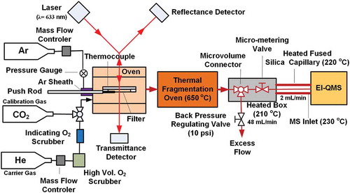
Under normal TOA operation, a particle-laden quartz-fiber filter punch (~ 0.5 cm²) is heated in a sample oven following the IMPROVE_A protocol (Chow et al. 2007). The thermally evolved gaseous products are passed through a manganese dioxide (MnO₂) oxidation reactor, yielding carbon dioxide (CO₂), followed by reduction to methane (CH₄) by hydrogen (H₂) on a nickel (Ni) catalyst. The CH₄ is quantified by a calibrated flame ionization detector (FID). Figure 1 illustrates modifications made to a DRI model 2001 TOA (Atmoslytics, Calabasas, CA) to create the TOA-QMS. To demonstrate feasibility, the MnO₂ and Ni reactors were removed, although when put into practice two parallel streams would be used, as shown by Grabowsky et al. (2011). To reduce air infiltration during sample insertion, the system pressure was increased (from 1.35 × 10⁵ to 1.7 × 10⁵ Pa), and an argon sheath was placed at the interface of the sample pushrod before the oven to reduce O₂ content (from 15.5 to 8.5 ppm). Minimizing O₂ in the ultrapure (99.999%) helium (He) carrier gas reduces the reactions of O₂ with desorbed organic compounds that reduce sensitivity and parent molecule signatures. To minimize condensation of the evolved gases, the microvolume connector and micrometering valve were placed in an enclosed heated box (210°C), connected by a heated (220°C) fused silica capillary to the EI-QMS inlet (230°C). Grabowsky et al. (2011) found that this differential heating reduced the condensation of volatile compounds along the capillary and at the EI-QMS inlet. The QMS flow rate was controlled to ~2 mL min⁻¹ by a micrometering valve.

Figure 1. Schematic of the TOA-QMS system for PM_2.5 organic carbon and inorganic species measurement.

The IMPROVE_A temperature protocol was also simplified for these feasibility tests, as shown in Figure 2a, using 580°C and 840°C temperature steps (with a starting temperature of 80°C), the highest temperatures in the He and He/O₂ carrier gases, respectively, achieved in the protocol. The thermal fragmentation oven obtains molecular fragments similar to those achieved by the widely used Aerodyne Research, Inc. (Billerica, MA), electron impact–aerosol mass spectrometer (EI-AMS) (Jayne et al. 2000) that uses a QMS for detection.

Figure 2. (a) Thermogram from burning of a birch log collected on a quartz-fiber filter comparing the IMPROVE_A temperature protocol with the simplified protocol used with the TOA-QMS; (b) TOA-QMS spectrum obtained for the 580°C portion from m/z 10 to 250, which constitutes most of the evolved gases. Major features are noted at m/z 27, 39, 44, 91, and 115.

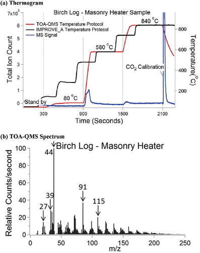
Chemical identification of desorbed molecules was made at 10-min intervals for temperatures of: (1) 80°C to remove water and adsorbed volatile organic compounds (VOCs); (2) 580°C to desorb and pyrolyze molecules from the aerosol deposit; and (3) 840°C to quantify additional compounds that do not evolve at 580°C. A 5% CO₂/95% He mixture was injected as an internal standard using a six-port injection valve with a 1-mL sample loop at the end of each run. The use of CO₂ as the internal standard instead of CH₄ (the original TOA internal standard gas) minimizes interferences between the m/z signals observed from the fragmentation of O₂ (m/z = 16 for O⁺) and CH₄ (m/z = 16 for CH₄⁺). Unit mass resolution is used to quantify NH₄⁺, NO₃⁻, SO₄^2-, and OC, similar to the approach used with the EI-AMS. Figure 2a shows the QMS integrated m/z signal at the different temperatures for a biomass burning sample, with most of the detected signal evolving at 580°C. A mass spectrum of the same sample from m/z 10 to 250 averaged from 900 to 1500 seconds is shown in Figure 2b. Major species are shown with a downward arrow at m/z of 27, 39, 44, 91, and 115. The m/z 27 and 39 signals may represent alkenyl carbocation, while m/z 44 may represent CO₂, C₃H₈, and/or C₂H₄O. Other m/z signals may represent long hydrocarbon chains.

Calibration methods

The EI-AMS calibration approach of Allan et al. (2004) was followed to obtain relative ionization efficiencies (RIE) that relate the mass spectra to chemical concentrations. Weighed amounts of ammonium nitrate (NH₄NO₃) and ammonium sulfate ((NH₄)₂SO₄) were dissolved in distilled-deionized water, while weighed amounts of oxalic acid (C₂H₂O₄, OM/OC = 3.36) were dissolved in isopropanol. C₂H₂O₄ was chosen to represent OC since it is a major primary component of biomass burning (Yang et al. 2009) and is commonly found in atmospheric aerosols (Kerminen et al. 2000). In practice, a broader array of organic compounds would be used, but this single compound is sufficient for feasibility testing. In addition, testing of inorganic compounds containing water-soluble potassium, sodium, and chloride would close the gap needed to analyze samples from current chemical speciation networks. Aerosols were created from these solutions with a constant-output atomizer (TSI, model 3076) fed by a zero-air generator (Environics, model 7000). The solvent associated with the particles was removed by passing the aerosol over activated charcoal for the organics and over silica gel beads for the inorganics prior to being drawn into a Teflon-coated chamber (Chow et al. 1993a) for sampling onto five parallel prefired (~900°C) quartz-fiber filters. Filter flow rates were individually adjusted with mass flowmeters (TSI, model 4043) connected to a vacuum pump to obtain a range of filter loadings. A scanning mobility particle sizer (SMPS) consisting of an electrostatic classifier (TSI, model 3080) and a condensation particle counter (CPC) (TSI, model 3775) measured particle size distributions to estimate filter loading. Filters were stored at 0°C after collection to minimize evaporation losses. Prior to analysis, particle-laden quartz-fiber filters were desiccated for more than 24 hr at 3.5% relative humidity to minimize water content. Evaporative losses during desiccation are expected to be small since samples are still at room temperature, and analysis starts at 80°C. However, further analysis is needed to determine those losses. Portions of the inorganic filters were analyzed by IC for water-soluble ions (Chow and Watson 2017), and a punch (~0.5 cm²) from the organic standards was analyzed by the standard TOA method for OC following the IMPROVE_A protocol (Chow et al. 2007).

Quantitative analysis

Jimenez et al. (2003) outlines the EI-AMS approach to quantifying NH₄⁺, NO₃⁻, SO₄^2-, and OM. A similar approach is adapted for interpreting TOA-QMS spectra. The total number of molecules of a species i, , entering the TOA-QMS is determined from an individual m/z signal as:

(1)

where I_i is the integrated signal (counts) due to species i at the specific m/z over the thermal desorption cycle; X_i is the fraction of the ions from species i that is detected at m/z; and IE_i is the ionization efficiency of species i, equaling the number of ions detected per molecule of the parent species. IE_i is species specific and includes electron ionization efficiency, transmission efficiency from the oven to the detector, the m/z-dependent transmission efficiency of the QMS, and the detection efficiency of the electron multiplier detector.

The mass density of the aerosol deposit for species i, C_i (μg cm⁻²), that produces multiple ions at multiple m/z is:

(2)

where 10⁶ is the conversion factor for μg g⁻¹; MW_i is the molecular weight (g mol⁻¹) of species i; A is the filter punch area (~ 0.5 cm²); N_A is Avogadro’s number (molecules mol⁻¹); and the summation is over all fragment ions (i.e., m/z 1 to n) in the mass spectrum for species i.

The species-dependent IE_i and MW_i are not known for a complex ambient aerosol mixture, but Jimenez et al. (2003) demonstrate that IE_i/MW_i is distinct for inorganics, hydrocarbons, and oxygenated organics, meaning that relative IEs (RIEs) can be used to estimate species mass concentrations. The EI-AMS uses the IE/MW for NO₃⁻ as a reference for the RIEs of NH₄⁺, SO₄^2-and OM. Since the TOA-QMS system has an internal CO₂ calibration for every cycle (see Figure 2a), the CO₂ IE/MW can be used for this purpose. The IE_i/MW_i of any organic and inorganic molecule can be expressed as:

(3)

and C_i can be rewritten to include RIEs:

(4)

where IE_CO2 is the slope of the CO₂ calibration curve (i.e., summed m/z CO₂ signal divided by m/z signal of the calibration peak; see ionization efficiency in Figure 3) for the TOA-QMS. RIEs for NH₄⁺, NO₃⁻, and SO₄^2- are determined by first calculating the slope for individual species (Figure 4) and then calculating the IE/MW ratio to CO₂. For OM or OC, a similar procedure is employed by using data from many species that have been tested, thus calculating an average IE_org/MW_org for hydrocarbons and oxygenated organics. In this feasibility study, only OC was estimated using the C₂H₂O₄ carbon content. OC would be measured separately in a TOA system, so the purpose served here was to determine how well the EI-QMS might reproduce that value.

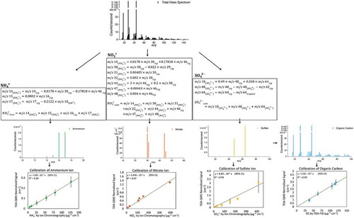
Figure 3. CO₂ ionization efficiency (error bars of ±1 standard deviation derived from replicate analyses are smaller than the size of the dots).

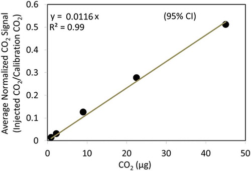
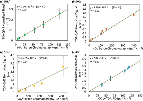
Figure 4. Calibration curves for (a) ammonium, (b) nitrate, (c) sulfate, and (d) organic carbon using oxalic acid (C₂H₂O₄). Error bars indicates ±1 standard deviation derived from replicates. The y-axis shows the corresponding summed species m/z signals from the TOA-QMS normalized using the CO₂ calibration peak m/z signal and divided by the filter punch area in cm². The x-axis values were obtained from quantification by IC and TOA analysis of portions of the filter standards. Linear regression curves are forced through zero.

The partial mass spectrum of species i, , showing the ion contribution from species i at each m/z, is estimated based on a fragmentation table similar to that of the EI-AMS described by Allan et al. (2004). There are important differences between the TOA-QMS and EI-AMS: (1) the particle collection media are quartz-fiber filters in TOA-QMS and a metal cup in EI-AMS; (2) it takes the TOA several seconds to heat the sample to a specified temperature (e.g., 80ºC to 580ºC), while the EI-AMS vaporizer is maintained at a constant temperature (~600ºC) that flash vaporizes nonrefractory PM in <1 msec (Canagaratna et al. 2007); (3) the TOA-QMS vaporizes PM in a pressurized carrier gas (~1.7 × 10⁵ Pa), while the EI-AMS vaporizes PM under vacuum (~10^–5 Pa); (4) the TOA-QMS ionizes the vapors after longer transport time from the TOA to the QMS, while the EI-AMS ionizes the vapors right after vaporization; (5) the TOA-QMS uses He as the carrier gas and EI-AMS typically uses air as the carrier gas; and (6) the TOA-QMS heats samples up to 840°C, higher than in the EI-AMS (~600°C). Therefore, the TOA-QMS is able to analyze data over a more stable and controlled environment, with less interference from external ambient factors. These differences result in similar m/z patterns but different m/z signal magnitudes between the TOA-QMS and EI-AMS. Therefore, while qualitatively similar, the EI-AMS fragmentation tables are not directly applicable to the TOA-QMS. Development of fragmentation tables for the TOA-QMS is the primary focus of this work.

Figure 4 shows the relationship between the TOA-QMS response and the independent IC and TOA measurements. The response curves indicate both reproducibility and linearity for the calibration compounds.

Fragmentation corrections

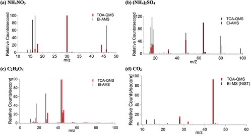
NH₄NO₃, (NH₄)₂SO₄, C₂H₂O₄, and CO₂ mass spectra from the TOA-QMS and EI-AMS are compared in Figure 5, demonstrating the different relative m/z signal intensities. The NH₄NO₃ spectrum (Figure 5a) shows ion peaks at m/z 14 (N⁺), 15 (NH⁺), 16 (NH₂⁺), 17 (NH₃⁺), 18 (NH₄⁺), 30 (NO⁺), and 46 (NO₂⁺). The TOA-QMS also shows CO₂ interference at m/z 44. The (NH₄)₂SO₄ spectrum shows signals at m/z 14 (N⁺), 15 (NH⁺), 16 (NH₂⁺), 17 (NH₃⁺), 18 (NH₄⁺), 32 (S⁺), 48 (SO⁺), and 64 (SO₂⁺). EI-AMS signals at m/z 80 (SO₃⁺), 81 (HSO₃⁺), and 98 (H₂SO₄⁺) in Figure 5b were not detected by the TOA-QMS. The TOA-QMS spectrum for C₂H₂O₄ (Figure 5c) shows major signals at m/z 29, 44, 45, and 46, while the EI-AMS shows major C₂H₂O₄ signals at m/z 17, 27, and 43. Similar mass spectra for CO₂ with ion peaks at m/z 28 and 44 are shown in Figure 5d. These differences in spectra are likely due to inherent difference in the two systems, as discussed in the previous section.

Figure 5. TOA-QMS and EI-AMS spectra for (a) NH₄NO₃, with the most abundant peaks at m/z 14, 15, 16, 17, 18, 30, and 46; (b) (NH₄)₂SO₄, with the most abundant peaks observed at m/z 14, 15, 16, 17, 18, 32, 48, 64, 80, 81, and 98; (c) C₂H₂O₄ with the most abundant peaks for TOA-QMS at m/z 29, 44, 45, and 46, and for EI-AMS at m/z 16, 17, 27, 28, 43, 44, and 45; and (d) CO₂ with the most abundant peak at m/z 44.

NH₄⁺, NO₃⁻, and SO₄^2- mass concentrations were estimated following the format described by Allan et al. (2004) and are presented in the following text, with additional information in Table 1. Most of the m/z signals have contributions from more than one of the major species. NH₄⁺, NO₃⁻, and SO₄^2- become positively charged in the electron impact ionization process and are therefore denoted as NH₄⁺, NO₃⁺, and SO₄⁺. In the following equations, m/z signals labeled with a subscript indicate contributions from the major species to each m/z signal (not the entire m/z signal). The subscript sum denotes the total m/z signal for the species (a sum of all contributing ions or m/z signals), and the subscript sig represents the total m/z signal from all compounds for the specified m/z. The subscript organic is used to denote OC contributions. While simple calibration and measurement of the major species could be performed using just a few of the ions, this work attempts to account for all contributing fragments (m/z signals) to the inorganic species, so that the remainder of the m/z signals can be attributed to OC. This would assume that there are no interferences from other compounds, most of which (e.g., EC and geological minerals) are not expected to decompose in the inert atmosphere. The remaining m/z signal was related to equivalent OC using TOA-FID analysis of C₂H₂O₄ standards.

Table 1. Fragmentation patterns and interference corrections for ammonium, nitrate, and sulfate.

m/z	Ion	Interference ion	Calculation of interference ion	Corrected m/z signal for species
	Ammonium
14	N^+	N^+ (from NO3)	0.0178 × m/z 30 (NO^+→N^+) 0.17818 × m/z 46 (NO2^+→N^+)	Signal at m/z 14, interference fragment
15	NH^+	Organic	Small interference from organic	0.0802 × m/z 16
16	NH2^+	Organic	Small interference from organic	Signal at m/z 16
17	NH3^+	OH^+ (from H2O)	0.2122 × m/z 18	Signal at m/z 17, interference fragment
	Nitrate
14	N^+	Organic	Small interference from organic	0.0178 × signal at m/z 30 + 0.17818 × signal at m/z 46
30	NO^+	Organic at m/z 29	0.022 × m/z 29 (assumed organic)	Signal at m/z 30, interference fragment
31	NO^+	Organic	Small interference from organic	0.00405 × signal at m/z 30
32	NO^+	Organic	Small interference from organic	0.002 × signal at m/z 30
44	N2O^+	Organic at m/z 44	Small interference from organic	2 × signal at m/z 46 + 0.2 × signal at m/z 30
46	NO2^+	Organic	Small interference from organic	Signal at m/z 46
47	NO2^+	Organic	Small interference from organic	0.00443 × signal at m/z 46
48	NO2^+	Organic	Small interference from organic	0.004 × signal at m/z 46
Sulfate
18	Fragment of SO3	H2O	Small interference from organic	0.49 × signal at m/z 48 + 0.268 × signal at m/z 64
48	SO^+	NO2^+	Nitrate at m/z 48 m/z 62 (assumed organic)	Signal at m/z 48, interference fragment
64	SO2^+	Organic	0.5 × m/z 50 (assumed organic) 0.5 × m/z 78 (assumed organic)	Signal at m/z 64, interference fragment

Deconvolution of the ambient mass spectrum begins with removing interferences from the NH₄⁺ spectrum. The total NH₄⁺ signal () is represented as follows:

(5)

where , , and represent the NH₄⁺ contributions to m/z 14, 15, and 17, respectively, while represents the total signal of m/z 16, as it is considered to come entirely from NH₄⁺. Interferences from other compound fragments for m/z 14, 15, and 17 are taken into account as follows:

(6)

(7)

(8)

where (eq 6) is the total m/z 14 signal in the spectrum; the ratios 0.0178 and 0.17818 represent the fractions of m/z 14 generated from the dissociation of NO⁺ (m/z 30) and NO₂⁺ (m/z 46), respectively, for pure NO₃⁺ (see Table 1), while the remainder of the m/z 14 signal represents the dissociation of NH₄⁺ (m/z 18) to N⁺ (m/z 14). The use of these ratios for approximating the contributions from m/z 30 and 46 assumes that organic fragment interferences are minimal (Allan et. al., 2004). The m/z 15 signal (eq 7) results from the fragmentation of NH₂⁺ (m/z 16) into NH⁺ (m/z 15). Therefore, the NH₄⁺ contribution to the m/z 15 signal is found by the ratio of m/z 15 to m/z 16. Since m/z 16 is assumed to be completely from the fragmentation of NH₄⁺ into NH₂⁺, it requires no adjustment for interferences. The m/z 17 signal (eq 8) results from both NH₄⁺ and OH⁺, a fragment of H₂O, which is removed using an m/z 17 to m/z 18 ratio (i.e., 0.2122) from the H₂O spectrum (National Institute of Standards and Technology [NIST] 2014). Elevated H₂O concentrations may introduce higher uncertainties, but this should be minimal, as samples were desiccated and dried in the analyzer at 80°C to reduce H₂O content.

Major NO₃⁺ fragments are found at m/z 30 and 46 signals, constituting 72.75 ± 12.62% of the total NO₃⁺ m/z signal. The total m/z signal, denoted as , is determined as follows:

(9)

where , , , , represent the NO₃⁺ contribution to m/z 14, 30, 31, 32, 44, 47, and 48, respectively. The entire m/z 46 signal is assumed to be due to NO₃⁺ and therefore denoted as . The NO₃⁺ contributions to the remaining m/z signals are determined similar to those for NH₄⁺, using the following equations:

(10)

(11)

(12)

(13)

(14)

(15)

(16)

The NO₃⁺ fraction of m/z 14 is determined from the m/z 14 to m/z 30 and m/z 14 to m/z 46 ratios (i.e., 0.0178 and 0.17818) resulting from the dissociation of NO⁺ and NO₂⁺, respectively (eq 10). A small contribution from organic fragments containing ¹³C affects the m/z 30 signal (eq 11) and is approximated using a fraction of the m/z 29 signal, based upon the m/z 30 to m/z 29 ratio predicted using the International Union of Pure and Applied Chemistry (IUPAC) spectral information (Allan et al. 2004). The NO₃⁺ portions of m/z 31 and m/z 32 are based on pure NO₃⁺ ratios to m/z 30. Separating nitrous oxide (N₂O⁺) from OC at m/z 44 (i.e., m/z 44 could represent CO₂, vinyl alcohol [CH₂CHOH], etc.) is accomplished by finding the fraction of the signal at m/z 44 in relation to m/z 46 and m/z 30 signals (eq 14). The m/z 46 signal is assumed to be completely from the fragmentation of NO₃⁺ into NO₂⁺, and signals at m/z 47 and m/z 48 are fractions of the parent signal at m/z 46 signal based on IUPAC isotopic abundances (eqs 15 and 16). Similar to the EI-AMS, and because only the m/z 30 and 46 signal contributions to the spectrum were used to derive the NO₃⁺ RIE, an adjustment factor that includes the omitted fragments is necessary to correctly estimate the nitrate mass concentration (Hogrefe et al. 2004). An adjustment factor of 1.36 was used for TOA-QMS.

TOA-QMS derived SO₄^2- dominates signals at m/z 18, 48, and 64, which accounts for 77.28 ± 14.48% of the total m/z signal for this species. The total SO₄^2- signal,, is represented by the partial contribution from m/z 18, 48, and 64 signals:

(17)

where , represent the SO₄^2- contribution to m/z 18, 48, and 64, respectively. Identities of the sulfate ion fragments are listed in Table 1. Contributions to m/z 18, 48, and 64 signals are illustrated as follows:

(18)

(19)

(20)

The SO₄^2- signal at m/z 18 signal (eq 18) was calculated using the signal ratios between m/z 18 signal to m/z 48 signal and m/z 18 signal to m/z 64 signal, that is, 0.49 and 0.268, respectively. The SO₄^2- signal at m/z 48 (eq 19) is represented by the signal at m/z 48 minus the interference signals from NO₃⁺ at m/z 48 and an organic contribution estimated as the m/z 62 signal. The SO₄^2- m/z signal at m/z 64 (eq 20) is represented by the signal at m/z 64 minus a fraction of the m/z 50 signal and the m/z 78 signal as:

(21)

While only an approximation of the organics contribution to m/z 64 signal, the signals at m/z 50 and 78 are used since they represent the addition and subtraction of a CH₂ group from a hydrocarbon chain (Allan et al. 2004). Figure 6 shows the process for separating OC from the inorganic species. The OC total m/z signal is calculated by subtracting the sum of the calculated m/z signals of the major inorganic species from the spectrum total m/z signal. C₂H₂O₄ was used to relate the OC total m/z signal to OC mass loading by plotting OC concentration from the C₂H₂O₄-loaded filters using the TOA-FID against the TOA-QMS summed m/z signal of the same C₂H₂O₄-loaded filter. This serves as a calibration curve to estimate total OC in ambient samples (see Figure 4d). OM can be estimated by relating the carbon in C₂H₂O₄ to its molecular weight; however, OM is not reported here as C₂H₂O₄ is highly oxygenated, while the OM/OC multiplier varies by location and time (Turpin and Lim 2001). Further investigation of the spectral data for various organic compounds may offer differentiation between different levels of oxygenated organics, providing the means to better approximate OM and the OM/OC multiplier.

Figure 6. Spectrum processing flow diagram showing how interferences are removed from overlapping m/z signals.

The method detection limit (MDL) for each species is determined by applying the fragmentation table to blank quartz-fiber filters or, in case no signal is detected by the EI-QMS, the y-intercept of the calibration curve. MDLs for NH₄⁺, NO₃⁻, SO₄^2-, and organic carbon equivalent (OCe) species were 1.59, 0.07, 0.96, and 4.22 µg cm⁻², respectively. In comparison, MDLs for ions by IC and for OC by TOA are 0.10 and 0.43 µg cm⁻², respectively. The method may not be as applicable as IC and TOA for samples from pristine environments, but these MDLs are adequate for polluted cities. Different blank filter sets result in slightly different MDLs, and all blank filters (N = 100) were averaged for the MDLs reported in this study.

The higher MDLs of the current method may be a result of several aspects of the instrument: (1) air intrusion and (2) cold spots that may cause condensation of desorbed PM from the quartz-fiber filter. Ambient air may enter the TOA-QMS through the entry port, and further reducing this would reduce oxidation of the ionization filament. While a reduction of cold spots was attempted, some may still be present, causing condensation and further affecting MDLs. More specific heating of the transfer lines, which is possible with a later version of the TOA, could minimize condensation.

A MatLab (MATLAB R2014a, The MathWorks, Inc., Natick, MA) program processed three-dimensional (m/z spectra vs. time) raw data from the QMS by integrating ion currents at each temperature level using the Riemann (1868) sum method. A baseline was determined at each temperature step for each m/z spectrum and subtracted from the sample signal. Integrated m/z signal is normalized using the m/z signal from a CO₂ calibration standard injected at the end of each run. This allows comparison of data from run to run, accounting for slight changes in the system. The m/z signals obtained from TOA-QMS analysis of blank filters are subtracted from sample mass spectral data, and the remaining m/z signals are then deconvoluted into NH₄⁺, NO₃⁻, SO₄^2-, and OC fractions.

The current software removes interferences from ions associated with the ion of interest automatically. The software allows the user to modify and select the fragmentation tables, detection limits, correction factors, and baseline as needed and depending on the properties of the instrument being used. Future software development would include a user interface that allows rapid inspection of the spectra and performance parameters.

Real-world sample analyses

Quartz-fiber filter sample remnants were selected from a refrigerated archive to represent a variety of PM compositions, including: (1) 58 samples with 16 replicates from the Fresno Supersite (Watson et al. 2000); (2) three Fresno samples each from winter, spring, and summer with five replicates (15 total); and (3) 11 samples from near Baltimore, MD (Chen et al. 2002). These samples had been previously analyzed for ions by IC and OC by TOA. Fresno samples contained high NO₃⁻ concentrations, while Baltimore samples contained high SO₄^2- concentrations.

Figure 7 compares the mass loadings of inorganic ions and OC by TOA-QMS with those by IC and TOA analyses. Although reasonable linearity and high correlations were observed for Fresno ions and OC samples (R² = 0.88 to 0.96), and for Baltimore NH₄⁺, SO₄^2-, and OC samples (R² = 0.94 to 0.99), no linearity was found for Baltimore NO₃⁻ samples, likely due to the very low NO₃⁻ levels. Compared to IC analysis of these ambient samples, the TOA-QMS calibrated with the pure compound samples underestimates NO₃⁻ by 24% but overestimates SO₄² by 29%. These deviations are similar to the ±26% reported by the EI-AMS for inorganic measurements when compared with a collocated particle-into-liquid sampler (PILS) (Canagaratna et al. 2007). Discrepancies are possibly due to interference between organic and inorganic signals, or to the formation of different ions as fragmentation occurs. Water-soluble SO₄^2- measured by IC excludes insoluble organosulfates (e.g., ROSO₃) and other insoluble salts (e.g., BaSO₄, PbSO₄, Ag₂SO₄, and SrSO₄) (Hawkins et al. 2010), but these are not expected to be major components found in the atmosphere. The good agreement for NH₄⁺ (slopes of 0.96 for Fresno and 0.85 for Baltimore) indicates that the NO₃⁻ deficit is related to the SO₄^2- surplus, suggesting that a better calibration might be achieved using mixed-salt standards. It also appears from Figure 7 that the lower NO₃⁻ and SO₄^2- concentrations are closer to the 1:1 line than the higher concentrations, indicating that separate calibration curves might be needed for the higher concentrations. The C₂H₂O₄ calibration appears to account well for the OC measured by TOA, which could be a quality control on the TOA when the method is applied in a parallel-stream mode, or possibly even a substitute for the FID.

Figure 7. TOA-QMS concentrations vs. (a) NH₄⁺ by IC, (b) NO₃⁻. by IC, (c) SO₄^2- by IC, and (d) OC by TOA for samples collected in Fresno, CA, and Baltimore, MD. Samples from the western United States, such as those from Fresno, CA, are rich in NO₃⁻, while samples from the eastern United States, such as those from Baltimore, are rich in SO₄^2-.

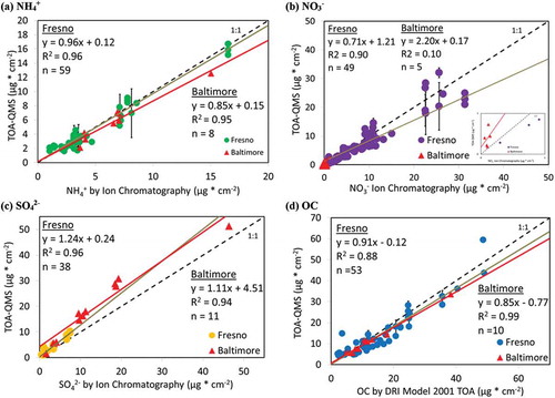
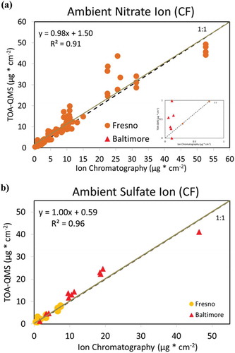
Figure 8 shows that average TOA-QMS derived concentrations can be comparable to those of routine measurements using IC for the 58 Fresno samples. Correction factors (CFs) are sometimes used with EI-AMS measured concentrations to match the concentrations with more established methods (Drewnick et al. 2003; Hogrefe et al. 2004; Jimenez et al., 2003). Using the average ratios of (TOA-QMS)/IC, the CFs are 1.36 for NO₃⁻ and 0.80 for SO₄^2-. After applying these CFs, Figure 9 shows 1:1 comparisons between TOA-QMS and IC measurements with slopes close to unity and high correlations (0.91–0.96).

Figure 8. Average (colored bars) and standard deviations (black lines) of major chemical components in 58 Fresno, CA, samples measured by TOA-QMS, IC, and TOA. Elemental carbon (EC), soil, and salt concentrations determined from TOA, x-ray fluorescence (XRF), and atomic absorption spectrometry (AA), but not by TOA-QMS, are included for completeness. The NO₃⁻ offset is apparent, but the low SO₄^2- averages are in reasonable agreement, as are the NH₄⁺ and OC averages. The soil is calculated using the following formula: Soil = 2.2Al + 2.49Si + 1.63Ca +1.94Ti + 2.42Fe (Malm et al. 1994).

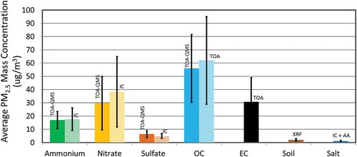
Figure 9. TOA-QMS mass concentration for (a) NO₃⁻ by IC adjusted with a factor of 1.36 plotted vs. IC mass concentration and (b) SO₄^2- by IC adjusted with a factor of 0.80.

Figure 10 presents a time series of PM_2.5 compositions at Fresno corresponding to the 58 samples taken over the period of 12/15/2000 to 2/3/2001 (Chow et al. 2008). Concentrations increased from 12/27/2000 to 1/7/2001 during a prolonged high-pressure system between storms. PM_2.5 NO₃⁻ and OC concentrations during the haze period were elevated, confirming that NO₃⁻ is a large PM_2.5 component, as is well known for winter in central California (Reynolds et al., 2012). Large diurnal variations are also found with elevated NO₃⁻ and OC during the 16:00–24:00 local standard time.

Figure 10. OC and ion contributions to PM_2.5 determined by TOA-QMS at the Fresno Supersite from 12/15/200 to 02/03/2001. Five samples were collected for each day (i.e., 0000–0500, 0500–1000, 1000–1300, 1300–1600, and 1600–2400 local standard time [LST]). Highest concentrations of OC and NO₃⁻ were observed during the late afternoon to night time period (1600–2400 LST).

Summary, conclusion, and future work

This feasibility study demonstrates the possibility of adapting the TOA analysis to obtain major ions, as well as organic carbon from quartz-fiber filter samples, by analyzing the thermally liberated species with an EI-QMS. It is found that spectra similar to those obtained by the EI-AMS can be obtained, but that the ratios of the m/z signals differ and must be remeasured using laboratory-generated standards. Linear relationships are found between QMS signals and prepared standards of NH₄⁺, NO₃⁻, and SO₄^2-. For ambient samples, however, positive deviations are found for SO₄^2-, compensated by negative deviations for NO₃⁻, at higher concentrations. This indicates the possible need to use mixed-compound standards for calibration or separate calibration curves for low and high ion concentrations. The sum of the QMS signals across all m/z after removal of the NH₄⁺, NO₃⁻, and SO₄^2- signals was highly correlated with the carbon content of C₂H₂O₄ standards. For ambient samples, the OC derived from the TOA-QMS method was nearly the same as the OC derived from the standard IMPROVE_A TOA method.

This setup is a practical possibility for the newly designed DRI model 2015 TOA (McGee Scientific, Berkeley, CA). This instrument also allows for simultaneous determination of multiwavelength light absorption and separation of brown carbon from black carbon (Chen et al. 2015; Chow et al., 2015b), as well as providing more precise sample heating that can better bracket the decomposition temperatures of different compounds found in suspended particles (MacKenzie 1970).

Although the feasibility of this approach is evident, there are several issues that need to be resolved in further testing before attempting to adapt TOA to multispecies measurements:

• More experiments are needed to explain why the standardization with pure compounds provided different TOA-QMS responses in real-world samples. This can be explored by using mixtures with different proportions of nitrate and sulfate salts on standards generated by the aerosolization process as described here. Calibrations with more organic compounds are needed to drive more representative RIEs for organic aerosol fractions.

• More experiments are needed to explain why the standardization with pure compounds provided different TOA-QMS responses in real-world samples. This can be explored by using mixtures with different proportions of nitrate and sulfate salts on standards generated by the aerosolization process as described here. Calibrations with more organic compounds are needed to drive more representative RIEs for organic aerosol fractions.

• The EI-QMS portion of the EI-AMS might be a better choice than the generic EI-QMS used for these tests, as this appears to be more optimized for ambient aerosols. Daellenback et al. (2016) and Bozetti et al (2017) have demonstrated the offline use of an AMS by nebulizing water-soluble filter extracts, finding adequate detection limits and good reproducibility. There are also rapid advances in miniature mass spectrometers (Blakeman et al., 2017; Snyder et al., 2016) that may eventually replace the more standard, general-purpose laboratory units. Such a Mini-MS has been demonstrated in a field unit for thermal desorption OC measurements (Cropper, 2016).

• Mass spectra deconvolution methods are continually improving, with much of the improvement motivated by the various AMS versions that are being deployed in source characterization and ambient studies. More advanced approaches that better remove interferences among the aerosol mixture can be incorporated into the TOA-QMS software.

• The parallel sample approach can be implemented in the new model 2015 TOA to add value to the measurements already being acquired in long-term speciation networks with minimal added analysis cost. Even when used with multiple filters accompanied by IC analysis, the single analysis approach would be a useful adjunct.

Acknowledgment

Drs. Glenn Miller of the University of Nevada, Reno, Lung Wen Anthony Chen of the University of Nevada, Las Vegas, and Jerome Robles of the Government of British Columbia, Canada, provided useful suggestions for the experiments and their description.

Additional information

Funding

This research was partially supported by National Science Foundation Grant Nos. 1214163 and 1464501, and the National Park Service IMPROVE Carbon Analysis Contract (C2350000894).

Notes on contributors

Gustavo M. Riggio

Gustavo M. Riggio is a Research Technician at the Desert Research Institute (DRI), Reno, NV, USA.

Judith C. Chow

Judith C. Chow is a DRI Research Professor and an Adjunct Professor at the Institute of Earth Environment, Chinese Academy of Sciences, in Xi’an, People’s Republic of China.

Paul M. Cropper

Paul M. Cropper is a DRI Post-Doctoral Research Fellow.

Xiaoliang Wang

Xiaoliang Wang is a DRI Research Professor.

Reddy L.N. Yatavelli

Reddy L.N. Yatavelli is a Research Engineer at the Air Resources Board, El Monte, CA, USA.

Xufei Yang

Xufei Yang is an Assistant Professor at Montana Tech of the University of Montana, Butte, MT, USA.

John G. Watson

John G. Watson is a DRI Research Professor and an Adjunct Professor at the Institute of Earth Environment, Chinese Academy of Sciences, in Xi’an, People’s Republic of China.

References

- Allan, J.D., A.E. Delia, H. Coe, K. N. Bower, M.R. Alfarra, J.L. Jimenez, A. M. Middlebrook, F. Drewnick, T.B. Onasch, M.R. Canagaratna, J.T. Jayne, and D.R. Worsnop. 2004. A generalised method for the extraction of chemically resolved mass spectra from Aerodyne aerosol mass spectrometer data. J. Aerosol Sci. 35:909–22. doi:10.1016/j.jaerosci.2004.02.007.
- Blakeman, K.H., C.A. Cavanaugh, W.M. Gilliland, and J.M. Ramsey. 2017. High pressure mass spectrometry of volatile organic compounds with ambient air buffer gas. Rapid Commun. Mass Spectrom. 31:27–32. doi:10.1002/rcm.7766.
- Bozzetti, C., Y. Sosedova, M. Xiao, K.R. Daellenbach, V. Ulevicius, V. Dudoitis, G. Mordas, S. Byčenkienė, K. Plauškaitė, et al.. 2017. Argon offline-AMS source apportionment of organic aerosol over yearly cycles for an urban, rural, and marine site in northern Europe. Atmos. Chem. Phys. 17:117–41. doi:10.5194/acp-17-117-2017.
- Canagaratna, M. R., J. T. Jayne, J. L. Jimenez, J. D. Allan, M. R. Alfarra, Q. Zhang, T. B. Onasch, F. Drewnick, H. Coe, A. Middlebrook, et al. 2007. Chemical and microphysical characterization of ambient aerosols with the aerodyne aerosol mass spectrometer. Mass Spectrom. Rev. 26:185–222. doi:10.1002/(ISSN)1098-2787.
- Chen, L.-W.A., J.C. Chow, X.L. Wang, J.A. Robles, B.J. Sumlin, D.H. Lowenthal, R. Zimmermann, and J.G. Watson. 2015. Multi-wavelength optical measurement to enhance thermal/optical analysis for carbonaceous aerosol. Atmos. Measure. Techniques 8:451–61. doi:10.5194/amt-8-451-2015.
- Chen, L.-W.A., J.C. Chow, J.G. Watson, and B.A. Schichtel. 2012. Consistency of long-term elemental carbon trends from thermal and optical measurements in the IMPROVE network. Atmos. Measure. Techniques 5:2329–38. doi:10.5194/amt-5-2329-2012.
- Chen, L.-W.A., B.G. Doddridge, R.R. Dickerson, J.C. Chow, and R.C. Henry. 2002. Origins of fine aerosol mass in the Baltimore–Washington corridor: Implications from observation, factor analysis, and ensemble air parcel back trajectories. Atmos. Environ. 36:4541–54. doi:10.1016/S1352-2310(02)00399-0.
- Chow, J.C. 2015b. Optical calibration and equivalence of a multiwavelength thermal/optical carbon analyzer. Aerosol Air Qual. Res. 15:1145–59. doi:10.4209/aaqr.2015.02.0106.
- Chow, J.C., D.H. Lowenthal, L.-W.A. Chen, X.L. Wang, and J.G. Watson. 2015a. Mass reconstruction methods for PM2.5: A review. Air Qual. Atmos. Health 8:243–63. doi:10.1007/s11869-015-0338-3.
- Chow, J. C., and J. G. Watson. 1999. Ion chromatography in elemental analysis of airborne particles. In Elemental analysis of airborne particles, ed S. Landsberger and M. Creatchman, Vol. 1, 97–137. Amsterdam, The Netherlands: Gordon and Breach Science.
- Chow, J.C., and J.G. Watson. 2013. Chemical analyses of particle filter deposits. In Aerosols handbook: Measurement, dosimetry, and health effects, ed. L. Ruzer, N. H. Harley, and N. York, 179–204. New York, NY: CRC Press/Taylor & Francis.
- Chow, J.C., and J.G. Watson. 2017. Enhanced ion chromatographic speciation of water-soluble PM2.5 to improve aerosol source apportionment. Aerosol Sci. Eng. 1:7–24. doi:10.1007/s41810-017-0002-4.
- Chow, J.C., J.G. Watson, J.L. Bowen, C.A. Frazier, A.W. Gertler, K.K. Fung, D. Landis, and L.L. Ashbaugh. 1993a. A sampling system for reactive speciesin the western United States. In Sampling and analysis of airborne pollutants, ed. E. D. Winegar and L. H. Keith, 209–28. Ann Arbor, MI: Lewis.
- Chow, J.C., J.G. Watson, L.-W.A. Chen, M.-C.O. Chang, N.F. Robinson, D.L. Trimble, and S.D. Kohl. 2007. The IMPROVE_A temperature protocol for thermal/optical carbon analysis: Maintaining consistency with a long-term database. J. Air Waste Manage. Assoc. 57:1014–23. doi:10.3155/1047-3289.57.9.1014.
- Chow, J.C., J.G. Watson, D. H. Lowenthal, K. Park, P. Doraiswamy, K. Bowers, and R. Bode. 2008. Continuous and filter-based measurements of PM2.5 nitrate and sulfate at the Fresno Supersite. Environ. Monit. Assess. 144:179–89. doi:10.1007/s10661-007-9987-5.
- Chow, J.C., J.G. Watson, L.C. Pritchett, W.R. Pierson, C.A. Frazier, and R.G. Purcell. 1993b. The DRI thermal/optical reflectance carbon analysis system: Description, evaluation and applications in U.S. air quality studies. Atmos. Environ. 27A:1185–201. doi:10.1016/0960-1686(93)90245-T.
- Chow, J.C., J.G. Watson, J. Robles, X.L. Wang, L.-W.A. Chen, D.L. Trimble, S.D. Kohl, R.J. Tropp, and K.K. Fung. 2011. Quality assurance and quality control for thermal/optical analysis of aerosol samples for organic and elemental carbon. Anal. Bioanal. Chem. 401:3141–52. doi:10.1007/s00216-011-5103-3.
- Cropper, P.M. 2016. Determination of fine particulate matter composition and development of the organic aerosol monitor. PhD dissertation, Brigham Young University, Provo, UT. http://scholarsarchive.byu.edu/cgi/viewcontent.cgi?article=6667&context=etd (accessed July 31, 2017).
- Daellenbach, K.R., C. Bozzetti, A. Křepelová, F. Canonaco, R. Wolf, P. Zotter, P. Fermo, M. Crippa, J.G. Slowik, Y. Sosedova, et al. 2016. Characterization and source apportionment of organic aerosol using offline aerosol mass spectrometry. Atmos. Measure. Techniques 9:23–39. doi:10.5194/amt-9-23-2016.
- Diab, J., T. Streibel, F. Cavalli, S.C. Lee, H. Saathoff, A. Mamakos, J.C. Chow, L.-W.A. Chen, J.G. Watson, O. Sippula, and R. Zimmermann. 2015. Hyphenation of a EC/OC thermal-optical carbon analyzer to photo ionization time-of-flight mass spectrometry: A new off-line aerosol mass spectrometric approach for characterization of primary and secondary particulate matter. Atmos. Measure. Techniques 8:3337–53. doi:10.5194/amt-8-3337-2015.
- Drewnick, F., J.J. Schwab, O. Hogrefe, S. Peters, L. Husain, D. Diamond, R. Weber, and K.L. Demerjian. 2003. Intercomparison and evaluation of four semi-continuous PM2.5 sulfate instruments. Atmos. Environ. 37:3335–50. doi:10.1016/S1352-2310(03)00351-0.
- Fiore, A.M., V. Naik, and E.M. Leibensperger. 2015. Critical review: Air quality and climate connections. J. Air Waste Manage. Assoc. 65:645–85. doi:10.1080/10962247.2015.1040526.
- Grabowsky, J., T. Streibel, M. Sklorz, J.C. Chow, A. Mamakos, and R. Zimmermann. 2011. Hyphenation of a carbon analyzer to photo-ionization mass spectrometry to unravel the organic composition of particulate matter on a molecular level. Anal. Bioanal. Chem. 401:3153–64. doi:10.1007/s00216-011-5425-1.
- Grahame, T.J., R.J. Klemm, and R.B. Schlesinger. 2014. Public health and components of particulate matter: The changing assessment of black carbon: Critical review. J. Air Waste Manage. Assoc. 64:620–60. doi:10.1080/10962247.2014.912692.
- Hawkins, L.N., L.M. Russell, D.S. Covert, P.K. Quinn, and T.S. Bates. 2010. Carboxylic acids, sulfates, and organosulfates in processed continental organic aerosol over the southeast Pacific Ocean during VOCALS-REx 2008. J. Geophys. Res. 115:D13201. doi:10.1029/2009jd013276.
- Hidy, G.M., P.K. Mueller, S.L. Altshuler, J.C. Chow, and J.G. Watson. 2017. Critical review: Air quality measurements—From rubber bands to tapping the rainbow. J. Air Waste Manage. Assoc. 67:637–68. doi:10.1080/10962247.2017.1308890.
- Hogrefe, O., F. Drewnick, G.G. Lala, J.J. Schwab, and K.L. Demerjian. 2004. Development, operation and applications of an aerosol generation, calibration and research facility. Aerosol Sci. Technol. 38:196–214. doi:10.1080/02786820390229516.
- Jayne, J.T., D.L. Leard, X. Zhang, P. Davidovits, K.A. Smith, C.E. Kolb, and D.R. Worsnop. 2000. Development of an aerosol mass spectrometer for size and composition analysis of submicron particles. Aerosol Sci. Technol. 33:49–70. doi:10.1080/027868200410840.
- Jimenez, J.L., J.T. Jayne. Q. Shi, C.E. Kolb, D.R. Worsnop, I. Yourshaw, J.H. Seinfeld, R.C. Flagan. X. Zhang, K.A. Smith, et al. 2003. Ambient aerosol sampling using the Aerodyne aerosol mass spectrometer. J. Geophys. Res. 108:SOS13-11-SOS13-13. doi:10.1029/2001JD001213.
- Kerminen, V.M., C. Ojanen, T. Pakkanen, R. Hillamo, M. Aurela, and J. Merilainen. 2000. Low-molecular-weight dicarboxylic acids in an urban and rural atmosphere. J. Aerosol Sci. 31:349–62. doi:10.1016/S0021-8502(99)00063-4.
- Lozano, R., M. Naghavi, K. Foreman, S. Lim, K. Shibuya, V. Aboyans, J. Abraham, T. Adair, R. Aggarwal, S.Y. Ahn, et al. 2012. Global and regional mortality from 235 causes of death for 20 age groups in 1990 and 2010: A systematic analysis for the Global Burden of Disease Study 2010. Lancet 380:2095–128. doi:10.1016/S0140-6736(12)61728-0.
- MacKenzie, R.C. 1970. Differential thermal analysis, Vol. 1: Fundamental aspects. New York, NY: Academic Press.
- Malm, W.C., J.F. Sisler, D. Huffman, R.A. Eldred, and T.A. Cahill. 1994. Spatial and seasonal trends in particle concentration and optical extinction in the United States. J. Geophys. Res. 99:1347–70. doi:10.1029/93JD02916.
- Murphy, D.M., J.C. Chow, E.M. Leibensperger, W.C. Malm, M.L. Pitchford, B.A. Schichtel, J.G. Watson, and W.H. White. 2011. Decreases in elemental carbon and fine particle mass in the United States. Atmos. Chem. Phys. 11:4679–86. doi:10.5194/acp-11-4679-2011.
- National Institute of Standards and Technology. 2014. NIST/EPA/NIH mass spectral library (NIST 14) and NIST Mass Spectral Search Program (Version 2.2). Gaithersberg, MD: National Institute of Standards and Technology. https://www.nist.gov/document-3168 (accessed July 31, 2017).
- Pope, C.A., and D.W. Dockery. 2006. Critical review: Health effects of fine particulate air pollution: Lines that connect. J. Air Waste Manage. Assoc. 56:709–42. doi:10.1080/10473289.2006.10464485.
- Reynolds, S., C. Blanchard, D. Lehrman, S. Reid, R. Harley, K. Kleeman, T. Stoeckenius, R. Morris. J.G. Watson, and J.C. Chow. 2012. Synthesis of CCOS and CRPAQS study findings. Fresno, CA: San Joaquin Valley Unified Air Pollution Control District. https://www.researchgate.net/publication/316170523_Synthesis_of_CCOS_and_CRPAQS_study_findings (accessed July 31, 2017).
- Riemann, B. 1868. Über der Begriff eines bestimmten Integrals und den Umfang seiner Gültigkeit. Abhandlungen Der Königlichen Gesellschaft Der Wissenschaften Zu Göttingen 13:87–132.
- Riggio, G.M. 2015. Development and application of thermal/optical- quadrupole TOA-QMS mass spectrometry for quantitative analysis of major particulate matter constituents. MS thesis. University of Nevada, Reno, NV.
- Snyder, D.T., C. J. Pulliam, Z. Ouyang, and R.G. Cooks. 2016. Miniature and fieldable mass spectrometers: Recent advances. Anal. Chem. 88:2–29. doi:10.1021/acs.analchem.5b03070.
- Solomon, P.A., D. Crumpler, J.B. Flanagan, R.K.M. Jayanty, E.E. Rickman, and C.E. McDade. 2014. US national PM2.5 chemical speciation monitoring networks—CSN and IMPROVE: Description of networks. J. Air Waste Manage. Assoc. 64:1410–38. doi:10.1080/10962247.2014.956904.
- Turpin, B.J., and H.J. Lim. 2001. Species contributions to PM2.5 mass concentrations: Revisiting common assumptions for estimating organic mass. Aerosol Sci. Technol. 35:602–10. doi:10.1080/02786820119445.
- Watson, J.G. 2002. Visibility: Science and regulation—2002 Critical review. J. Air Waste Manage. Assoc. 52:628–713. doi:10.1080/10473289.2002.10470813.
- Watson, J.G., J.C. Chow, J.L. Bowen, D.H. Lowenthal, S.V. Hering, P. Ouchida, and W. Oslund. 2000. Air quality measurements from the Fresno Supersite. J. Air Waste Manage. Assoc. 50:1321–34. doi:10.1080/10473289.2000.10464184.
- Watson, J.G., J.C. Chow, G. Engling, L.-W.A. Chen, and X.L. Wang. 2016. Source apportionment: Principles and methods. In Airborne particulate matter: Sources, atmospheric processes and health, ed. R.M. Harrison, 72–125. London, UK: Royal Society of Chemistry.
- Watson, J.G., J.C. Chow, and C.A. Frazier. 1999. X-ray fluorescence analysis of ambient air samples. In Elemental analysis of airborne particles, ed. S. Landsberger and M. Creatchman, Vol. 1, 67–96. Amsterdam, The Netherlands: Gordon and Breach Science.
- Watson, J.G., R.J. Tropp, S.D. Kohl, X.L. Wang, and J.C. Chow. 2017. Filter processing and gravimetric analysis for suspended particulate matter samples. Aerosol Sci. Eng. 1:193–205. doi:10.1007/s41810-017-0010-4.
- Yang, F., H. Chen, X.N. Wang, X. Yang, J.F. Du, and J.M. Chen. 2009. Single particle mass spectrometry of oxalic acid in ambient aerosols in Shanghai: Mixing state and formation mechanism. Atmos. Environ. 43:3876–82. doi:10.1016/j.atmosenv.2009.05.002.