Development of visibility forecasting modeling framework for the Lower Fraser Valley of British Columbia using Canada’s Regional Air Quality Deterministic Prediction System

ABSTRACT

Visibility degradation, one of the most noticeable indicators of poor air quality, can occur despite relatively low levels of particulate matter when the risk to human health is low. The availability of timely and reliable visibility forecasts can provide a more comprehensive understanding of the anticipated air quality conditions to better inform local jurisdictions and the public. This paper describes the development of a visibility forecasting modeling framework, which leverages the existing air quality and meteorological forecasts from Canada’s operational Regional Air Quality Deterministic Prediction System (RAQDPS) for the Lower Fraser Valley of British Columbia. A baseline model (GM-IMPROVE) was constructed using the revised IMPROVE algorithm based on unprocessed forecasts from the RAQDPS. Three additional prototypes (UMOS-HYB, GM-MLR, GM-RF) were also developed and assessed for forecast performance of up to 48 hr lead time during various air quality and meteorological conditions. Forecast performance was assessed by examining their ability to provide both numerical and categorical forecasts in the form of 1-hr total extinction and Visual Air Quality Ratings (VAQR), respectively. While GM-IMPROVE generally overestimated extinction more than twofold, it had skill in forecasting the relative species contribution to visibility impairment, including ammonium sulfate and ammonium nitrate. Both statistical prototypes, GM-MLR and GM-RF, performed well in forecasting 1-hr extinction during daylight hours, with correlation coefficients (R) ranging from 0.59 to 0.77. UMOS-HYB, a prototype based on postprocessed air quality forecasts without additional statistical modeling, provided reasonable forecasts during most daylight hours. In terms of categorical forecasts, the best prototype was approximately 75 to 87% correct, when forecasting for a condensed three-category VAQR. A case study, focusing on a poor visual air quality yet low Air Quality Health Index episode, illustrated that the statistical prototypes were able to provide timely and skillful visibility forecasts with lead time up to 48 hr.

Implications: This study describes the development of a visibility forecasting modeling framework, which leverages the existing air quality and meteorological forecasts from Canada’s operational Regional Air Quality Deterministic Prediction System. The main applications include tourism and recreation planning, input into air quality management programs, and educational outreach. Visibility forecasts, when supplemented with the existing air quality and health based forecasts, can assist jurisdictions to anticipate the visual air quality impacts as perceived by the public, which can potentially assist in formulating the appropriate air quality bulletins and recommendations.

Introduction

Visibility impairment, due to atmospheric particulate matter and gases, is one of the most noticeable indicators of air pollution and is a concern in many urban cities, as well as national parks and wilderness areas. While the ecological and human health effects of air pollution have traditionally been considered of primary importance, the impacts of air pollution on visibility, also known as visual air quality, continue to be an emerging field of interest for the scientific research community, governing bodies, and the public. In the past decade, there has been a growing amount of visibility-related research, including (1) characterization studies, which examined the various spatial and temporal patterns and source contributions to visibility impairment (Brewer and Moore 2009; Mölders and Gende 2015; So et al. 2014; Wan et al. 2011), (2) observational studies, including the assessment and development of monitoring methods and techniques (Arnott et al. 2005; Chen et al. 2013; Gao et al. 2007; Lin and Li 2016; Moosmüller, Chakrabarty, and Arnott 2009), and (3) scenario modeling work that investigated the potential impacts of changing emissions and climate on visibility (British Columbia Visibility Coordinating Committee[BCVCC] 2017a; RWDI 2006; So et al. 2014). Due to increased willingness of the general public to participate in scientific research and the rise in network technology, there have been a number of visibility-related citizen science projects (Dolan 2016; Poduri, Nimkar, and Sukhatme 2010; Snik et al. 2014), which have transformed scientific data collection where a network of users can increase both spatial and temporal coverage of the existing ground-based measurement network. In addition to the U.S. Regional Haze Rule (U.S. Environmental Protection Agency 1999), which protects visibility in national parks and wilderness areas across the United States, the need to protect urban visual air quality has been recognized in a number of local jurisdictions in North America (Arizona Department of Environmental Quality 2003; BCVCC 2015a; Ely et al. 1991).

In the Lower Fraser Valley (LFV) of British Columbia (BC), Canada, a region with mountainous vistas and scenic views, visual air quality can become impaired when PM_2.5 concentrations are as low as 8 to 9 µg/m³ and can be severely degraded when concentrations rise above 20 µg/m³ based on two field campaigns, REVEAL I and REVEAL II (Pryor and Barthelmie 2000; Pryor et al. 1997), conducted in the mid 1990s. Studies have indicated that visibility impairment in the LFV can negatively impact on a number of key local economic sectors such as tourism, film, and real estate industries. Based on tourist surveys conducted in 1999, a single poor visibility event in the LFV could result in revenue losses of up to $9 million (McNeill and Roberge 2000). As BC tourism revenues doubled between 1999 and 2009, it is estimated that future revenue losses, based on three distinct poor visibility events per year, could reach up to $55 million per year (BCVCC 2015b). Other studies have illustrated that poor visual air quality conditions can diminish the quality of life for residents (Furberg and Preston 2005; Haider et al. 2002), can affect the yield of crops and productivity of natural ecosystems through the attenuation of photosynthetically available radiation (Chameides et al. 1999; Grantz, Garner, and Johnson 2003), and can disrupt the flow of knowledge transfer for Aboriginal people (Carlson 2009) in the LFV.

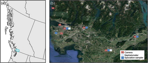
The British Columbia Visibility Coordinating Committee (BCVCC), a joint initiative between regional, provincial, and federal air quality agencies, was established in 2006 with a vision to achieve clean air and pristine visibility for the health and enjoyment of present and future generations in BC. Since 2010, the BCVCC has undertaken a pilot project to develop a visual air quality management plan for the LFV within a framework that can be applicable elsewhere in BC and Canada. A dedicated multi-instrumented visual air quality monitoring network (Figure 1) was integrated into the larger LFV Air Quality Monitoring Network (Metro Vancouver 2015). This network, as of 2017, employs 10 digital cameras and five nephelometers to track visibility conditions and to report a Visual Air Quality Rating (VAQR; Kellerhals 2016). The VAQR is reported as a five-category index during daylight hours, when relative humidity (RH) is less than or equal to 75%: “excellent” (< 11 dv), “good” (11–16.5 dv), “fair” (16.5–22 dv), “poor” (22–27.5 dv), and “very poor” (> 27.5 dv), where the deciview (dv) thresholds were established by a local perception study (Gallagher and McKendry 2011). Visual air quality data collected from this network have been analyzed in wildfire smoke impact studies and characterization studies (So et al. 2014) to increase our understanding of aerosol contributions to visual air quality impairment in the LFV. Both the VAQR and camera images are available near real-time to the public through the Clear Air BC website (BCVCC 2017b). In this paper, we explore the next step in visual air quality reporting, which is providing visibility forecasts in relation to air quality conditions to the public.

Figure 1. Visual air quality monitoring network in the Lower Fraser Valley of British Columbia as of 2017. The shaded region in (a) highlights the geographical location of the monitoring network (b) in southwestern British Columbia.

Visibility forecasts, when timely and reliable, can play an important role as part of the air quality management plan, working in concert with the more traditional air quality and health-based forecasts. The main applications of visibility forecasts fall into the following broad categories including: tourism and recreation planning, supplementation of visual air quality management programs, educational outreach, and providing guidance during poor air quality episodes. As tourism is a major source of revenue in the LFV, where scenic vistas are highly valued by residents and visitors alike, visibility forecasts can provide useful information to the public and tour operators when planning for wilderness and scenic experience activities. Timely and reliable visibility forecasts, when available, can supplement existing visual air quality management programs, where on days with poor visibility forecasts, jurisdictions can recommend practical ways to reduce emissions, which can benefit both PM_2.5 reduction and visibility improvement efforts. These forecasts can also serve as an educational outreach tool to inform the public regarding the visual and health impacts of poor air quality. During poor air quality episodes, visibility forecasts can assist jurisdictions to anticipate the visual air quality impacts as perceived by the public, which can potentially assist in formulating the appropriate air quality bulletins and recommendations. To the best of our knowledge, issuing visibility forecasts during daylight hours, for visual air quality management and non-aviation-related recreational purposes, is a novel concept and has not been implemented elsewhere in North America. As a specialized experimental product, we introduce a set of new prototype methods to forecast visibility conditions by leveraging the available air quality and meteorological forecasts from Canada’s operational air quality forecast system. The end product, in the form of comprehensive, reliable, and timely visibility forecasts, can provide an added benefit to air quality agencies, as well as to the public, and can inform both air quality and visibility management in impacted airsheds.

Background

Visibility impairment is commonly quantified by the light extinction coefficient, which is defined as the fractional loss of image-forming light per unit distance due to scattering and absorption by particles and gases in the atmosphere. Light extinction can be measured using a long path transmissometer or reconstructed using optical point and absorption measurements. Alternatively, extinction can also be reconstructed using 24-hr visibility-degrading aerosol concentrations according to the revised IMPROVE algorithm (Pitchford et al. 2007), which describes the effects of particulate composition, particle size distribution, and hygroscopic growth on visibility degradation (Lowenthal and Kumar 2006; Malm et al. 2003; Malm and Hand 2007; Tang, Tridico, and Fung 1997), as shown in eq 1:

(1)

for

for

where f_s (RH) and f_L (RH) are water growth functions for small and large size mode sulfate and nitrate components, respectively; f_ss(RH) is the water growth function for sea salt particles; [AS], [AN], [OM], [EC], [FS], and [SS] are the concentrations (µg/m³) of ammonium sulfate, ammonium nitrate, organic matter, elemental carbon, fine soil, and sea salt, respectively; and X = [AS], [AN], or [OM] mass concentrations depending on the term.

In an effort to provide time-resolved extinction while using U.S Environmental Protection Agency (EPA) standard monitoring methods, a hybrid method (Pitchford 2010) was developed to estimate hourly light extinction due to PM_2.5 based solely on ambient hourly PM_2.5 concentrations, relative humidity (RH), and monthly average historical PM_2.5 species composition. The hybrid method is based on the original IMPROVE algorithm (Lowenthal and Kumar 2003), where a single particle dry-mass light extinction efficiency and water growth factor is applied regardless of the particle size for sulfate, nitrate, and organic mass. The inherent differences between the revised and original IMPROVE algorithm are described in detail in Pitchford et al. (2007). This method was later extended (So et al. 2015) to provide total light extinction by incorporating the scattering effects of coarse mass and the scattering and absorption effects of gases as per the revised IMPROVE algorithm. The extended hybrid model can be summarized as

(2)

where

and

where f(RH) is the water growth function used in the original IMPROVE algorithm (Lowenthal and Kumar 2003), HF denotes the hygroscopic fraction, DLEE refers to dry-mass light extinction efficiency, [AS], [AN], [OM], [EC], and [FS] are the concentrations (µg/m³) of ammonium sulfate, ammonium nitrate, organic matter, elemental carbon, and fine soil, respectively, and CMtoSUM_ratio is the monthly averaged [CM] to [SUM] ratio based on historical speciation data. Details on the computation and formulas used to reconstruct PM_2.5 and coarse mass can be found in So et al. (2015). Note that Rayleigh scattering is set to 13.2 Mm⁻¹ in this study, to correspond with the nephelometer readings centered at a wavelength of 530 nm. Results from So et al. (2015) indicated that the extended hybrid method can provide relatively accurate and time-resolved estimates of extinction at sites with or without site-specific speciation profile in the LFV. Both the revised IMPROVE algorithm and the extended hybrid method were considered in this study when developing the visibility forecasting prototypes.

Methods

Study sites

This study was conducted using air quality and meteorological forecasts and observations and visibility-related measurements collected at three air quality monitoring stations located within the LFV of BC (Figure 1). All three sites are part of the LFV Air Quality Monitoring Network (Metro Vancouver 2015), as well as the National Air Pollution Surveillance Network (NAPS; Dabek-Zlotorzynska et al. 2011), and are operated by Metro Vancouver. From west to east, the study sites include Vancouver Airport (YVR), Burnaby South (BBY), and Chilliwack Airport (YCW). The Vancouver Airport site (YVR) is located in an urbanized area at the Vancouver International Airport (49.186 ºN, 123.153 ºW). Notable sources of emissions include industrial, vehicular, emissions from aircraft and airport operations, and wood-smoke emissions from nearby residential areas during the cold seasons. The Burnaby South site (BBY) is located in an urban-residential area (49.216 ºN, 122.983 ºW) and is surrounded by lands with diverse land uses, including industrial, residential, and conservation areas. The Chilliwack Airport site (YCW) is located further east at the Chilliwack Municipal Airport (49.156 ºN, 121.941 ºW) in a residential neighborhood surrounded by agricultural land from the northeast to west. Detailed information for each station, such as land use, terrain, and surrounding population density, can be found in Metro Vancouver (2012).

Data sources

LFV Air Quality Monitoring Network

Optical point scattering and absorption measurements were used to reconstruct 1-hr total extinction for various periods from 2010 to 2012. The Optec NGN-2a Open Air Integrating Nephelometer with light-emitting diode (LED) light source was used to measure continuous 1-hr light scattering coefficient due to particles and gases at a wavelength centered at 530 nm. The nephelometer outputs raw data in terms of “light counts,” and postprocessing of these raw data using clean air and calibration gas readings is required to calculate the scattering coefficient via a linear calibration equation (Optec, Inc. 2006). Details on the theory of operation and operating procedures can be found in Optec, Inc (2006). NO₂ and black carbon measurements were used to estimate the light absorption by gases and particles and were attained by the Thermo Scientific Model 17C NH₃/NO_x Analyzer and the Magee Scientific AE-22 Aethalometer, respectively. The 1-hr optical reconstructed extinction values, along with the corresponding VAQR, were used to evaluate model forecast performance. Digital images captured by the co-located cameras were used to confirm visual air quality impacts.

National Air Pollution Surveillance Network

Integrated 24-hr ambient aerosol particle sample, collected using collocated Thermo Scientific samplers (Partisol-Plus 2025-D sequential dichotomous particulate sampler and the Partisol model 2300 sequential speciation sampler), were used to establish historical PM speciation profiles and to reconstruct 24-hr extinction using the revised IMPROVE algorithm (Pitchford et al. 2007). It should be noted that BBY was the only site that had co-located speciation measurements. PM speciation samples collected at BBY and Abbotsford Airport were used to construct historical PM speciation profiles for YVR and YCW, respectively. Model forecast assessment for aerosol extinction attribution was conducted at BBY only. All PM speciation samples are analyzed by the Analysis and Air Quality Section (AAQS) of Environment and Climate Change Canada in Ottawa in accordance with the National Air Pollution Surveillance Network (NAPS) PM_2.5 speciation program. Details of the sampling and analytical methods, as well as the formulas used for mass reconstruction of major aerosol chemical components, can be found in Dabek-Zlotorzynska et al. (2011).

Regional Air Quality Deterministic Prediction System

The RAQDPS is the operational air quality forecasting system at Environment and Climate Change Canada and consists of a number of components, including a regional air quality model (GEM-MACH) and a number of postprocessing suites and packages. The RAQDPS uses GEM-MACH (Global Environmental Multiscale—Modeling air quality and chemistry; Moran et al. 2010; 2011; Makar et al. 2015; Makar et al. 2014) to comprehensively model air quality using a full description of atmospheric chemistry and meteorological processes (Anselmo et al. 2010). GEM-MACH is an online, one-way coupled chemical transport model embedded within the Global Environmental Multiscale numerical weather prediction model. During majority of the study period, GEM-MACH (v1.4.5 and v1.4.6) operated on a 15-km horizontal grid and 58 vertical levels extending up to 0.1 hPa over a North American domain (Moran et al. 2011) and was later changed to a 10-km grid and 80 vertical levels following an update (v1.5.0) on October 2, 2012. GEM-MACH employs a simple two-bin sectional representation of the PM size distribution (0–2.5 µm and 2.5–10 µm) and considers nine chemical components, including SO₄, NO₃, NH₄, elemental carbon, primary and secondary organic aerosol, crustal material, sea salt, and particle-bound water (Moran et al. 2011). GEM-MACH provides 48-hr forecasts twice daily (at 00:00 and 12:00 UTC) of hourly surface concentrations of O₃, NO₂, particulate matter (PM), and other chemical components on a North American grid. As part of the RAQDPS, a statistical postprocessing package (UMOS-AQ; Wilson and Vailée 2002) is applied to the raw hourly forecasts to reduce model bias and model error at point locations with air quality monitors using a multiple linear regression approach. These values are then assimilated into RAQDPS forecasts and are used as primary guidance from which the operational meteorologists generate public Air Quality Health Index (AQHI; Stieb et al. 2008) forecasts. UMOS-AQ combines multiple sources of information including air quality and meteorological forecasts, air quality measurements, and physical variables. Verification analyses have indicated that UMOS-AQ has shown significant improvements over the raw GEM-MACH forecasts in both the summer and winter seasons and can provide high-quality national guidance in air quality forecasting (Antonopoulos et al. 2011). This study considered both the historical observations and numerical data and forecasts that were available through the RAQDPS as predictor variables when forecasting visibility conditions.

The observational air quality data extracted as part of UMOS-AQ were from automated near real-time hourly reports of O₃, PM_2.5, and NO₂ from NAPS air quality stations across Canada. It should be noted that these data had not been fully verified at this point and may not be representative of the observed conditions. In this study, these observational data were postprocessed by PROGNOS (Teakles et al. 2017a), an experimental postprocessing system that is currently under development, to generate persistence and antecedent predictors when constructing the visibility forecasting prototypes. PROGNOS is an initiative at ECCC to renew the operational statistical postprocessing infrastructure, which will better accommodate the evolving meteorological and air quality forecast program requirements. Persistence predictors are observed air quality pollutant concentrations at the time when the air quality model is initiated. Antecedent predictors, which are not currently available through the RAQDPS, are the maximum, minimum, and observed air quality pollutant concentrations at the same local hour as the forecast, within a 24-hr period prior to model initiation. Numerical data from an air quality forecast model, GEM-MACH (v1.4.5; v1.4.6; v1.5.0), were used to produce direct and calculated predictor variables. These predictors included meteorological variables (model dry bulb temperature, wind component, geopotential height, relative humidity, dew-point depression, surface model pressure, cumulative precipitation, average rate of snowfall in water equivalent, cloud cover, model boundary-layer height, wind speed, and dew-point temperature), chemical variables (the maximum and average O₃, PM_2.5, and NO₂ concentrations during 3-, 6-, and 24-hr intervals), and other predictor variables listed by UMOS-AQ as physical variables (the downward solar flux, calculated mixing height, day of week, and sine of Julian day) (Peng et al. 2017). Both the unprocessed (GEM-MACH) and UMOS-AQ postprocessed air quality forecasts were considered, although not simultaneously, as predictor variables when constructing visibility forecast models.

Model building process overview

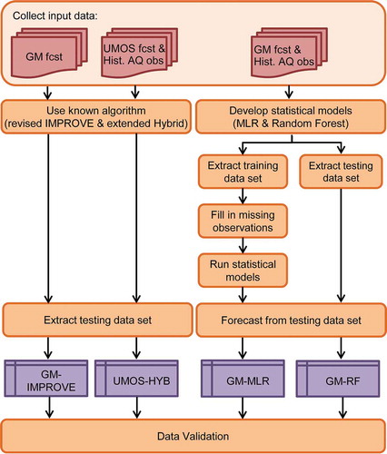
An overview of the visibility forecasting model building and validation framework is illustrated in Figure 2. The input data used in developing the baseline model and various prototypes included historical observations from the air quality and visual air quality network and physical variables, and numerical forecasts such as air quality and meteorological fields from the RAQDPS. Using various combinations of air quality forecasts (GEM-MACH and UMOS-AQ) and PM speciation profiles (GEM-MACH and historical), four visibility forecasting models (GM-IMPROVE, UMOS-HYB, GM-MLR, and GM-RF) were generated using known algorithms such as the revised IMPROVE algorithm (Pitchford et al. 2007) and the extended hybrid method (So et al. 2015), and through training and applying statistical regression models such as multiple linear regression (MLR) and random forest (RF). Details on the individual model inputs and configurations are illustrated in Table 1. Of the four models, GM-IMPROVE serves as the baseline model, and translates the raw GEM-MACH air quality forecasts into visibility forecasts using the revised IMPROVE algorithm. UMOS-HYB is a model that uses the postprocessed air quality forecasts and historical PM speciation profile to forecast visibility using the extended hybrid approach. No additional statistical training is required for both of these models, and they can be relatively easy to implement within the current infrastructure. GM-MLR and GM-RF are the statistical prototypes, where the raw GEM-MACH air quality forecasts, along with other meteorological, chemical, and physical variables, are used as inputs to train both a linear (multiple linear regression, MLR) and a nonlinear (random forest, RF) statistical model, respectively, to forecast visibility. The MLR approach was selected as the linear model as it is currently employed by UMOS-AQ to postprocess air quality forecasts. For the nonlinear model, the RF approach was selected as it is a nonparametric modeling technique that has relatively strong predictive performance across many subject domains. RF models can utilize the same inputs as MLR without additional data processing or model tuning, and provide a measure of variable importance implicitly, which can also be used to examine variable interactions. Model training was performed using data prior to 2012, with various start dates depending on data availability at each site (YVR: February 11, 2011; BBY: June 21, 2011; YCW: July 1, 2010). Missing extinction observations in the training data set were filled with synthetic values estimated using the extended hybrid method based on observed PM_2.5 and RH when available. This step was especially important at YVR as approximately 25% of the training data was substituted with synthetic values. Data availability at BBY and YCW were higher, where only 2 and 7% of the training set consisted of synthetic data, respectively. Model development was undertaken using R version 3.2.3, in particular through the use of two statistical packages, leaps (Lumley, 2009) and randomForest (Liaw and Wiener 2012). The leaps package was used for predictor selection when conducting MLR and the randomForest package was used to create random forest regression models for the GM-RF prototype. Testing and validation was conducted using a separate data set, all available 2012 data from January 1 to October 31, 2012, without any data substitution for missing data. Model performance was assessed by comparing the forecasts with both 1-hr optical and 24-hr aerosol reconstructed extinction, as well as the observed VAQR.

Table 1. Model inputs and configuration for the visibility forecasting models.

Model	AQ forecast	PM speciation profile	Algorithm
GM-IMPROVE	GEM-MACH	GEM-MACH	Revised IMPROVE
UMOS-HYB	UMOS-AQ	Historical	Extended hybrid
GM-MLR	GEM-MACH	GEM-MACH	MLR
GM-RF	GEM-MACH	GEM-MACH	RF

Figure 2. Visibility forecasting model building and validation framework.

Data preprocessing

A set of quality control filters was applied to ensure that both the training and testing data sets consisted of high-quality data that were both reasonable and representative of visibility impairment due to air pollution in the LFV. Cases with RH greater than 90% were not analyzed in this study, as these cases were likely affected by weather events such as fog or precipitation. Cases where the 1-hr optical reconstructed extinction was greater than 300 Mm⁻¹ were first validated with digital camera images to confirm visibility impairment and were consequently scaled down to 300 Mm⁻¹ due to uncertainty in the accuracy and precision of the instrument beyond this threshold. These cases occurred less than 0.5% in both the training and testing data sets. Although the hourly extinction values may not be as accurate, these cases were retained as they illustrate the rare occurrences of “poor” or worse visibility conditions in the LFV. Additional analyses were conducted to ensure that the observed PM_2.5 and extinction were consistent with one another. Cases with hourly PM_2.5 < 1.5 µg/m³ had to be in the “good” or better VAQR (≤ 52.1 Mm⁻¹), and cases with hourly PM_2.5 > 15 µg/m³ had to be in the “poor” or worse VAQR (≥ 90.3 Mm⁻¹). In total, 734 cases (2% of all available data with RH less than or equal to 90%) were excluded due to this consistency filter. Cases affected by forest fire smoke, such as the 2012 Siberian forest fire (Teakles et al. 2017b), were also excluded as the air quality model did not include transpacific and regional forest fire emissions during the study period. These cases were identified by analyzing the location of the smoke plumes based on Hazard Mapping System Fire and Smoke analysis (National Oceanic and Atmospheric Administration [NOAA] 2017).

Statistical methods

Multiple linear regression (MLR)

MLR is a linear regression method, where the response variable is expressed as a linear combination of two or more predictor variables. In this study, 97 predictor variables, with at least 90% data availability, were considered when constructing the individual MLR models for each forecast hour by site, regardless of model initialization time (00:00 and 12:00 UTC). Using the leaps package in R, the sequential replacement algorithm (Miller 2002) was used to identify the best subset of variables for each model size from 1 to a default maximum of 25 predictors. Compared with the stepwise forward or backward variable selection approach, the sequential replacement algorithm is found to be more comprehensive and is less computationally intensive and time-consuming than performing an exhaustive search, when considering a large number of variables (Miller 2002). The final, most optimal, subset of predictors for each MLR model from the 25 candidate models was selected by minimizing the Bayesian information criterion (BIC), while ensuring that the best selected model had at least a 1% improvement over the previous model size. In general, the final MLR models often had less than 10 predictors, where the most commonly selected variables included PM_2.5 concentrations 24 hr prior to model initiation (a persistent variable), the minimum PM_2.5 concentrations within a 24-hr period prior to model initiation (an antecedent predictor), sine of Julian day (a physical predictor), modeled dry bulb temperature at the surface (a meteorological predictor), and the spatial average of PM_2.5 concentrations from GEM-MACH for lower levels (below 850 HPa height) calculated from the last 3 and 6 hr (a chemical predictor).

Random forests (RF)

In RF regressions, a nonparametric ensemble modeling approach is adopted by employing the bootstrap aggregation (bagging) technique (Breiman 1996), where an ensemble of regression trees is derived by using random subsets of the data and a subset of randomly chosen predictors to determine the split at each node (Liaw and Wiener 2002). The randomForest package in R, which uses the Fortran implementation of the random forest algorithm by Breiman and Cutler (2004), was used to construct a machine learning-based visibility forecasting model, where the number of trees was set to 500 and one-third of the available 97 predictor variables were randomly selected for splitting at each node until five or fewer cases remain in the terminal node. The RF predictor is formed by taking the average prediction from all the trees in the forest. As the number of trees in the forest becomes large, the prediction error for random forests converges to a limit (Breiman 2001). RF can process up to thousands of predictors quickly and can automatically fit highly nonlinear interactions. Studies showed that RF is robust against overfitting when applied to noisy data (Díaz-Uriarte and Alvarez De Andrés 2006; Ziegler and König 2014; Matsuki, Kuperman, and Van Dyke 2016) and performs well compared with other machine learning methods, including support vector machines, neural networks, and adaptive boosting (Díaz-Uriarte and Alvarez De Andrés 2006; Liu et al. 2013; Ogutu, Piepho, and Schulz-Streeck 2011).

Model assessment

To assess model performance in forecasting 1-hr extinction values, a number of statistical scores, including the Pearson’s correlation coefficient (R), normalized mean bias (NMB), and normalized mean error (NME), were computed and compared between the different models under a variety of meteorological and visual air quality conditions, with a stronger focus on daylight conditions when visibility degradation is more prominent. Daylight hours are defined as those that fall between and including 2 hr after and before the daily sunrise and sunset time in Vancouver, respectively. Details on the individual statistical scores and their associated ranges and perfect score can be found in the appendix. In the case of VAQR categorical forecast, the proportion correct (PC), Heidke Skill Score (HSS; Heidke 1926), and the hit rate and false alarm ratio for the “poor” or worse categories were used to assess forecast performance. These statistics have been widely used in assessing categorical weather forecasts (Jolliffe and Stephenson 2012; JWGFVR 2009; Kluepfel 2004; Zhang and Casey 2000), and the computational details can be found in the appendix.

Results and discussion

Aerosol reconstructed extinction

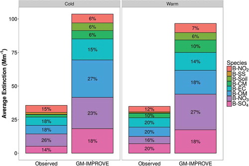
Figure 3 illustrates the average extinction contribution by particles and gases during cold and warm months for the observed and baseline model (GM-IMPROVE) at Burnaby South (BBY). The GM-IMPROVE forecast was generated using the revised IMPROVE algorithm based on the raw GEM-MACH air quality and relative humidity forecasts from the RAQDPS. Although GM-IMPROVE overestimated total extinction more than twofold, the relative contributions to visibility impairment from most species, including the major components of PM such as ammonium sulfates, ammonium nitrates, organic mass, and elemental carbon, were similar to those of the observed. This large discrepancy in total extinction was mainly due to an overestimation of PM species by GEM-MACH and, to a lesser degree, higher relative humidity forecasts, which also inflated their contributions (not shown). It should be noted that GM-IMPROVE did not estimate sea salt contributions, as sea salt measurements were not readily available from the RAQDPS, when the data sets were extracted for this study. No further efforts were employed to estimate sea salt contributions as they did not significantly contribute to the total extinction loss in the LFV (So et al. 2014). The relative contributions from fine soil were largely overestimated during both seasons, which may be due to errors in the emission inventory or the lack of meteorological modulation of fugitive dust emissions, where the suppression effects of meteorological conditions such as snow cover or recent precipitation on surface fugitive dust were unaccounted for (Moran et al. 2011, 2012). During the colder months, the relative contributions from ammonium sulfate and ammonium nitrate were forecast well by GM-IMPROVE, with less than 5% deviation from the observed. Percent contributions from organic mass were overestimated by approximately 10%, which may be indicative of errors in wintertime wood-smoke emissions. NO₂ relative contributions were also underestimated by approximately 10%. For ammonium sulfate and ammonium nitrate, the extinction attribution forecasts during the warmer months were similar to those of colder months, which suggests that the model did not fully capture the known seasonal variation for these species. Higher ammonium sulfate is observed during summertime in the LFV due to increased rates of photochemical conversion of SO₂ to sulfate and increased biogenic sulfur emissions. Ammonium nitrates tend to be higher during wintertime due to increase in nitrate particle formation during cooler temperatures and higher humidity. The relative contributions from organic mass and coarse mass during the warmer months were forecast well by GM-IMPROVE. Overall, these results indicated that the baseline model, GM-IMPROVE, had skill in forecasting the relative species contributions to visibility impairment.

Figure 3. The average observed and GM-IMPROVE forecast 24-hr extinction contribution by particle and gases during cold (January to March; October to December) and warm months (April to September) at Burnaby South. Forecast values were based on GEM-MACH 12:00 UTC run for forecast hours 25 to 48. The relative observed extinction contribution from soil and sea salt was 1% and 2%, respectively, during both cold and warm months. Coarse mass contribution during the cold months was 5%.

Optical reconstructed extinction

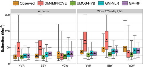
The distribution of the observations and forecasts, as illustrated by boxplots, during the testing period is shown in Figure 4. When considering all available observations when RH was less than or equal to 90%, the western sites (YVR and BBY), which had similar extinction distribution, were generally less variable and degraded than YCW, where the worst visibility conditions as portrayed by the 98th percentile was doubled of YVR at approximately 240 Mm⁻¹. The baseline model (GM-IMPROVE) generally overestimated extinction significantly at YVR and BBY, but only moderately underestimated at YCW. UMOS-HYB, the prototype based on UMOS postprocessed forecasts without any additional statistical training, had a good approximation of the median extinction but underestimated both the mean and the extremes at all stations. The difference in model performance between GM-IMPROVE and UMOS-HYB at YVR and BBY was largely attributable to the overestimation of PM_2.5 and NO₂ concentrations by GEM-MACH, as mentioned earlier. The other variations in model inputs and configuration, such as the PM speciation profile (GEM-MACH forecast vs. historical) and the algorithm used (revised IMPROVE vs. extended hybrid), did not contribute significantly to the poor model performance of GM-IMPROVE at the two sites. Both statistical prototypes, GM-MLR and GM-RF, were also in good agreement with the observations and had forecast higher peak extinction values, as characterized by the 75th and 98th percentile, than UMOS-HYB. The linear prototype, GM-MLR, predicted higher extreme events (98th percentile) than the nonlinear prototype, GM-RF, although both had underpredicted the extremes by approximately 5 to 40% depending on the station. Model performance for the worst 20% visibility conditions during daylight hours was also analyzed in detail, as these cases are of great concern in visual air quality forecasting and management. Approximately half of these cases occurred from April to September, which may be associated with stagnant meteorological conditions conducive to secondary aerosol formation. The median extinction values for the worst 20% visibility conditions were moderately underestimated by approximately 4 to 10% by the statistical prototypes (GM-MLR and GM-RF). This is expected, as the algorithms used in statistical model training generally minimized the model bias for the average extinction condition rather than the extremes. In addition, there may not have been a sufficient number of degraded visibility cases to properly train the prototypes in forecasting poor visual air quality conditions. Additional analyses such as resampling and boosted regression technique are recommended to potentially improve the model forecast during these infrequent but poor visual air quality episodes.

Figure 4. Boxplot of the observed and forecast extinction for all hours and during the worst 20% visibility conditions (daylight hours only), including all forecast lead times (1–48 hr) and model initiation hour (00:00 and 12:00 UTC), over the testing period (January–October 2012). The box indicates the interquartile range (25th to 75th percentile), the bar and solid circle indicates the median and average, respectively, and the whiskers indicate the 2nd to 98th percentiles.

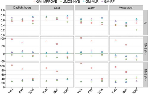
Figure 5 summarizes model performance statistics of the baseline model and developed prototypes averaged over all forecast lead times (1–48 hr) and model initiation hours (00:00 and 12:00 UTC) at the three sites. As corroborated by previous analyses, the baseline model, GM-IMPROVE, had skill in forecasting extinction during various daylight conditions with correlation coefficients (R) ranging from 0.37 to 0.70, although the normalized mean bias (NMB) and error (NME) were high at the western stations. The difference in baseline forecast performance between the stations may be attributable to GEM-MACH’s ability in forecasting both air quality and meteorological conditions in western versus eastern LFV. The statistical prototypes (GM-MLR and GM-RF) performed relatively well in comparison to GM-IMPROVE during daylight hours for both warm and cold season, where the R value ranged from 0.59 to 0.77 and the normalized mean error (NME) and bias (NMB) were generally 25 to 40% and less than 20%, respectively. UMOS-HYB also had modest improvements over the baseline model, with the exception of YCW where GM-IMPROVE performed well, during most daylight hours excluding poor visibility episodes. Additional analysis indicated that the poor UMOS-HYB forecast skill at YCW was due to a combination of errors in forecasting PM species contributions when using the historical monthly PM speciation profiles from Abbotsford to estimate extinction and an underestimation of RH (not shown). During poor visibility episodes as portrayed by the worst 20% category, both GM-MLR and GM-RF had noticeable improvements over GM-IMPROVE with R values ranging from 0.46 to 0.64. The NME and NMB of the statistical prototypes were approximately 20 to 30% and less than 20%, respectively. Substantial improvements over the baseline model in both NME and NMB were observed at YVR and BBY. Although the statistical prototypes performed similarly, GM-MLR performed the best at all three stations when considering all model forecast scores, especially during poor visibility episodes. These results also highlighted that UMOS-HYB, a prototype that did not require any additional statistical model training, can also provide reasonable forecasts during daylight hours for BBY and YVR, when using the more accurate statistical postprocessed UMOS-AQ PM_2.5 forecasts. In an operational setting, UMOS-HYB would likely be the most straightforward to implement and maintain as it utilizes outputs that are readily available and supported by the current RAQDPS infrastructure. Additional periodic model training and development of a data extraction and computation routine for persistence and antecedent air quality parameters would be required for the more precise and less biased GM-MLR prototype. It should also be mentioned that there would be instances when GM-MLR is unable to provide a forecast as the prototype requires the presence of all predictor variables that were used in model training. It is therefore recommended to implement the GM-MLR prototype with UMOS-HYB as a backup model to maximize both accuracy and availability.

Figure 5. Model performance statistics (correlation, normalized mean bias, and normalized mean error) of the different prototypes under various conditions during daylight hours averaged over all forecast lead times (1–48 hr) and two forecast initiation hours (00:00 and 12:00 UTC) at the three sites. The solid green line indicates the perfect skill score.

Visual air quality rating

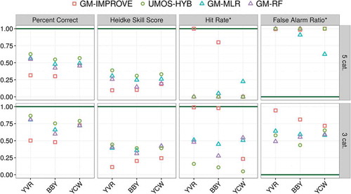
Figure 6 shows the categorical forecast skill scores for the baseline model and developed prototypes in predicting a full five-category and a condensed three-category VAQR index. The performance for a condensed three-category VAQR was investigated as the skill scores in forecasting the full index were only modest, where the best performing prototypes were approximately 55 to 60% correct depending on the station. Based on the percent correct and the Heidke Skill Score, GM-IMPROVE and UMOS-HYB performed the worst and best, respectively, at all stations. These findings are largely an artifact of the observed VAQR conditions in the LFV, where the majority of the daylight hours fall in the “excellent” and “good” categories. Models that tend to overestimate extinction, such as GM-IMRPOVE, would score lower than those that underestimate extinction. To get a better sense of the individual model performance, a contingency table illustrating the counts of VAQR forecasts and observations at YCW is shown in Table 2. Although the model performance of GM-IMPROVE at YCW is not representative of that at YVR and BBY, the other prototypes performed similarly at all stations. When the observed VAQR was “excellent,” the statistical prototypes tended to forecast “good,” and these were split between “fair” and “poor” when “poor” was observed. During “very poor” conditions, which occurred approximately 0.4% of the time during the testing period at YCW, the statistical prototypes were generally more optimistic and forecast for “poor.” When the VAQR is condensed into a three-category index, the best prototypes were found to be approximately 75 to 87% correct. Heidke Skill Score showed that the best prototypes had an approximate 35% and 40% improvement over that of random chance for the full and condensed VAQR, respectively. To assess their ability in forecasting poor visibility conditions, the hit rate and false alarm ratio for “very poor” and “poor and worse” categories, which occurred at less than 1% and 5%, respectively, were analyzed. While all four models had difficulties, GM-MLR and GM-RF performed marginally better with a hit rate and false alarm ratio of approximately 50% for the condensed index. For future work, it is recommended to develop statistical models, such as random forest or ordinal logistic regression, to be exclusively trained for forecasting VAQR instead of converting from extinction forecasts.

Table 2. Multicategory contingency table to verify VAQR forecasts at Chilliwack Airport (YCW) for models initialized at 00:00 and 12:00 UTC for forecast lead time 1–48 hr. Boldface values indicate the number of correct forecasts for each category.

		Excellent	Good	Fair	Poor	Very poor	Total (forecast)
GM-IMPROVE	Excellent	1377	1106	161	6	0	2650
	Good	597	1206	705	92	8	2608
	Fair	82	382	339	117	21	941
	Poor	3	66	109	49	11	238
	Very Poor	0	5	6	14	0	25
UMOS-HYB	Excellent	1349	773	89	2	0	2213
	Good	667	1765	675	81	20	3208
	Fair	36	216	544	179	20	995
	Poor	7	7	8	13	0	35
	Very Poor	0	4	4	3	0	11
GM-MLR	Excellent	639	225	19	1	0	884
	Good	1224	1516	236	5	0	2981
	Fair	189	968	905	144	7	2213
	Poor	7	56	160	113	24	360
	Very Poor	0	0	0	15	9	24
GM-RF	Excellent	220	34	2	0	0	256
	Good	1653	1700	242	3	0	3598
	Fair	181	987	874	134	8	2184
	Poor	5	44	202	141	32	424
	Very Poor	0	0	0	0	0	0
	Total (obs)	2059	2765	1320	278	40	6462

Figure 6. Visual Air Quality Rating (VAQR) forecast skill scores for the full (five-category) and condensed (three-category) index. VAQR forecasts are based on all available combination of forecast lead times (1–48 hr) and model initiation hours (00:00 and 12:00 UTC). Hit rate and false alarm ratio were examined for “very poor” and “poor and worse,” depending on the number of categories examined. The solid green line indicates the perfect skill score.

Case study—October 2012

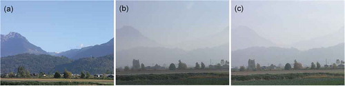
The October 2012 case study shows how visibility forecasts, in the form of hourly extinction and VAQR, can provide an added benefit to the public and air quality management agency during stagnant air quality episodes. Figure 7 illustrates the observed and forecasted air quality, visibility, and meteorological conditions during October 6–12, 2012, at Chilliwack Airport (YCW). Prior to October 9, the observed daytime PM_2.5 was generally low, less than 10 µg/m³, and was forecast well by both GEM-MACH and UMOS-AQ. On the evening of October 8, the observed PM_2.5 increased steadily to a peak concentration of 25 µg/m³, which later decreased but persisted at approximately 10 to 20 µg/m³ until midday on October 12. Air Quality Health Index (AQHI; Stieb et al. 2008) values of less than 4, corresponding to a low human health risk, were forecast for majority of the period. The health messaging associated with this event listed the air quality conditions as being ideal for outdoor activities for the general population (Stieb et al. 2008). While the ambient air quality conditions were considered good in terms of human health perspective, 1-hr optical reconstructed extinction values were high with VAQR of “poor” and “very poor.” These conditions were corroborated by the digital camera images taken at YCW as shown in Figures 8b and 8c, where the mountain ranges had nearly disappeared behind a white haze, in comparison to an example of “excellent” VAQR recorded earlier in the month (Figure 8a). Although both PM_2.5 and daytime RH were underestimated during this episode, poor visual air quality was forecast by both GM-MLR and GM-RF with 25 to 48 hr forecast lead times. Under similar atmospheric conditions, visibility forecasts can provide air quality reporting agencies with additional information to better tailor their public message and address concerns regarding visual impairment despite a lack of health concerns. The availability of reliable and timely visibility forecasts during periods of poor visual air quality can serve as a valuable outreach opportunity for local jurisdictions to promote both air quality and visibility management efforts by recommending practical ways to reduce emissions.

Figure 7. Time series of extinction (a), RH (b), PM_2.5 (c), and AQHI (d) from October 6 to 12, 2012, at Chilliwack Airport (YCW). Extinction forecasts were based on 25–48 hr forecast lead times at 00:00 UTC model initialization. The solid red line in panel (a) indicates the threshold above which visibility conditions are considered “poor” or worse based on the VAQR. The solid gray lines in panel (b) indicate the 75% and 90% RH threshold.

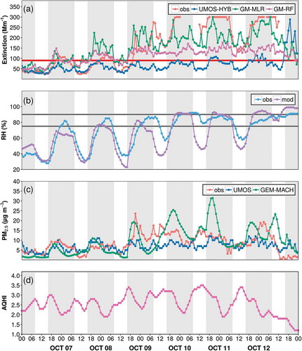
Figure 8. Digital camera imagery taken at Chilliwack Airport (NW direction) on October 3 at 04:00 p.m. PST (a), October 9 at 12:00 p.m. PST (b), and October 11 at 01:00 p.m. PST (c), when the VAQR was “excellent,” “very poor,” and “poor,” respectively.

Conclusion

This study has demonstrated the development and the potential use of air quality and meteorological forecasts from the Regional Air Quality Deterministic Prediction System (RAQDPS) to provide both numerical and categorical visibility forecasts with lead time up to 48 hr for three sites in the Lower Fraser Valley of British Columbia. A baseline model (GM-IMPROVE) was constructed using the revised IMPROVE algorithm based on unprocessed forecasts from the RAQDPS. Three additional prototypes (UMOS-HYB, GM-MLR, GM-RF) were also developed and assessed for forecast performance under various air quality and meteorological conditions.

A comparison of the forecasts with observational data (24-hr reconstructed extinction) indicated that although the baseline model, GM-IMPROVE, generally overestimated extinction over twofold at Burnaby South (BBY), it had skill in estimating the relative extinction contribution of the major PM species, including ammonium sulfates, ammonium nitrates, organic carbon, and elemental carbon. When visibility forecasts were compared with 1-hr optical reconstructed extinction, it was found that the three prototypes were in better agreement with the observed data in comparison to the GM-IMPROVE forecast at all stations. UMOS-HYB, a prototype based on postprocessed air quality forecasts without any additional statistical modeling, gave a good approximation of the observed median, but underestimated both the mean and the extremes. Model performance statistics indicated that both GM-MLR and GM-RF performed well in comparison to GM-IMPROVE during daylight hours for both warm and cold seasons at all stations. When considering all model forecast scores, especially during poor visibility episodes, GM-MLR was the best performing prototype at all three stations. In an operational setting, UMOS-HYB would be the most straightforward to implement, while additional periodic model training and development of a data extraction and computation routine would be required for the more accurate GM-MLR prototype. As GM-MLR requires the presence of all predictor variables used in model training, which may not always be available, it is recommended that GM-MLR prototype be implemented with UMOS-HYB as a backup to maximize both accuracy and availability.

In addition to numerical forecasts, the prototypes were assessed in their ability to forecast Visual Air Quality Rating (VAQR). Depending on the site of interest, the best performing prototypes were approximately 55 to 60% and 75 to 87% correct, when providing the full five-category and condensed-three category VAQRs, respectively. Model forecast skill scores such as percent correct and Heidke skill score were found to be reflective of the observed VAQR conditions in the LFV. Models that generally overestimated extinction had lower scores, as majority of the observed daylight hours fell in the “excellent” and “good” categories. GM-MLR and GM-RF tended to forecast “good” when the observed VAQR was “excellent” and were split between “fair” and “poor” when “poor” was observed. While all four models had difficulties in forecasting a “poor or worse” VAQR, GM-MLR and GM-RF performed marginally better with a hit rate and false alarm ratio of approximately 50%. For future work, it is recommended that statistical models based on random forest or ordinal logistic regression be developed to exclusively forecast the VAQR.

A case study, focusing on a period with poor visual air quality conditions yet low health risk, as estimated by the AQHI, illustrated that the developed statistical prototypes were able to forecast these episodes with lead time up to 48 hr. These forecasts, when supplemented with the existing air quality and health-based forecasts, can assist jurisdictions in formulating the appropriate air quality bulletins and recommendations. They can also provide a valuable outreach opportunity for local jurisdictions to promote air quality and visibility management efforts, when poor visual air quality episodes are forecasted. Although this paper focuses on the LFV, the developed modeling framework can be applied to all stations with air quality and meteorological forecasts across Canada, preferably those with PM speciation and visibility measurements if available. With the integration of near real-time wildfire emissions in the current operational air quality forecast system (FireWork; Pavlovic et al. 2016), there is a potential to provide valuable and timely visibility forecasts to assist jurisdictions in anticipating the visual air quality impacts during wildfire smoke events.

Additional information

Notes on contributors

Rita So

Rita So is an air quality scientist in the Air Quality Science Unit.

Andrew Teakles

Jonathan Baik is a systems developer in the Air Quality Science Unit.

Jonathan Baik

Roxanne Vingarzan is the Head of the Air Quality Science Unit.

Roxanne Vingarzan

Keith Jones is an atmospheric chemist in the Air Quality Science Unit, Prediction Services Directorate, Meteorological Services of Canada at Environment and Climate Change Canada, Vancouver, BC.

Keith Jones

Andrew Teakles is a research meteorologist in the Applied Environmental Prediction Science Atlantic, Prediction Services Directorate, Meteorological Services of Canada at Environment and Climate Change Canada, Halifax, NS.

References

- Anselmo, D., M. Moran, S. Ménard, V. Bouchet, P. Makar, W. Gong, A. Kallaur, P. A. Beaulieu, H. Landry, P. Huang, et al. 2010. A new Canadian air quality forecast model: GEM-MACH15. Paper presented at the 12th AMS Conference on Atmospheric Chemistry, Atlanta, GA, January 17–21.
- Antonopoulos, S., P. Bourgouin, J. Montpetit, and G. Croteau. 2011. Forecasting O3, PM25 and NO2 hourly spot concentrations using an updatable MOS methodology. In Air pollution modeling and its application XXI. NATO science for peace and security series C: Environmental security, ed. D. Steyn and S. Trini Castelli. Dordrecht, The Netherlands: Springer. 309–314.
- Arizona Department of Environmental Quality. 2003.Visibility index oversight committee final report: Recommendation for a phoenix area visibility index. http://www.phoenixvis.net/PDF/vis_031403final.pdf. (accessed April 17, 2018).
- Arnott, W. P., K. Hamasha, H. Moosmüller, P. J. Sheridan, and J. A. Ogren. 2005. Towards aerosol light-absorption measurements with a 7-wavelength aethalometer: Evaluation with a photoacoustic instrument and 3-wavelength nephelometer. Aerosol Sci. Technol. 39 (1):17–29. doi:10.1080/027868290901972.
- Breiman, L. 1996. Bagging predictors. Machine Learn. 24 (2):123–40. doi:10.1007/BF00058655.
- Breiman, L. 2001. Random forests. Berkeley, CA: Department of Statistics, University of California. https://www.stat.berkeley.edu/~breiman/randomforest2001.pdf ( accessed June 2, 2017).
- Breiman, L., and A. Cutler. 2004. Random forests. Berkeley, CA: Department of Statistics, University of California. https://www.stat.berkeley.edu/~breiman/RandomForests/cc_home.htm ( accessed June 2, 2017).
- British Columbia Visibility Coordinating Committee. 2015a.Working to clear the air in BC. http://www.clearairbc.ca/visibility/Documents/2013_15_BCVCC_annual_report.pdf. (accessed April 17, 2018).
- British Columbia Visibility Coordinating Committee. 2015b.The economic benefits of improving visual air quality in British Columbia’s Lower Fraser Valley. http://www.clearairbc.ca/visibility/Documents/EconomicBenefitsDiscussionPaper.pdf. (accessed April 17, 2018).
- British Columbia Visibility Coordinating Committee. 2017a. Working to clear the air in BC—British Columbia Visibility Coordinating Committee/Vancouver, BC 2015–2017 report.
- British Columbia Visibility Coordinating Committee. 2017b. Clear air BC. http://www.clearairbc.ca/Pages/default.aspx. (accessed June 2, 2017).
- Brewer, P., and T. Moore. 2009. Source contributions to visibility impairment in the southeastern and western United States. J. Air Waste Manage. Assoc. 59 (9):1070. doi:10.3155/1047-3289.59.9.1070.
- Carlson, K. 2009. Mountains that see, and that need to be seen: Aboriginal perspectives on degraded visibility associated with air pollution in the BC lower mainland and Fraser Valley. http://www.clearairbc.ca/visibility/Documents/Aboriginalperspectives.pdf. (accessed April 17, 2018).
- Chameides, W. L., H. Yu, S. C. Liu, M. Bergin, X. Zhou, L. Mearns, G. Wang, C. S. Kiang, R. D. Saylor, C. Luo, et al. 1999. Case study of the effects of atmospheric aerosols and regional haze on agriculture: An opportunity to enhance crop yields in China through emission controls? Proc. Natl. Acad. Sci. USA 96 (24):13626–33. doi:10.1073/pnas.96.24.13626.
- Chen, X., C. Lu, W. Liu, and Y. Zhang. 2013. A new algorithm for calculating the daytime visibility based on the color digital camera. Int. J. Computer Sci. Issues 10 (1):574–79.
- Dabek-Zlotorzynska, E., T. F. Dann, P. Kalyani Martinelango, V. Celo, J. R. Brook, D. Mathieu, L. Ding, and C. C. Austin. 2011. Canadian National Air Pollution Surveillance (NAPS) PM2.5 speciation program: Methodology and PM2.5 chemical composition for the years 2003–2008. Atmos. Environ. 45 (3):673–86. doi:10.1016/j.atmosenv.2010.10.024.
- Díaz-Uriarte, R., and S. Alvarez De Andrés. 2006. Gene selection and classification of microarray data using random forest. BMC Bioinformatics 7 (1):3. doi:10.1186/1471-2105-7-3.
- Dolan, S. 2016. Citizen science smart phone emission monitoring nextgen visibility measurement. Paper presented at Atmospheric Optics: Aerosols, Visibility, and the Radiative Balance, Jackson Hole, Wyoming, September 27–30.
- Ely, D. W., J. T. Leary, T. R. Stewart, and D. M. Ross. 1991. The establishment of the denver visibility standard. Paper presented at 84th Annual Meeting & Exhibition of the Air and Waste Management Association, Vancouver, British Columbia, June 16–21.
- Furberg, M., and K. Preston. 2005. Health and air quality 2005—PHASE II—Valuation of health impacts from air quality in the Lower Fraser Valley airshed. http://www.bc.lung.ca/pdf/health_and_air_quality_2005.pdf. (accessed April 17, 2018).
- Gallagher, J., and I. McKendry. 2011. Visibility perception in the Lower Fraser Valley, BC. www.clearairbc.ca/visibility/Documents/VisibilityPerceptionLFV2011.pdf. (accessed April 17, 2018).
- Gao, R. S., J. P. Schwarz, K. K. Kelly, D. W. Fahey, L. A. Watts, T. L. Thompson, J. R. Spackman, J. G. Slowik, E. S. Cross, J.-H. Han, et al. 2007. A novel method for estimating light-scattering properties of soot aerosols using a modified single-particle soot photometer. Aerosol Sci. Technol. 41 (2):125–35. doi:10.1080/02786820601118398.
- Grantz, D. A., J. H. B. Garner, and D. W. Johnson. 2003. Ecological effects of particulate matter. Environ. Int. 29 (2):213–39. doi:10.1016/S0160-4120(02)00181-2.
- Haider, W., J. Moore, D. Knowler, and D. Anderson. 2002. Estimating visibility aesthetics damages for AQVM. Ottawa, ON, Canada: Environmental Economics Branch, Environment Canada.
- Heidke, P. 1926. Berechnung des Erfolges und der Güte der Windstärkevorhersagen im Sturmwarnungsdienst. Geografiska Annal. 8:301–49.
- Jolliffe, I. T., and D. B. Stephenson. 2012. Forecast verification: A practitioner’s guide in atmospheric science, 2nd ed. Hoboken, NJ: John Wiley & Sons.
- Joint Working Group on Forecast Verification Research. 2009. Forecast verification—Issues, methods and FAQ. WWRP/WGNE Joint Working Group on Forecast Verification Research. http://www.cawcr.gov.au/projects/verification/verif_web_page.html#Introduction ( accessed May 25, 2017).
- Kellerhals, M. 2016. The Visual Air Quality (VAQR): A metric for visual air quality in the Lower Fraser Valley. Presented to the British Columbia Visibility Coordinating Committee, Vancouver, BC, June 24.
- Kluepfel, C. 2004. International verification workshop—Equitable skill score use in the U.S. National Weather Service. U.S. National Weather Program. http://www.cawcr.gov.au/projects/verification/Workshop2004/presentations/1.7_Kluepfel.pdf ( accessed May 25, 2017).
- Liaw, A., and M. Wiener. 2002. Classification and regression by randomForest. R News 2 (3):18–20.
- Liaw, A., and M. Wiener. Using Fortran original code by Leo Breiman and Adele Cutler, 2012. randomForest: Breiman and Cutler’s Random Forests for Classification and Regression. R package version 4.6.7.
- Lin, J., and J. Li. 2016. Spatio-temporal variability of aerosols over East China inferred by merged visibility-GEOS-chem aerosol optical depth. Atmos. Environ. 132:111–22. doi:10.1016/j.atmosenv.2016.02.037.
- Liu, M., M. Wang, J. Wang, and D. Li. 2013. Comparison of random forest, support vector machine and back propagation neural network for electronic tongue data classification: Application to the recognition of orange beverage and Chinese vinegar. Sensors Actuators B Chem. 177:970–80. doi:10.1016/j.snb.2012.11.071.
- Lowenthal, D., and N. Kumar. 2006. Light scattering from sea-salt aerosols at interagency monitoring of protected visual environments (IMPROVE) sites. J. Air Waste Manage. Assoc. 56 (5):636. doi:10.1080/10473289.2006.10464478.
- Lowenthal, D. H., and N. Kumar. 2003. PM2.5 mass and light extinction reconstruction in IMPROVE. J. Air Waste Manage. Assoc. 53 (9):1109. doi:10.1080/10473289.2003.10466264.
- Lumley, T., Using Fortran Code by Alan Miller. 2009. leaps: Regression subset selection. R package version 2.9. https://CRAN.R-project.org/package=leaps.
- Makar, P. A., W. Gong, C. Hogrefe, Y. Zhang, J. Zhang, G. Curci, R. Žabkar J. Milbrandt, U. Im, A. Balzarini, et al. 2014b. Feedbacks between air pollution and weather, part 2: Effects on chemistry. Atmos. Environ. 115:499–526. doi:10.1016/j.atmosenv.2014.10.021.
- Makar, P. A., W. Gong, J. Milbrandt, C. Hogrefe, Y. Zhang, G. Curci, R. Žabkar, U. Im, A. Balzarini, R. Baró, et al. 2015. Feedbacks between air pollution and weather, part 1: Effects on weather. Atmos. Environ. 115:442–69. doi:10.1016/j.atmosenv.2014.12.003.
- Malm, W. C., D. E. Day, S. M. Kreidenweis, J. L. Collett, and T. Lee. 2003. Humidity-dependent optical properties of fine particles during the big bend regional aerosol and visibility observational study. J. Geophys. Res. Atmos. 108 (D9):4279. doi:10.1029/2002JD002998.
- Malm, W. C., and J. L. Hand. 2007. An examination of the physical and optical properties of aerosols collected in the IMPROVE program. Atmos. Environ. 41 (16):3407–27. doi:10.1016/j.atmosenv.2006.12.012.
- Matsuki, K., V. Kuperman, and J. A. Van Dyke. 2016. The random forests statistical technique: An examination of its value for the study of reading. Sci. Stud. Reading 20 (1):20–33. doi:10.1080/10888438.2015.1107073.
- McNeill, R., and A. Roberge. 2000. The impact of visual air quality on tourism revenues in Greater Vancouver and the Lower Fraser Valley. http://www.clearairbc.ca/visibility/Documents/VisibiltyTourism-McNeill.pdf.
- Metro Vancouver. 2012. Station information: Lower Fraser Valley air quality monitoring network—December 2012. http://www.metrovancouver.org/services/air-quality/AirQualityPublications/LowerFraserValleyAirQualityMonitoringNetwork2012StationInformation.pdf.
- Metro Vancouver. 2015. 2014 Lower Fraser Valley air quality monitoring report. http://www.metrovancouver.org/services/air-quality/AirQualityPublications/2014_LFV_AQ_Monitoring_Report.pdf.
- Miller, A. 2002. Subset selection in regression. Boca Raton, FL: CRC Press.
- Mölders, N., and S. Gende. 2015. Impacts of cruise-ship entry quotas on visibility and air quality in glacier bay. J. Environ. Prot. 6 (11):1236–56. doi:10.4236/jep.2015.611109.
- Moosmüller, H., R. K. Chakrabarty, and W. P. Arnott. 2009. Aerosol light absorption and its measurement: A review. J. Quant. Spectrosc. Radiative Transfer 110 (11):844–78. doi:10.1016/j.jqsrt.2009.02.035.
- Moran, M., J. Chen, S. Ménard, R. Pavlovic, H. Landry, P.-A. Beaulieu, S. Gilbert, P.A. Makar, W. Gong, C. Stroud 2011. Two years of operational AQ forecasting with GEM-MACH15: A look back and a look ahead. Paper presented at the 10th annual CMAS Conference, Chapel Hill, NC, October 24–24. https://www.cmascenter.org/conference/2011/abstracts/moran_two_years_2011.pdf.
- Moran, M., S. Menard, D. Talbot, P. Huang, P. A. Makar, W. Gong, H. Landry, S. Gravel, S. Gong, L.-P. Crevier, et al. 2010. Particulate-matter forecasting with GEM-MACH15, a new Canadian air-quality forecast model. In Air pollution modelling and its application XX, ed. D. G. Steyn and S. T. Rao, 289–92. Dordrecht, The Netherlands: Springer.
- Moran, M., Q. Zheng, J. Zhang, R. Pavlovic, S. Ménard, and S. Mourad. 2012. Recent improvements to the representation of anthropogenic emissions in the canadian operational air quality forecast model (GEM-MACH). Paper presented at the 4th International Workshop on Air Quality Forecasting Research, Geneva, Switzerland, December 12–14.
- NOAA. 2017. Hazard mapping system fire and smoke product—Current HMS analysis. NOAA Office of Satellite and Product Operations. http://www.ospo.noaa.gov/Products/land/hms.html.
- Ogutu, J. O., H. Piepho, and T. Schulz-Streeck. 2011. A comparison of random forests, boosting and support vector machines for genomic selection. BMC Proceedings 5 (Suppl. 3):S11. doi:10.1186/1753-6561-5-S3-S11.
- Optec, Inc. 2006. Model NGN-2a Open air integrating nephelometer—Technical manual for theory of operation and operating procedures. Lowell, MA: Optec, Inc., October.
- Pavlovic, R., J. Chen, K. Anderson, M. D. Moran, P. A. Beaulieu, D. Davignon, and S. Cousineau. 2016. The FireWork air quality forecast system with near-real-time biomass burning emissions: Recent developments and evaluation of performance for the 2015 North American wildfire season. J. Air Waste Manage. Assoc. 66 (9):819–41. doi:10.1080/10962247.2016.1158214.
- Peng, H., A. R. Lima, A. Teakles, J. Jin, A. J. Cannon, and W. W. Hsieh. 2017. Evaluating hourly air quality forecasting in canada with nonlinear updatable machine learning methods. Air Qual. Atmos. Health 10 (2):195–211. doi:10.1007/s11869-016-0414-3.
- Pitchford, M. 2010.Assessment of the use of speciated PM2.5 Mass-calculated light extinction as a secondary PM NAAQS indicator of visibility. Memorandum to PM NAAQS Review Docket (EPA-HQ-OAR-2007-0492). http://www.epa.gov/ttn/naaqs/standards/pm/s_pm_2007_td.html.
- Pitchford, M., W. Maim, B. Schichtel, N. Kumar, D. Lowenthal, and J. Hand. 2007. Revised algorithm for estimating light extinction from IMPROVE particle speciation data. J. Air Waste Manage. Assoc.57 (11):1326. doi:10.3155/1047-3289.57.11.1326.
- Poduri, S., A. Nimkar, and S. Sukhatme. 2010. Visibility monitoring using mobile phones. http://robotics.usc.edu/~mobilesensing/visibility/MobileAirQualitySensing.pdf.
- Pryor, S. C., and R. J. Barthelmie. 2000. REVEAL II: Seasonality and spatial variability of particle and visibility conditions in the Fraser Valley. Sci. Total Environ.257 (2):95–110. doi:10.1016/S0048-9697(00)00490-3.
- Pryor, S. C., R. J. Barthelmie, R. M. Hoff, S. Sakiyama, R. Simpson, and D. Steyn. 1997. Reveal: Characterizing fine aerosols in the Fraser Valley, B.C. Atmosphere-Ocean 35 (2):209–27. doi:10.1080/07055900.1997.9649592.
- RWDI. 2006. Pacific Northwest air quality scenarios modelling project. Prepared for Environment Canada, Pacific & Yukon Region, Vancouver, BC, June 13.
- Snik, F., J. H. H. Rietjens, A. Apituley, H. Volten, B. Mijling, A. Di Noia, S. Heikamp, R. C. Heinsbroek, O. P. Hasekamp, J. M. Smit, et al. 2014. Mapping atmospheric aerosols with a citizen science network of smartphone spectropolarimeters. Geophys. Res. Lett. 41 (20):7351–58. doi:10.1002/2014GL061462.
- So, R., R. Vingarzan, K. Jones, and M. Pitchford. 2015. Modeling of time-resolved light extinction and its applications to visibility management in the Lower Fraser Valley of British Columbia, Canada. J. Air Waste Manage. Assoc. 65 (6):707–20. doi:10.1080/10962247.2015.1010750.
- So, R., R. Vingarzan, R. Kotchenruther, B. Taylor, R. Saari, and S. Hanna. 2014. Visibility. In The Georgia Basin–Puget Sound airshed characterization report, 165–86. Eds. Vingarzan R., So, R., and Kotchenruther R. Vancouver, BC, Canada.
- Stieb, D. M., R. T. Burnett, M. Smith-Doiron, O. Brion, H. H. Shin, and V. Economou. 2008. A new multipollutant, no-threshold air quality health index based on short-term associations observed in daily time-series analyses. J. Air Waste Manage. Assoc. 58 (3):435–50. doi:10.3155/1047-3289.58.3.435.
- Tang, I. N., A. C. Tridico, and K. H. Fung. 1997. Thermodynamic and optical properties of sea salt aerosols. J. Geophys. Res. 102 (D19):23269–75. doi:10.1029/97JD01806.
- Teakles, A., J. Baik, J. Montpetit, S. Antonopoulos, C. Saad, and N. Saran. 2017a. PROGNOS: A new MSC initiative to renew the operational statistical post-processing infrastructure. Paper presented at the 8th International Workshop on Air Quality Forecasting Research, Toronto, Canada, January 10–12.
- Teakles, A. D., R. So, B. Ainslie, R. Nissen, C. Schiller, R. Vingarzan, I. McKendry, A. M. Macdonald, D. A. Jaffe, A. K. Bertram, et al. 2017b. Impacts of the July 2012 Siberian fire plume on air quality in the Pacific Northwest. Atmos. Chem. Phys. 17 (4):2593–611. doi:10.5194/acp-17-2593-2017.
- U.S. Environmental Protection Agency. 1999. Regional haze regulations—Final rule. Fed. Reg. 64 (126). https://www.gpo.gov/fdsys/pkg/FR-1999-07-01/pdf/99-13941.pdf.
- Wan, J., M. Lin, C. Chan, Z. Zhang, G. Engling, X. Wang, I. Chan, and S. Li. 2011. Change of air quality and its impact on atmospheric visibility in central-western Pearl River Delta. Environ. Monit. nd Assess. 172 (1):339–51. doi:10.1007/s10661-010-1338-2.
- Wilson, L. J., and M. Vailée. 2002. The Canadian Updateable Model Output Statistics (UMOS) system: Design and development tests. Weather Forecast. 17. doi:10.1175/1520-0434(2002)017<0206:TCUMOS>2.0.CO;2.
- Zhang, H., and T. Casey. 2000. Verification of categorical probability forecasts. Weather Forecast. 15 (1):80–89. doi:10.1175/1520-0434(2000)015<0080:VOCPF>2.0.CO;2.
- Ziegler, A., and I. R. König. 2014. Mining data with random forests: Current options for real‐world applications. Wiley Interdiscip. Rev. Data Mining Knowledge Discovery 4 (1):55–63.