Visibility impacts at Class I areas near the Bakken oil and gas development

ABSTRACT

Oil and gas activities have occurred in the Bakken region of North Dakota and nearby states and provinces since the 1950s but began increasing rapidly around 2008 due to new extraction methods. Three receptor-based techniques were used to examine the potential impacts of oil and gas extraction activities on airborne particulate concentrations in Class I areas in and around the Bakken. This work was based on long-term measurements from the Interagency Monitoring of Protected Visual Environments (IMPROVE) monitoring network. Spatial and temporal patterns in measured concentrations were examined before and after 2008 to better characterize the influence of these activities. A multisite back-trajectory analysis and a receptor-based source apportionment model were used to estimate impacts. Findings suggest that recent Bakken oil and gas activities have led to an increase in regional fine (PM_2.5—particles with aerodynamic diameters <2.5 µm) soil and elemental carbon (EC) concentrations, as well as coarse mass (CM = PM₁₀–PM_2.5). Influences on sulfate and nitrate concentrations were harder to discern due to the concurrent decline in regional emissions of precursors to these species from coal-fired electric generating stations. Impacts were largest at sites in North Dakota and Montana that are closest to the most recent drilling activity.

Implications: The increase in oil and gas activities in the Bakken region of North Dakota and surrounding areas has had a discernible impact on airborne particulate concentrations that impact visibility at protected sites in the region. However, the impact has been at least partially offset by a concurrent reduction in emissions from coal-fired electric generating stations. Continuing the recent reductions in flaring would likely be beneficial for the regional visual air quality.

Introduction

Modern techniques of oil and gas extraction, including horizontal drilling and hydraulic fracturing (fracking), have facilitated cost-effective recovery of previously untapped oil and gas reserves in the Bakken region of western North Dakota, eastern Montana, southeastern Saskatchewan, and southwestern Manitoba (Figure 1). Production of oil in North Dakota increased from a few million barrels per month in 2000 to over 35 million barrels in 2015 (Allen 2016; North Dakota Industrial Commission, Department of Mineral Resources, Oil and Gas Division 2016; Prenni et al. 2016). More recently, there was a decline in the number of new wells drilled as the oil industry reacted to price reductions beginning in late 2014, with oil production leveling off and then beginning to decline in 2015. For example, the number of active wells in their initial phase in North Dakota on the same day (April 22) each year during 2012–2016 show 210 active wells in 2012, 186 and 187 in 2013 and 2014, respectively, 88 in 2015, and 29 in 2016 (North Dakota Industrial Commission 2016). Known air emissions from drilling, hydraulic fracturing, pumping, extraction, flaring, construction, transportation, and secondary population growth associated with oil and gas activities include carbon dioxide, carbon monoxide, elemental carbon (EC), benzene, polycyclic aromatic hydrocarbons, and other volatile organic compounds (VOCs), methane, hydrogen sulfide, nitrogen oxides (NO_x), dust, and sulfur dioxide (SO₂) (Allen 2016; Johnson et al. 2017a, 2017b; Prenni et al. 2016). These emissions may contribute to visibility impairment directly from primary emissions of EC, fine (PM_2.5—particles with aerodynamic diameters <2.5 µm) dust and coarse mass (CM = PM₁₀–PM_2.5) and indirectly through the production of secondary particulate matter from gaseous air pollutants, including NO_x, SO₂, and VOCs. For example, Evanoski-Cole et al. (2017) have shown that nitrate derived from oil and gas emissions was a major contributor to haze episodes in the region during the Bakken Air Quality Study, and Prenni et al. (2016) showed that oil and gas activities were the primary drivers for trends in black carbon during that same study.

Figure 1. Study area map. Stars are IMPROVE sites used in the analyses. See Table 2 for site names and other details. Active oil and gas wells are shown as small dots, and electric generating units are indicated by circled Xs. Data are valid as of 2014.

A recent modeling study has shown that oil and gas activities are having a negative impact on air quality in some Class I areas in the western United States (Thompson et al. 2017). Class I areas are large national and international parks and wilderness areas that are given the strongest air quality protection, including for visibility. There are three Class I areas in the Bakken region: Lostwood National Wildlife Refuge (LOST), Medicine Lake National Wildlife Refuge (MELA), and Theodore Roosevelt National Park (THRO). In accordance with the Clean Air Act, the U.S. Environmental Protection Agency (EPA) issued the 1999 Regional Haze Rule (EPA 1999, 2003; Murphy et al. 2011; Hand et al. 2014), requiring states to work with federal agencies to develop and implement plans to reduce the air pollution that causes visibility impairment and to make reasonable progress toward reaching natural conditions within 60 yr. These and other air quality regulations have had a positive effect, helping to decrease airborne particulate matter across the country an average of 35% since 2000 (Murphy et al., 2011; Hand et al., 2014; EPA 2016a, 2016b; Malm et al. 2017). However, data from the Interagency Monitoring of Protected Visual Environments (IMPROVE) network showed that the Bakken area has had anomalous upward trends in some fine particulate species during winter months (Hand et al. 2012) and experienced a smaller decrease in aerosol light extinction than in the rest of the United States, where scattering has decreased substantially (Hand et al. 2014).

The motivation behind this work is to better understand impacts to visibility in nearby Class I areas due to emissions from oil and gas extraction in the Bakken region. Specifically, we examine the association between speciated airborne fine particle concentrations and associated light extinction in the region and the multiyear increase in oil and gas extraction to determine which types of particles are driving the trends in visibility. Air mass back trajectories are also used to investigate the potential impacts of emissions from the Bakken region on rural and remote areas nearby and in surrounding states. Finally, a back-trajectory-based receptor model is used to estimate the fraction of several species of fine particulates arriving at Class I areas in and near the Bakken region from various source regions.

Emission trends

In a typical oil and gas well, approximately two-thirds to three-fourths of the direct air emissions occur during the initial drilling, fracturing, and flow-back activities within the first few days to few weeks (Allen 2016). Later, during the production phase, the well itself emits much less, although emissions from trucking, flaring, leaks, surface disturbance, and secondary population growth continue. Flaring has been a particular problem in the Bakken, where in 2013 approximately one-third of all gas was flared due to the lack of infrastructure to collect and transport the gas. Although flaring reduces emissions of hazardous air pollutants and greenhouse gases, it can be a significant source of other pollutants such as black carbon (Schwarz et al. 2015; Weyant et al. 2016). In 2014, the North Dakota Industrial Commission set goals to reduce the percentage of flared natural gas, and flaring has since decreased dramatically (U.S. Energy Information Administration 2016), falling to 10% in March 2016.

Besides oil and gas activities, other potential sources of fine particulate matter (PM_2.5) and precursors in the region include power plants, oil sands and related activity in Canada, agriculture, refineries, a coal gasification plant, and fires. Emission trends for North Dakota are shown in Figure 2. Statewide air pollutant emissions are estimated by the EPA National Emissions Inventory (NEI) based on data submitted by the states (EPA 2016a, 2016b). NEI emissions are estimated in detail every 3 yr, including 2002, 2005, 2008, 2011, and 2014. Some large point sources, such as electric generating units (EGUs), are equipped with continuous emission monitors that provide more accurate and frequent data. Emissions from nonmonitored sources are modeled, and the model formulations and inputs can change from one estimation period to the next. In addition, for these sources, data for non-NEI years are linearly interpolated between the NEI estimates. Consequently, the emissions are subject to large and varying uncertainties and biases, so the trends are considered approximate.

Figure 2. Annual emissions of (a) NO_x, (b) SO₂, (c) VOCs, and (d) PM_2.5 in North Dakota, 2002–2015, from petroleum and related industries and other categories that were large contributors. Data for SO₂ are from North Dakota (Hyatt 2017), all other data are from EPA (EPA 2016a).

Figure 2 shows estimated annual mean emissions of NO_x, SO₂, VOCs, and PM_2.5 in North Dakota during 2002–2015 for petroleum and related industries and other categories of large emitters for each species. Trends in PM₁₀ and ammonia are not shown, since the PM₁₀ trend is very similar to PM_2.5 and ammonia emissions had temporal step functions that did not appear realistic. Data for SO₂ are from the state of North Dakota because the 2011 and 2014 NEI data were generated using different input data, resulting in erroneous emission estimates (Hyatt 2017, Personal communication). Reanalyzed sulfur dioxide emissions for North Dakota. Received November 22, 2017). All other data are from EPA (EPA 2016a). Emissions from petroleum and related industries were very low for all air pollutants until about 2008–2010, when emissions began to climb, especially for VOCs, and secondarily for NO_x.

SO₂ emissions from petroleum and related industries were low compared with other sources in the state, due to the low sulfur content of the fuels in the Williston Basin.

NO_x emissions from electric utilities were historically much greater than from petroleum and related industries, but emissions from EGUs have been declining such that NO_x emissions from the two categories are now nearly equal.

Statewide PM_2.5 emissions have steadily increased, although the apparent increase between 2011 and 2014 was due to a methodological change in which the influence of precipitation on dust production was not considered in 2014 as it had been in previous NEI years (EPA 2016a, 2016b). EPA does not attribute PM_2.5 and PM₁₀ directly to oil and gas activities, putting the majority of the total in the miscellaneous category, which includes unpaved road dust, agricultural crops, livestock dust, and waste disposal (EPA 2016b). However, some of the increase could be related to trucking and secondary population growth associated with oil and gas. Nationally, the largest sources for primary emissions of PM_2.5 and PM₁₀ are road dust from unpaved and paved roads, construction, agriculture, and fires, including wild fires, prescribed fires, and residential wood combustion (EPA 2016b). Increased truck traffic due to oil and gas extraction can be significant, as approximately 2000 truckloads of materials are needed during the first year of a new well in the Bakken (North Dakota Department of Mineral Resources 2013). This truck traffic can generate pollutants typical of diesel engines, as well as a significant amount of fugitive dust (Bar-Ilan et al. 2011). EPA also lists mobile nonroad equipment as a major source of black carbon. (EPA 2016b).

Table 1 shows the multiyear means of statewide emissions for these and other air pollutants in North Dakota averaged over the earlier years, 2002–2007, when there was relatively little oil and gas activities in the region, and later years, 2008–2015, when oil and gas production was increasing rapidly. These values should be considered approximate due to the methodological changes as discussed above. Despite the rapid growth of oil and gas activities, SO₂ emissions were slightly lower in the later years than the earlier years and NO_x emissions were essentially unchanged. Conversely, VOC, PM_2.5, and PM₁₀ emissions were all greater in the later years. The largest increase, more than a factor of 5, was for VOCs. There was a 50% increase in PM_2.5 emissions and a 26% increase in PM₁₀, although these increases were overestimated due to the NEI calculation differences in 2014. Emission data are not used as input in the back-trajectory models discussed in the following sections but can help interpret the results.

Table 1. Approximate mean emission estimates for North Dakota during the early years, 2002–2007, and later years, 2008–2015, and the percent change between the two time periods.

Pollutant	Mean ND emissions (1000 tons/yr) Early years/Later years	Change
SO2	157/105	−33%
NOx	174/173	−0%
VOCs	46/316	+580%
PM2.5	70/106	+50%
PM10	387/488	+26%

Note. Data for SO₂ are from the state of North Dakota. All other values are from EPA. See text for discussion of caveats in emission trends.

Particulate matter concentrations and light extinction

Reconstructed light extinction

To understand the relative importance of PM_2.5 and its major constituents, including sulfate, nitrate, soil, organic carbon (OC), and EC, as well as CM to visibility in the region, trends in these concentrations from the IMPROVE monitoring network (Malm et al. 1994, 2017; Hand et al. 2012, 2014) were examined. IMPROVE collects integrated, 24-hr filter samples every 3 days. Data from 14 sites were used to calculate multiyear trends and in two receptor-based analyses. For some analyses, these sites were grouped into three categories: Group 1 for the sites closest to the Bakken, Group 2 for sites to the southwest, and Group 3 for sites to the east (Figure 1). Because the predominant wind direction in the midlatitudes is generally westerly, Group 3 sites should be downwind of the Bakken region more often than Group 2 sites. It should be noted that sites in Groups 2 and 3 can be several hundred kilometers from the Bakken region and so are also influenced by other sources nearer to these sites. For example, the coal-fired EGUs in Minnesota as shown in Figure 1 likely have a larger influence on Great River Bluffs (GRRI) than do Bakken oil and gas emissions. Site details and locations are shown in Table 2 and Figure 1. IMPROVE concentrations for 2002–2015 were used in the analyses. The time periods were classified as “early years” for 2002–2007 and “later years” for 2008–2015. The early years are prior to the rapid increase in oil and gas activities in the Bakken region (Prenni et al. 2016).

Table 2. Site information for the 14 IMPROVE sites used in the back-trajectory analysis.

Site name	Code	U.S. state	Group	Latitude (°N)	Longitude (°W)	Elevation (m AMSL)
Lostwood NWR	LOST	ND	1 (Close)	48.642	102.402	696
Theodore Roosevelt NP South Unit	THRO	ND		46.895	103.378	852
Medicine Lake NWR	MELA	MT		48.487	104.476	606
Fort Peck IR	FOPE	MT		48.500	105.300	638
UL Bend NWR	ULBE	MT	2 (Southwest)	47.582	108.720	891
Northern Cheyenne IR	NOCH	MT		45.500	106.600	1283
Thunder Basin NG	THBA	WY		44.600	105.300	1195
Cloud Peak WA	CLPE	WY		44.300	107.300	2470
Wind Cave NP	WICA	SD		43.558	103.484	1296
Badlands NP	BADL	SD		43.744	101.941	736
Blue Mounds SP	BLMO	MN	3 (East)	43.500	96.200	473
Great River Bluffs SP	GRRI	MN		43.800	91.400	370
Voyageurs NP	VOYA	MN		48.583	93.167	429
Boundary Waters CA	BOWA	MN		47.946	91.496	526

Note. AMSL = above mean sea level; CA = Canoe Area; IR = Indian Reservation; NG = National Grassland; NP = National Park; NWR = National Wildlife Refuge; SP = State Park; WA = Wilderness Area.

The particulate species that contribute to long-term average regional visibility conditions in the north-central United States were linearly combined to calculate reconstructed aerosol light extinction by the revised IMPROVE equation (IMPROVE 2016; Pitchford et al. 2007). Multiyear, multisite averages of these reconstructions are summarized in Table 3. Finer temporal and spatial scale exploration of the data, including daily extinction budgets, is available interactively on the Federal Land Manager Environmental Database (NPS 2017) and the IMPROVE Web site (IMPROVE 2016). The goal of the 1999 Regional Haze Rule (EPA 1999) is to protect visibility on the least-impaired days, while improving conditions on the most-impaired days, so conditions on both ends of the spectrum, as well as the mean, are of interest. Table 3 shows values for the “Worst” days corresponding to the average of the 20% highest extinction values for that time period, the “Best” days corresponding to the average of the 20% lowest extinction values, and the mean for “All” observations. The percentages in the table are the means of the extinction due to the individual species divided by the mean of the total aerosol extinction, or the ratio of the means, as opposed to the mean of the ratios, which would generate somewhat different values. The ratio of the means method gives days with higher concentrations a larger influence on the ratios. For all three levels, visibility decreases (or light extinction increases) going from west to east, with Group 2 having the lowest light extinction and Group 3 having the highest. In nearly all cases, on a multiyear, multisite average basis, light extinction was lower in the later years, 2008–2015, as compared with sites in the same regional group in the earlier years, 2002–2007. This is true for all three site groups and also for the best and worst extinction ends of the visibility spectrum, except for the worst level for Group 1, where the later years had slightly higher extinction. This is consistent with national trends (Hand et al. 2014). The declining aerosol extinction values are likely mostly due to decreasing emissions from EGUs over this same time period as shown in Figure 2.

Table 3. Multiyear and multisite averages of aerosol light extinction for IMPROVE sites (IMPROVE 2016).

Group	Bext level	Total aerosol extinction (1/Mm)	% Ammonium sulfate	% Ammonium nitrate	% Organic matter	% Elemental carbon	% Fine soil	% Coarse mass	% Sea salt
1	Worst	53.7/54.3	36/32	31/27	20/25	5/5	1/2	7/9	0/1
Close		(4/6)	(5/5)	(6/5)	(6/10)	(1/1)	(0/0)	(2/2)	(0/1)
	All	26.1/25.4	37/35	23/22	19/21	5/5	2/2	12/13	0/1
		(4/4)	(8/7)	(8/7)	(8/11)	(1/1)	(0/1)	(3/3)	(0/1)
	Best	9.6/8.6	38/38	13/13	18/18	7/6	3/3	19/20	1/1
		(0.5/0.5)	(4/4)	(2/2)	(2/2)	(1/1)	(0/0)	(3/2)	(0/0)
2	Worst	38.4/35.9	31/26	13/11	36/43	7/6	2/3	11/11	0/1
SW		(3/5)	(4/4)	(3/3)	(8/16)	(1/2)	(0/0)	(2/2)	(0/1)
	All	17.6/15.7	36/33	12/11	29/32	7/6	3/4	13/17	0/1
		(2/3)	(6/7)	(4/3)	(11/27)	(2/4)	(1/1)	(3/3)	(0/1)
	Best	5.5/4.6	38/39	11/11	21/21	9/6	4/4	17/17	0/1
		(0.2/0.2)	(3/3)	(1/1)	(2/2)	(1/2)	(0/0)	(2/2)	(0/0)
3	Worst	106.7/82.2	41/30	39/44	12/16	4/4	1/1	4/5	0/1
East		(10/9)	(8/5)	(9/9)	(3/8)	(1/1)	(0/0)	(1/1)	(0/0)
	All	45.9/36.0	41/34	32/33	14/17	5/5	1/1	7/8	1/2
		(8/6)	(13/8)	(13/12)	(5/10)	(1/1)	(0/0)	(2/2)	(0/1)
	Best	14.2/10.9	42/39	18/17	17/19	7/7	1/2	13/15	1/2
		(0.7/0.6)	(4/4)	(3/3)	(2/2)	(1/1)	(0/0)	(2/2)	(1/1)

Note. There are approximately 100 observations per site per year. Values are early years/later years. The standard deviations are shown in parentheses below the means. Early years are 2002–2007; later years are 2008–2015. “Worst” extinction level is the average of the highest 20% of reconstructed aerosol extinction; “Best” is the average of the lowest 20%, and “All” is the average of all observations with a complete set of aerosol measurements. Percent was calculated by dividing the mean scattering due to the species by the mean of the total aerosol light extinction. Site groupings are shown in Figure 1 and Table 2. No. 1/Mm stands for inverse megameter not inverse molar meter.

Trends in particulate matter concentrations

Concentration trends for the individual particulate species are discussed below in order from those with the greatest impact on extinction to those with the least. Figure 3 shows the Theil-Sen slopes (Theil 1950) for the changes in concentrations for all sites and species during 2002–2015. The Theil-Sen analysis is a nonparametric technique specifically designed to reduce the influence of outliers to generate an overall average trend for the time period of interest. Its greatest power to detect trends is when there is monotonic change, but it maintains skill even when the trend has a different functional shape such as a step change (Hess, Iyer, and Malm 2001). The level of significance at each site is also shown in Figure 3 and was assessed for P values of 0.1, 0.5, 0.01, and 0.001. Trends that were not significant at the P = 0.1 level were termed insignificant.

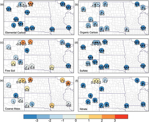
Figure 3. Theil-Sen slopes for 2002–2015 in percent per year for 14 IMPROVE sites in the Bakken region for (a) EC, (b) OC, (c) fine soil, (d) sulfate, (e) CM, and (f) nitrate concentrations. Symbols inside the circles indicate the significance of the slope based on P values. ***P < 0.001; **P < 0.01; *P < 0.05; ⁺P < 0.1; ^-P > 0.1.

Sulfate

The largest average contributor to aerosol extinction at all 14 sites was sulfate, contributing 36–41% on average in the early years, dropping to 33–35% in the later years. The fraction of aerosol extinction due to sulfate on the worst days also declined, from 31–41% in early years to 26–32% in later years. The contribution from sulfate on the best days remained relatively stable at 38–42% in the early years and 38–39% in the later years.

The highest mean concentrations of sulfate were at the southeasternmost sites, in southern Minnesota, and lowest at the sites farthest west. However, for the four close-in, Group 1 sites, Lostwood had the highest mean concentration, and it was more than 20% higher than the next highest value at Medicine Lake. There is a general trend of decreasing concentrations with time, consistent with the trends of decreasing EGU emissions. On an annual basis, all sites have statistically significant negative slopes for sulfate. The largest decrease, 8%/yr, was at Great River Bluffs in southeastern Minnesota. However, sulfate concentrations at the eastern Montana sites, Fort Peck (FOPE) and Medicine Lake, as well as Cloud Peak (CLPE) in northeastern Wyoming, have decreased more slowly than at other sites, at less than 3%/yr. The smaller decreases at these sites close to the Bakken region indicate a potential influence on sulfate concentrations from oil and gas activities, although any increase in SO₂ emissions from these sources was likely offset by the larger downward trend due to reductions in EGU emissions.

Nitrate

The second largest mean contributor to aerosol extinction was either nitrate or OC, depending on region. Nitrate contributed a larger fraction in Groups 1 and 3, whereas OC and CM were larger fractions on average in Group 2. The fraction of aerosol extinction due to nitrate changed very little from the early years to the later years. This was true for all three regional groups and for best and worst days as well as on average. The mean fraction due to nitrate was 12–32% in early years and 11–33% in later years. The biggest change was for the worst days in Group 3, where the nitrate contribution increased from 39% to 44%. In contrast, the nitrate fraction declined from 31% to 27% for worst days in Group 1. The fraction due to nitrate was highest in Group 3 and lowest in Group 2, with the Bakken area sites in Group 1 falling in the middle. Ammonium nitrate forms where combustion sources produce nitrogen oxides, which oxidize in the atmosphere and react with ammonia (Seinfeld and Pandis 1998). There was more agricultural activity and so likely more ammonia emissions near Group 3 than in the two regions farther west. In the Bakken region, it has been shown that stagnation events can lead to high concentrations of ammonium nitrate in winter (Evanoski-Cole et al. 2017).

Like sulfate, the highest mean nitrate concentrations were at the two southern Minnesota sites. The northern sites in Groups 1 and 2, Lostwood, Fort Peck, and Medicine Lake, had the highest mean values. The annual mean at Lostwood was a factor of 7 higher than at Cloud Peak (CLPE). Nitrate increased, although insignificantly, by 0.2%/yr at Fort Peck and Medicine Lake. All other sites decreased by 1–5%/yr. The largest monthly increases in nitrate were during May and June at Fort Peck, Medicine Lake, Theodore Roosevelt, and Lostwood, with the highest statistically significant increase being 10%/yr at Fort Peck in both months.

Organic matter

Organic matter (OM), estimated by OC × 1.8 (Pitchford et al. 2007; IMPROVE 2016), was the second highest contributor to aerosol extinction and was greater than nitrate at the southwestern sites in Group 2 and was the third largest fraction in Groups 1 and 3. The average OM fraction increased a few percentage points from 14–29% in the early years to 17–32% in the later years. On the worst visibility days in the southwestern group, OM had a larger impact than sulfate, probably due to wildfire events on those days. Controlled burns, residential wood combustion, and anthropogenic and biogenic secondary organic aerosol from VOCs also contribute to OM (EPA 2016b; Schichtel et al. 2017). OM was more spatially uniform than sulfate and nitrate, with the highest concentrations again in southern Minnesota. There was a western local maximum at Northern Cheyenne (NOCH), and the lowest mean was at Cloud Peak. All sites showed declines in annual average concentrations, although most sites had small, insignificant increases during the summer.

Coarse mass

CM contributed 7–13% to aerosol extinction on average in the early years and 8–17% in the later years. The mean fraction of aerosol extinction due to CM was about twice as high in Groups 1 and 2 as in Group 3. For Group 2, CM was a slightly larger fraction of the average aerosol extinction than nitrate. It had a lower fractional contribution on the worst visibility days and was a larger fraction on the best days in all groups. A typical source of CM is wind-blown dust from disturbed soil, which could be due to oil and gas extraction, mining, transportation, construction, or agriculture. (EPA 2016b) The maximum mean CM concentration was at Blue Mounds (BLMO) in southeastern Minnesota, and concentrations declined to the west, east, and north. Most sites east and north of a diagonal line from Blue Mounds, northwest to Fort Peck, increased 0–3%/yr, whereas those southwest of this line declined insignificantly at <1%/yr.

Elemental carbon

On average, EC contributed 5–7% in the early years and 5–6% in the later years, with a slightly higher fractional contribution on the best days than the worst days in all groups. On an annual average basis, concentrations at Lostwood increased significantly at about 3%/yr, whereas concentrations at all remaining sites declined by 3–6%/yr and many with significance at the P = 0.005 level. Typical large sources of EC in the United States are fires and emissions from diesel equipment (EPA 2016b; Schichtel et al. 2017). Flares may also contribute.

Fine soil

Fine soil was 1–3% of reconstructed aerosol light extinction in the early years and 1–4% in later years. Like EC, it had larger fractional contributions to extinction on the best days. There were insignificant, although increasing, concentrations of fine soil at three sites. Two of them, Lostwood and Medicine Lake, are in the Bakken area. Blue Mounds is in southwestern Minnesota. All other sites had flat or decreasing values. The spatial pattern was different from previously discussed species, with the greatest mean concentration at Thunder Basin, Wyoming (THBA), near coal mining activity.

Sea salt

As expected, for these mid-continental sites, sea salt contributed very little, 0–2%.

Back-trajectory residence times

Air mass transport patterns were examined with hourly ensemble back trajectories started at 10 m above ground, with a maximum length of 5 days, for 14 IMPROVE sites for 2002–2015 using version 4.9 of the Hybrid Single-Particle Lagrangian Integrated Trajectory (HYSPLIT) model (Draxler and Hess 1998; Stein et al. 2015). In ensemble mode, HYSPLIT generates 27 trajectories for each start time by using start points at the specified location, as well as 0.01 sigma units above and below and eight surrounding grid cells. Ensemble mode helps mitigate the sensitivity of HYSPLIT to wind shear, especially when it occurs near the start point, and is an inexpensive method to account for dispersion (Gebhart, Schichtel, and Barna 2005; Schichtel and Husar 1997). Gridded input meteorological data for the long-term analyses are from the North American Regional Reanalysis (NARR) with a horizontal grid resolution of 32 km (Mesinger et al. 2006). There are NARR data in HYSPLIT-ready format for 1979 to present, making it ideal for long-term trend analyses. A finer-scale data set, the North American Mesoscale Model on a 12-km grid (NAM12) (Janjic 2003), is available for 2008 and later, so these data were also used for later years.

Back-trajectory residence time analyses are a long-established method to examine air mass transport pathways (AshbaughMalm, & Sadeh 1985; Poirot and Wishinsky 1986). An end point, defined as the position of the air mass at a given time, is calculated hourly for each trajectory. A residence time matrix consists of the fraction of total end points in each 0.1° grid cell. Residence time analysis shows the upwind areas that can potentially contribute airborne concentrations to a receptor during average conditions or for specific time periods that are of interest for various reasons, such as seasonality, high or low concentrations, or meteorological conditions. Each individual trajectory has uncertainty that increases as the trajectory length increases (Stohl 1998), but if the errors are random rather than systematic, overall error in the average pathway is reduced by aggregating many trajectories (Gebhart, Schichtel, and Barna 2005).

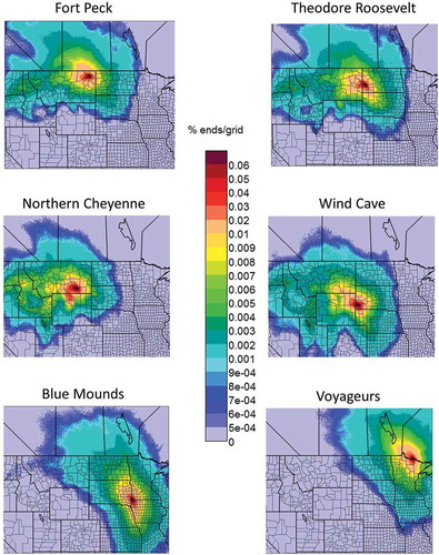
The predominant transport pathways for air masses arriving at two locations from each regional group for 3-day back trajectories during 2002–2015 are shown in Figure 4. Within each group, the transport patterns tended to be similar, although offset by start location, whereas the differences between the regional groups were larger. Group 1 sites, illustrated by Fort Peck and Theodore Roosevelt, had winds mostly from the west and northwest. Transport to Group 2 sites shown for Northern Cheyenne and Wind Cave was more westerly, and there was evidence of channeling through major terrain features of the western United States, such as the Snake River valley in southern Idaho. For sites to the east, illustrated by Blue Mounds and Voyageurs, air masses arrive most commonly from the northwest or southeast. Emissions from the Bakken region can reach all sites in 3 days or less, with Group 1 sites being impacted most often.

Figure 4. Back-trajectory overall residence times showing where air masses resided during the 3 days prior to arriving at each of six sites during 2002–2015. Top row is two sites in Group 1 (closest to Bakken), middle row is sites in Group 2 (southwest), and bottom row is sites in Group 3 (east).

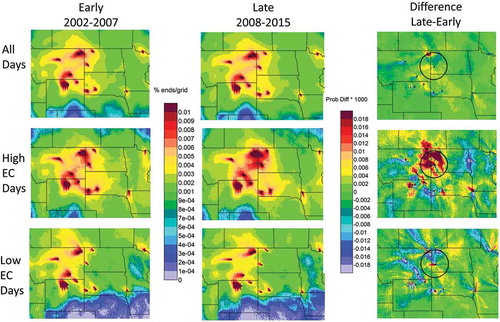
For the following analyses, high concentrations were defined as those at the 90th percentile or greater at each site during the analysis period, either 2002–2007 or 2008–2015; similarly, low concentrations were those at the 10th percentile or lower. For example, Figure 5 shows the results of summing the residence time matrices for all 14 sites, for all days, for days with high EC concentrations, and for days with low EC concentrations. The left and center columns show the residence times summed for all sites for early years, when Bakken oil and gas activities were low, and the later years, when activity were high. The top row is for all days regardless of concentration, the middle row is for high-concentration days, and the bottom row is for low-concentration days. Areas colored in red were traversed more frequently than areas in blue. Note the peak around each receptor, since all trajectories for that site must pass through that grid cell. The right column shows the differences between the two time periods. In the difference figures, areas in the yellow to red color range were more likely to have been in the transport pathway during the later years compared with the earlier years, whereas areas in the dark green to blue color range were less likely. Note that the pattern of differences in the top right panel shows little overall difference between the average transport patterns for 2002–2007 versus those during 2008–2015, suggesting that overall transport pathways for the two time periods were similar. However, for days with the highest EC concentrations, shown in the center right panel, air masses were much more likely to arrive from the Bakken region in the later years than during the earlier years. Similarly, the bottom right panel shows that on average, during days of low EC concentrations, air masses were less likely to have arrived from the Bakken area during the later years. These results indicate that oil and gas activities had an impact on EC concentrations over this time span and are consistent with results from Prenni et al. (2016), who showed that emissions from oil and gas activities impacted EC concentrations in the Bakken region during the Bakken Air Quality Study with field measurements during winter and early spring of 2013 and 2014.

Figure 5. Summed residence times for 14 IMPROVE sites. Top row is all days regardless of concentration. Middle row is for trajectories originating at a site during the highest 10% of EC concentrations at that site. Bottom row is for trajectories arriving during the lowest 10% of EC concentrations at each site. Left column is for the years before the ramp-up in Bakken oil and gas activities, center column is for years during the rapid increase, and right column is the difference. Black circles highlight the Bakken area.

The differences for high-concentration residence times for other major constituents of fine mass are shown in Figure 6. In this case, only the late-early difference maps for high-concentration days are presented, since we have already shown that the overall transport pattern was similar for each time period. Difference maps that show less transport from the Bakken region do not imply that there was no impact from this area on high-concentration days in the later years, only that it was less likely than in the earlier years. In addition to EC, there was also more transport from the Bakken region during high-concentration days for fine soil and CM. Increased fine soil and CM could have resulted from increased truck traffic in the region, which can result in fugitive dust emissions (Bar-Ilan et al. 2015), particularly as many of the wells are accessed from dirt roads.

Figure 6. Differences between high-concentration residence times (later years – earlier years) for six major constituents of light extinction. Scale is as in Figure 5. Black circles highlight the Bakken region. Left column shows results for species that had more transport from the Bakken region on high-concentration days during later years than early years. Right column shows results for those that had mixed results or less transport from the Bakken during high concentrations in the later years.

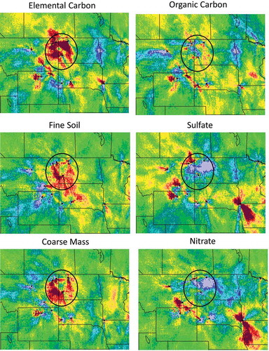
Conversely, there was less likely to be transport from the Bakken area during high-sulfate and -nitrate days during the later time period than the earlier time period. This is consistent with the low sulfur content of the oil and gas in the Bakken region and the decrease in emissions of precursors of these species from coal-fired electric generating stations in the region (see Table 1 and Figure 2). These results are also consistent with the declines in the measured concentrations of these species as shown in Figure 3. The transport difference maps in Figure 6 show a greater likelihood of transport from some areas in Montana, Wyoming, and the Midwest on high-sulfate and -nitrate days during the later years.

High OC concentrations are more likely to originate from parts of the Bakken region in the later years, although the signal is not as strong as for EC, fine soil, and CM. High OC concentrations can be due to emissions from prescribed, agricultural, or wildfires that can vary substantially from year to year (EPA 2016b; Jaffe et al. 2008; Spracklen et al. 2007) or as secondary aerosol from VOC precursor emissions, which have increased substantially in North Dakota (Table 1, Figure 2).

As expected, the results for reconstructed aerosol light extinction (not shown) are very similar to the results for sulfate and nitrate because these two species together make up a majority of the extinction (see Table 3).

Source apportionment estimates

Estimates of the relative contributions to fine particulate matter from regional source areas to measured IMPROVE concentrations are calculated with the Trajectory Mass Balance (TrMB) model (Gebhart et al. 2006, 2011, 2014; Pitchford and Pitchford 1985). This is a receptor technique in which multiple linear regressions are performed using daily concentrations as the dependent variables and corresponding upwind back-trajectory end points in the source regions as the independent variables. When compared with results of other methods, TrMB has been shown to generate reasonable mean source attributions averaged over the time period of the analysis (Gebhart et al. 2006; Pitchford et al. 2005). Because the regression coefficients must account for average emissions, dispersion, deposition, and chemical transformation, it is desirable to minimize the daily deviation of these factors from their means in each regression. For that reason, the TrMB analysis was run separately for each season, with seasons defined as winter (December–February), spring (March–May), summer (June–August), and fall (September–November). The number of observations for each regression must exceed the number of source areas, so to increase the available observations; the seasonal regressions were done as 3-yr averages. For example, the attribution for spring 2014 uses data for spring 2013, 2014, and 2015. Because 2015 was the latest full year for which IMPROVE data were available for this study, the latest year reported for TrMB is 2014. This analysis was completed using three receptor sites in and near the Bakken region, Medicine Lake, Lostwood, and Theodore Roosevelt.

TrMB source areas are shown in Figure 7. Earlier TrMB work (Gebhart et al. 2011) showed that carefully chosen source areas increase the ability of the model to fit the measured data. They were chosen based on several criteria, including first, the interest in the results; in this case, understanding the influence of sources in the Bakken versus those from those outside this area. Second, source areas near the receptor can be smaller than those farther away due to increases in uncertainty of trajectory locations and dispersion as the time between source and receptor increases. Third, model performance is better if most trajectories passing through an area have similar exposure to emissions, dispersion, and chemical transformation en-route to the receptor. Finally, to avoid collinearities between source regions, the timing and number of trajectories passing through each region should be reasonably independent from other regions. For this assessment, source areas were defined to include oil and gas activities (sources 1–7, 9, 10, 22–25), agricultural emissions (sources 7, 8, 11, 13, 15, 16), coal-fired power plants, coal mining (1, 13–17, 21, 22), Canadian oil sands (12), and long-range transport from other urban and industrial areas that are often upwind (17–20, 26). Most source areas have emissions from multiple source types. Because every trajectory must pass through grid cells very near the receptor, and the unchanging temporal patterns are not representative of a time-varying source influence, end points that are very close are eliminated. In previous studies for a single receptor, the source regions themselves were chosen so that they did not include areas close to the receptor. However, for this study using three receptors, we elected to use common source areas for all receptors and remove close-in end points based on either distance or time. The criteria used included eliminating end points within 0.1° or 0.25° of latitude/longitude from the receptor (shown as rectangles around the receptors in Figure 7) or removing end points up to 1, 2, or 3 hr backward from the start time. Rather than attempting to determine the best choices for parameters such as close-in criteria, an ensemble technique (Gebhart et al. 2011) was used in which these criteria, meteorological input data (NARR and NAM12), trajectory lengths (2, 3, and 5 days), season (winter, spring, summer, fall), years (3-yr averages centered on 2002–2014), maximum end-point height (unlimited and top of mixed layer), species (sulfate, nitrate, EC, OC, fine soil, and CM), correlation above which collinear source areas are combined (0.7, 0.8, and 0.9), and receptors (Lostwood, Theodore Roosevelt, and Medicine Lake), were run in all possible combinations, and then the mean results were chosen as best representative of the correct source attribution.

Figure 7. Source areas used in TrMB modeling. Large map shows northwestern United States and southwestern Canada. Inset is western North Dakota and eastern MONTANA as indicated by the guidelines to the larger map. Boxes around the receptors show distances of 0.1° and 0.25° of latitude/longitude.

Detailed annual TrMB results for EC at Lostwood are shown in Figure 8. Each stacked bar shows the source apportionment averaged for all four seasons, with the seasonal results calculated as 3-yr averages centered on the year shown in the x-axis. Source regions in the Bakken are preceded by “BK” in the legend and are at the bottom of the stacked bars in shades of blue for North Dakota or orange for Montana. There was an increase of approximately a factor of 2 in the collective contribution to EC at Lostwood from these sources, with Bakken sources able to account for all of the increase in EC. The growth in influence of the Bakken Northern Wells (source area 3) as the oil and gas activities increased is particularly pronounced. These results and those for EC for Medicine Lake and Theodore Roosevelt are summarized in the top left panel of Figure 9. For all three sites, for both earlier and later years, sources in North Dakota were the largest contributors, accounting for 38–52% of the EC. The biggest change in source attribution for North Dakota sources was seen at Lostwood, where the contribution increased from 38% in the early years to 51% in the later years. Lostwood was also the only site that experienced an increase in mean EC concentration, whereas mean EC at Theodore Roosevelt decreased, and concentrations at Medicine Lake remained relatively constant. These results indicate that receptors closest to the newer active wells were more influenced by oil and gas emissions than those farther south (Theodore Roosevelt) and west (Medicine Lake). The second largest contributor to EC at all three sites was Canada, accounting for 13–32%, with the more northern sites, Medicine Lake and Lostwood, being more influenced by Canada than Theodore Roosevelt. The estimated fraction of EC from Canada remained relatively unchanged in the later years as compared with the earlier years at Medicine Lake, but dropped from 32% to 26% at Lostwood and increased from 13% to 16% at Theodore Roosevelt. The third-largest contributor to EC was Montana, which accounted for 7–13%. EC from Montana decreased at Medicine Lake and Lostwood in the later years compared with the earlier years, while remaining unchanged at Theodore Roosevelt.

Figure 8. Source apportionment results from the TrMB model for EC at Lostwood for 2001–2014. Source names beginning with BK are in the Bakken oil and gas region. Those in blue colors represent North Dakota, reds Canada, pinks midwestern agricultural areas, dark greens Wyoming, oranges Montana, light greens Idaho and Utah, yellows Oregon, Washington, and California. Dashed black line shows the observed concentrations.

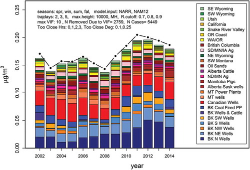
Figure 9. Summarized TrMB source apportionment results for six species for Medicine Lake, Lostwood, and Theodore Roosevelt South Unit for early years (2002–2007) and later years (2008–2014). Arrangement of the species is the same as in Figure 6.

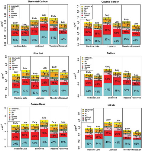
Similar TrMB results are also shown for fine soil and CM in Figure 9. North Dakota sources were the largest contributors to both species at all sites in the later years. In the early years, Canada contributed a larger fraction of CM at Medicine Lake and a larger fraction of both CM and fine soil at Lostwood. North Dakota’s contribution was 33–47% of the fine soil and 29–42% of the CM. The second- and third-largest source regions were usually Canada and Montana, adding 14–34% and 10–18%, respectively. Overall mean concentrations were higher in the later years than in the earlier years for fine soil and CM at Lostwood and Medicine Lake. But mean CM was approximately equal and fine soil decreased at Theodore Roosevelt. The fractional contributions from North Dakota to fine soil and CM increased at all sites, with the drop in mean concentrations at Theodore Roosevelt being mostly due to declines in the contributions from Montana in the later years.

The TrMB model was also run for OC, sulfate, and nitrate (Figure 9). The mean concentrations of these three species declined between the two time periods at all three sites, and the fractional contributions from sources in North Dakota also decreased, except at Theodore Roosevelt, where they increased from 50% to 54% for sulfate and 48% to 53% for nitrate. Conversely, the fractions of these species from Canada increased from earlier to later years, except sulfate at Theodore Roosevelt, where Canada’s contribution decreased from 19% to 16%.

Summary and discussion

Aerosol light extinction or visibility impairment is due to a linear combination of the light scattering and absorption from various types of particulate matter suspended in the atmosphere (Pitchford et al. 2007). In the Bakken area, the dominant contributors to aerosol light extinction are sulfate and nitrate, followed by organic matter, CM, EC, and fine soil. All three analyses, (1) trends in measured concentrations, (2) multisite back-trajectory analysis, and (3) the TrMB source attribution model show that oil and gas activities have had a discernible impact on particulate concentrations in the region. The largest influences were seen on the EC, fine soil, and CM concentrations. Together, these three species accounted for approximately 13–27% of the particulate visibility impairment on average for 2002–2015. The largest impact was at the sites in northwestern North Dakota and northeastern Montana, including Lostwood, Medicine Lake, and Fort Peck, where recent fracking activity has increased the most. The most likely sources of these three species are flaring, disturbed soils, trucking, and construction associated with secondary population growth.

Emissions of SO₂ and NO_x, the precursors to particulate sulfate and nitrate, which are the largest contributors to visibility impairment, have declined during the time period that drilling has increased, with the decline being mostly due to reductions in emissions from coal-fired power plants. This reduction makes it more difficult for receptor-based analyses to discern the impact of the oil and gas emissions on changes in these species. However, the spatial patterns and temporal trends in IMPROVE speciated concentrations showed that during the active period of oil and gas development, sites closest to the Bakken area did not experience the same level of reductions in concentrations relative to other sites in the region, indicating that these species may also be experiencing an impact from oil and gas. The offsetting trends of emission reductions in some species concurrent with increases in others combine to produce a visibility trend in the Bakken region that is not improving as rapidly as in most other areas of the United States.

Acknowledgment

IMPROVE is a collaborative association of state, tribal, and federal agencies, and international partners. The U.S. Environmental Protection Agency is the primary funding source, with contracting and research support from the National Park Service. The Air Quality Group at the University of California, Davis, is the central analytical laboratory, with ion analysis provided by the Research Triangle Institute, and carbon analysis provided by the Desert Research Institute.

Additional information

Funding

This research was funded in part by the National Park Service. The assumptions, findings, conclusions, judgments, and views presented herein are those of the authors and should not be interpreted as necessarily representing official National Park Service policies.

Notes on contributors

Kristi A. Gebhart

Kristi A. Gebhart and is a are research physical scientists in the Air Resources Division of the U.S. National Park Service in Fort Collins, CO.

Derek E. Day

Derek E. Day is a research associate at the Cooperative Institute for Research in the Atmosphere at Colorado State University in Fort Collins, CO.

Anthony J. Prenni

Anthony J. Prenni is an atmospheric chemist in the Air Resources Division of the U.S. National Park Service in Fort Collins, CO.

Bret A. Schichtel

Brett A. Schichtel is a research physical scientist in the Air Resources Division of the U.S. National Park Service in Fort Collins, CO.

J.L. Hand

J.L. Hand is a research scientist at the Cooperative Institute for Research in the Atmosphere at Colorado State University in Fort Collins, CO.

Ashley R. Evanoski-Cole

Ashley R. Evanoski-Cole was a Ph.D. candidate in the Department of Atmospheric Sciences, Walter Scott Jr. College of Engineering at Colorado State University in Fort Collins, CO, and is now an assistant professor in the Department of Chemistry, St. Bonaventure University, St. Bonaventure, NY.

References

- Allen, D. T. 2016. Emissions from oil and gas operations in the United States and their air quality implications. J. Air Waste Manage. Assoc 66 (6):549–75. doi:10.1080/10962247.2016.1171263.
- Ashbaugh, L. L., W. C. Malm, and W. Z. Sadeh. 1985. A residence time probability analysis of sulfur concentrations at Grand Canyon National Park. Atmospheric Environment 19 (8):1263–70. doi:10.1016/0004-6981(85)90256-2.
- Bar-Ilan, A., J. Grant, R. Parikh, R. Morris, G. Heath, V. Diakov, D. Zimmerle, and L. Gribovicz 2015. Moving Towards Improved Basin-level Oil and Gas Inventories and Reconciliation with Measurements: Final report to EPA, 41 pp. https://www.epa.gov/sites/production/files/2015-09/documents/barllan.pdf (accessed April 14, 2017).
- Bar-Ilan, A., J. Grant, R. Parikh, R. Morris, and D. Henderer 2011. Oil and Gas Mobile Sources Pilot Study, Report to EPA, 137 pp. https://www.wrapair2.org/pdf/2011-07_P3%20Study%20Report%20(Final%20July-2011).pdf (accessed August 2, 2017).
- Draxier, R. R., and G. D. Hess. 1998. An overview of the HYSPLIT_4 modelling system for trajectories, dispersion and deposition. Australian Meteorol Mag 47 (4):295–308.
- Evanoski-Cole, A. R., K. A. Gebhart, B. C. Sive, Y. Zhou, S. L. Capps, D. E. Day, A. J. Prenni, M. I. Schurman, A. P. Sullivan, Y. Li, J. L. Hand, B. A. Schichtel, and J. L. Collett. 2017. Composition and sources of winter haze in the Bakken oil and gas extraction region. Atmospheric Environment 156:77–87. doi:10.1016/j.atmosenv.2017.02.019.
- NPS. 2017. Federal Land Manager Environmental Database, Data Exploration, Particulate Matter and Haze Composition. http://views.cira.colostate.edu/fed/SiteBrowser/Default.aspx?appkey=SBCF_PmHazeComp (accessed November 8, 2017).
- Gebhart, K. A., W. C. Malm, M. A. Rodriguez, M. G. Barna, B. A. Schichtel, K. B. Benedict, J. L. Collett, and C. M. Carrico. 2014. Meteorological and back trajectory modeling for the Rocky Mountain Atmospheric Nitrogen and Sulfur Study II. Adv. Meteorol. xx:19. doi:10.1155/2014/414015.
- Gebhart, K. A., B. A. Schichtel, and M. G. Barna. 2005. Directional biases in back trajectories caused by model and input data. Journal Air Waste Manage Association 55 (11):1649–62. doi:10.1080/10473289.2005.10464758.
- Gebhart, K. A., B. A. Schichtel, M. G. Barna, and W. C. Malm. 2006. Quantitative back-trajectory apportionment of sources of particulate sulfate at Big Bend National Park, TX. Atmospheric Environment 40 (16):2823–34. doi:10.1016/j.atmosenv.2006.01.018.
- Gebhart, K. A., B. A. Schichtel, W. C. Malm, M. G. Barna, M. A. Rodriguez, and J. L. Collett. 2011. Back-trajectory-based source apportionment of airborne sulfur and nitrogen concentrations at Rocky Mountain National Park, Colorado, USA. Atmospheric Environment 45 (3):621–33. doi:10.1016/j.atmosenv.2010.10.035.
- Hand, J. L., K. A. Gebhart, B. A. Schichtel, and W. C. Malm. 2012. Increasing trends in wintertime particulate sulfate and nitrate ion concentrations in the Great Plains of the United States (2000–2010). Atmospheric Environment 55:107–10. doi:10.1016/j.atmosenv.2012.03.050.
- Hand, J. L., B. A. Schichtel, W. C. Malm, S. Copeland, J. V. Molenar, N. Frank, and M. Pitchford. 2014. Widespread reductions in haze across the United States from the early 1990s through 2011. Atmospheric Environment 94:671–79. doi:10.1016/j.atmosenv.2014.05.062.
- Hess, A., H. Iyer, and W. Malm. 2001. Linear trend analysis: A comparison of methods. Atmospheric Environment 35:52115222. doi:10.1016/S1352-2310(01)00342-9.
- IMPROVE (Interagency Monitoring of Protected Visual Environments). 2016. Regional Haze Rule Summary data through 1988–2015 (posted December 2016). http://vista.cira.colostate.edu/Improve/rhr-summary-data/( accessed January 9, 2017).
- Jaffe, D., W. Hafner, D. Chand, A. Westerling, and D. Spracklen. 2008. Interannual variations in PM2.5 due to wildfires in the Western United States. Environ. Sciences Technological 42 (8):2812–18. doi:10.1021/es702755v.
- Janjic, Z. I. 2003. A nonhydrostatic model based on a new approach. Meteorol. Atmos Physical 82 (1–4):271–85. doi:10.1007/s00703-001-0587-6.
- Johnson, D., R. Heltzel, A. Nix, N. Clark, and M. Darzi. 2017a. Regulated gaseous emissions from in-use high horsepower drilling and hydraulic fracturing engines. Journal of Pollution Effects and Control. doi:10.4176/2375-4397.1000187.
- Johnson, D., R. Heltzel, A. Nix, N. Clark, and M. Darzi. 2017b. Greenhouse gas emissions and fuel efficiency of in-use high horsepower diesel, duel fuel, and natural gas engines for unconventional well development. Applied Energy 206:739–50
- Malm, W.C., J.F. Sisler, D. Huffman, R.A. Eldred, and T.A. Cahill. 1994. Spatial and seasonal trends in particle concentration and optical extinction in the United States. Journal Geophys Res-Atmos 99 (D1):1347–70. doi:10.1029/93jd02916.
- Malm, W. C., B. A. Schichtel, J. L. Hand, and J. L. Collett Jr. 2017. Concurrent temporal and spatial trends in sulfate and organic mass concentrations measured in the IMPROVE monitoring program. Journal of Geophysical Research - Atmospheres 122 (19):10,462–10476. doi:10.1002/2017JD026865.
- Mesinger, F., G. DiMego, E. Kalnay, K. Mitchell, P. C. Shafran, W. Ebisuzaki, D. Jovic, J. Woollen, E. Rogers, E. H. Berbery, M. B. Ek, Y. Fan, R. Grumbine, W. Higgins, H. Li, Y. Lin, G. Manikin, D. Parrish, and W. Shi. 2006. North American regional reanalysis. Bull. Amer. Meteorol Social 87 (3):343–60. doi:10.1175/bams-87-3-343.
- Murphy, D. M., J. C. Chow, E. M. Leibensperger, W. C. Malm, M. Pitchford, B. A. Schichtel, J. G. Watson, and W. H. White. 2011. Decreases in elemental carbon and fine particle mass in the United States. Atmos Chemical Physical 11. doi:10.5194/acp-11-4679-2011.
- North Dakota Department of Mineral Resources. 2016. North Dakota Drilling and Production Statistics. https://www.dmr.nd.gov/oilgas/stats/statisticsvw.asp ( accessed August 2, 2016).
- North Dakota Department of Mineral Resources, House Appropriations Committee. 2013. https://www.dmr.nd.gov/oilgas/presentations/HouseApprop01102013.pdf (accessed August 2, 2017).
- North Dakota Industrial Commission, Department of Mineral Resources, Oil and Gas Division. 2016. Current Active Drilling Rig List. https://www.dmr.nd.gov/oilgas/riglist.asp ( accessed April 22, 2016).
- Pitchford, M., W. Malm, B. Schichtel, N. Kumar, D. Lowenthal, and J. Hand. 2007. Revised algorithm for estimating light extinction from IMPROVE particle speciation data. J. Air Waste Manage. Assoc 57 (11):1326–36. doi:10.3155/1047-3289.57.11.1326.
- Pitchford, M., and A. Pitchford. 1985. Analysis of regional visibility in the Southwest using principal component and back trajectory techniques. Atmospheric Environment 19 (8):1301–16. doi:10.1016/0004-6981(85)90261-6.
- Pitchford, M. L., B. A. Schichtel, K. A. Gebhart, M. G. Barna, W. C. Malm, I. H. Tombach, and E. M. Knipping. 2005. Reconciliation and interpretation of the Big Bend National Park light extinction source apportionment: Results from the Big Bend Regional Aerosol and Visibility Observational study—Part II. Journal Air Waste Manage Association 55 (11):1726–32. doi:10.1080/10473289.2005.10464766.
- Poirot, R. L., and P. R. Wishinski. 1986. Visibility, sulfate and air-mass history associated with the summertime aerosol in northern Vermont. Atmospheric Environment 20 (7):1457–69. doi:10.1016/0004-6981(86)90018-1.
- Prenni, A. J., D. E. Day, A. R. Evanoski-Cole, B. C. Sive, A. Hecobian, Y. Zhou, K. A. Gebhart, J. L. Hand, A. P. Sullivan, Y. Li, M. I. Schurman, Y. Desyaterik, W. C. Malm, J. L. Collett, and B. A. Schichtel. 2016. Oil and gas impacts on air quality in federal lands in the Bakken region: An overview of the Bakken Air Quality Study and first results. Atmos. Chemical Physical 16 (3):1401–16. doi:10.5194/acp-16-1401-2016.
- Schichtel, B. A., J. L. Hand, M. G. Barna, K. A. Gebhart, S. Copeland, J. Vimont, and W. C. Malm. 2017. Origin of fine particulate carbon in the rural United States. Environment Sciences Technological 51 (17):9846–55. doi:10.1021/acs.est.7b00645.
- Schichtel, B. A., and R. B. Husar. 1997. Regional simulation of atmospheric pollutants with the CAPITA Monte Carlo model. . Journal Air Waste Manage Association 47 (3):331–43. doi:10.1080/10473289.1997.10464449.
- Schwarz, J. P., J. S. Holloway, J. M. Katich, S. McKeen, E. A. Kort, M. L. Smith, T. B. Ryerson, C. Sweeney, and J. Peischl. 2015. Black carbon emissions from the Bakken oil and gas development region. Environ. Sci. Technological Letters 2 (10):281–85. doi:10.1021/acs.estlett.5b00225.
- Seinfeld, J. H., and S. N. Pandis. 1998. Atmospheric chemistry—From air pollution to climate change. New York: John Wiley and Sons.
- Spracklen, D. V., J. A. Logan, L. J. Mickley, R. J. Park, R. Yevich, A. L. Westerling, and D. A. Jaffe. 2007. Wildfires drive interannual variability of organic carbon aerosol in the western US in summer. Geophys. Researcher Letters 34 (16):4. doi:10.1029/2007gl030037.
- Stein, A. F., R. R. Draxler, G. D. Rolph, B. J. B. Stunder, M. D. Cohen, and F. Ngan. 2015. NOAA’s HYSPLIT atmospheric transport and dispersion modeling system. Bull. Amer. Meteorol Social 96 (12):2059–77. doi:10.1175/bams-d-14-00110.1.
- Stohl, A. 1998. Computation, accuracy, and applications of trajectories—A review and bibliography. Atmospheric Environment 32:947–66. doi:10.1016/S1352-2310(97)00457-3.
- Theil, H. 1950. A rank-invariant method of linear and polynomial regression analysis. Proc. Kon. Ned. Adad. V. Wetensch. A 53. 386–392 521-525:1397–412.
- Thompson, T. M., D. Shepherd, A. Stacy, M. G. Barna, and B. A. Schichtel. 2017. Modeling to evaluate contribution of oil and gas emissions to air pollution. J. Air Waste Manage. Assoc 67 (4):445–61. doi:10.1080/10962247.2016.1251508.
- U.S. Environmental Protection Agency. 1999. Regional Haze Regulations: Final Rule, 40 CFR Part 51. Federal Register 64 (126):35714–74.
- U.S. Environmental Protection Agency. 2003. Guidance for tracking progress under the Regional Haze Rule. EPA-454/B-03-004, 96. http://www3.epa.gov/ttnamti1/files/ambient/visible/tracking.pdf (accessed January 23, 2015).
- U.S. Environmental Protection Agency. 2016a. Air Pollutant Emissions Trends Data, State Average Annual Emissions Trend, Criteria pollutants State Tier 1 for 1990–2016. Updated 19 Dec 2016. https://www.epa.gov/air-emissions-inventories/air-pollutant-emissions-trends-data (accessed July 10, 2017).
- U.S. Environmental Protection Agency. 2016b. 2014 National Emissions Inventory, version 1. Technical Support Document, Dec 2016. https://www.epa.gov/sites/production/files/2016-12/documents/nei2014v1_tsd.pdf ( accessed November 7, 2017).
- U.S. Energy Information Administration. 2016. Today in Energy. Natural gas flaring in North Dakota has declined sharply since 2014. https://www.eia.gov/todayinenergy/detail.php?id=26632 ( accessed August 2, 2016).
- Weyant, C. L., P. B. Shepson, R. Subramanian, M. O. L. Cambaliza, A. Heimburger, D. McCabe, E. Baum, B. H. Stirm, and T. C. Bone. 2016. Black carbon emissions from associated natural gas flaring. Environ. Sciences Technological 50 (4):2075–81. doi:10.1021/acs.est.3b04712.