An historical experiment: Los Angeles smog evolution observed by blimp

ABSTRACT

Observations of smog over the Los Angeles Basin (LAB) links high oxidant mixing ratios with poor visibility, sometimes <5 km. By the 1970s, investigators recognized that most of the aerosol affecting visibility was from gaseous oxidation products, sulfate, nitrate, and organic carbon. This led to the 1972–1973 Aerosol Characterization Experiment (ACHEX), which included observations at the ground and from aircraft. Part of ACHEX was the measurement of smog by blimp in a Lagrangian-like format. The experiment on September 6, 1973, demonstrated that a blimp could travel with the wind across the LAB, observing ozone (O₃) and precursors, and particles of different size ranges. These included condensation nuclei (CN) concentrations dominated by particles of ≤ 0.1 µm diameter and light scattering coefficient (b_sc) representing mainly particles of 0.1–2.0 µm diameter. The results indicated a pollutant variation similar to that measured at a fixed site. Ozone was produced in an air mass, reaching a maximum of ~400 ppb in the presence of nitrogen oxides (NO_x) and nonmethane hydrocarbons (NMHCs), then declined. Although the photochemistry was developing, b_sc grew with O₃ mixing ratio to a quasi-steady state at ~9–10 × 10⁻⁴ m⁻¹, decreasing in value much later with decease in O₃. The light scattering coefficient was found to be positively associated with the O₃ mixing ratio, whereas CN concentrations were negatively proportional to O₃ mixing ratio. The blimp experiment was supported with aircraft vertical profiles and ground-level observations from a mobile laboratory. The blimp flight obtained combined gas and particle changes aloft that could not be obtained by ground or fixed-wing aircraft measurements alone. The experiment was partially successful in achieving a true Lagrangian characterization of smog chemistry in a constrained or defined “open” air mass.

Implications: The Los Angeles experiment demonstrated the use of a blimp as a platform for measurement of air pollution traveling with an air mass across an urban area. The method added unique data showing the relationship between photochemical smog chemistry and aerosol dynamics in smog. The method offers an alternative to reliance on smog chamber and modeling observations to designing air quality management strategies for reactive pollutants.

Introduction

As part of the 1972–1973 Aerosol Characterization Experiment (ACHEX), the use of a blimp was explored to conduct a Lagrangian-like air transport study of photochemical smog (Hidy et al. 1974). The experiment was undertaken over the Los Angeles Basin (LAB) on a late summer day that experienced intense photochemical ozone (O₃) levels and aerosol production were intense. The results were not formally published but are described in reports in the archives of the California Air Resources Board (CARB). The results of this study still have potential value for tracing O₃-haze chemistry, although the smog levels are greatly reduced in southern California (e.g., Fujita et al. 2013). The approach remains unique as perhaps the only attempt to observationally trace in a moving, nominal air volume (parcel) photochemical haze pollution from near the Pacific Ocean to the eastern edge of the LAB southeast of the (San Gabriel) mountains.

The blimp experiment traces back to the meteorological surveys of Neiburger and Edinger (1954) and Edinger’s (1973) later series of aircraft flights in 1970. These studies described the daily sea-land breeze structure and the vertical dispersion over the basin, including the marine layer near the ground and a return flow aloft. Air mass trajectory calculations from wind observations of Neiburger, Renzetti, and Tice (1956) provided a background of information on transport and mixing conditions in the subsidence inversion layer over the city. The vertical structure, the mixed and inversion layer relevant to O₃ mixing ratios, was established with Lea’s (1968) research using ozonesonde ascents near Los Angeles. Lagrangian, gas-phase trajectory experiments were conducted later using tetroons (Angell et al. 1972) and helicopters in the 1973 Los Angeles Reactive Pollutant Program (LARPP) (e.g., Eschenroeder, Deley, and Wahl 1973; Feigley and Jeffries 1979). Our experiment was similar in concept to the helicopter-tetroon studies. However, for the first time, we employed the blimp as a carrier for the instrumentation that included measurements of O₃ and its precursors and indicators of size-differentiated aerosol particle concentrations.

In the 1970s, measurements were interpreted with two approaches for developing air chemistry models in urban areas. Modeling at the time was dependent on constraints of computing capability as well as operational computing costs. The first was a chemistry-focused Lagrangian approach for atmospheric processing in air parcels moving in isolation (e.g., the Empirical Kinetics Modeling Approach (EKMA) or Ozone Isopleth Plotting Package (Research Version) (OZIPR) box model Eschenroeder and Martinez 1972; Martinez, Maxwell, and Bawol 1983). The second was an Eulerian approach of averaging chemical reactions in ensembles of air motion moving and intermixing in time across a fixed location (e.g., Urban Airshed Model [UAM]; Reynolds, Roth, and Seinfeld 1973). The former characterized the complex, nonlinear photochemical processes with time without accounting in detail for the added complexities of meteorological processes. The latter modeling adopted similar photochemistry but included simplified meteorology, including winds and mixing, and provided a spatial picture of change with time over an airshed. The Lagrangian calculations represent directly the conditions in air movement. Yet they are difficult to test with observational platforms in ambient air. The Eulerian approach is most amenable to data comparisons from a fixed network of ground stations, but difficult to evaluate aloft from most aircraft observations.

Investigators have known since the 1950s that photochemical smog contains oxidants, mostly O₃, combined with other chemical products, including finely divided aerosol particles. Aerosols identified as haze create severe daytime visibility impairment. Oxidants in smog are associated with the precursors nitrogen oxides (NO_x = NO + NO₂) and (mainly low-molecular-weight) volatile organic compounds (VOCs), a subset of which are nonmethane hydrocarbons (NMHCs) (e.g., Haagen-Smit 1952; Leighton 1961; Renzetti 1959). The origins of haze aerosols are less apparent, even with experiments indicating production of particles from photochemical oxidation of gaseous species in mixtures of sulfur dioxide (SO₂), NO_x, and VOCs (as NMHCs; e.g., Cadle 1973; Leighton 1961; Mader et al. 1952; Renzetti and Doyle 1959).

The CARB was sufficiently concerned about visibility degradation in pollution that it implemented a visibility standard in 1971. The CARB research advisory committee in 1971 believed that a continuous, diurnal observational approach was needed to obtain necessary information about smog aerosols to manage them (and visibility) with oxidant reduction. The ACHEX was organized in response to this need (e.g., Hidy et al. 1980). This experiment ran in the summers and early fall of 1972 and 1973. It was designed to obtain detailed, diurnal gas-particle chemistry, including the spatial and temporal evolution of particle size distributions at a number of sites in California (CA), emphasizing the Los Angeles area. The ACHEX was a derivative of the first experiment to measure gases and particles and optical properties in photochemical smog, the Pasadena, CA, study of 1969 (Hidy 2011; Hidy et al. 1972; Whitby et al. 1972).

The ACHEX was supported with a number of ancillary studies, including a blimp experiment on September 6, 1973, and concurrent meteorological analyses, (fixed-wing) aircraft flights, and special chemical experiments to measure organics in particles, particle water content, and particle formation from VOC oxidation (Hidy et al. 1980). The blimp flight was intended to obtain time-series data for O₃ and precursors aloft along with aerosol indicators in a nominally prescribed air mass in the atmospheric boundary layer over the basin. The blimp was identified as a platform for this experiment for its (a) ability to travel at slow speeds stably at near-constant low heights (cruising speed 50 km/hr), with reduced speed with a vehicle control constraint of less than ~16 km/hr without the vertical or horizontal disturbances associated with helicopter flights; and (b) accessible power and carrying capacity for the aerometric instrumentation. In principle, the former attribute would allow the blimp to travel with an air mass moving across the LAB at low to moderate wind speeds with varying direction. This would represent a quasi-Lagrangian frame of reference for tracing simultaneously photochemical production of O₃ and the aerosol evolution involved in the visual degradation in smog. An Eulerian-like comparison of the blimp results then could be done with aircraft vertical profiles over various locations and observations from the diurnal observations from the ACHEX mobile laboratory.

A well-known feature of smog buildup in the LAB is a persistent sea-land breeze cycle with a strong subsidence (temperature) inversion near the surface. With mountains surrounding the northern and eastern parts of the LAB, the sea breeze is complicated by an evening return flow aloft over the urban boundary layer, “recycling” aged polluted air over the basin (e.g., Blumenthal, Smith, and White 1980; Lu and Turco 1996). The blimp and the (fixed-wing) aircraft observations could account for chemical distributions in the basinwide airflow, enhancing the ability to interpret ground-level data.

The goal of this narrative is to describe the 1973 blimp experiment to link photochemical oxidation to aerosol particle indicators in a moving air mass. The blimp was used for these Lagrangian-like observations of smog, noting the strengths and weaknesses of the method compared with fixed location data. The blimp observations were interpreted for photochemical smog evolution, including oxidant-aerosol relationships and visibility impairment. Although conditions of the 1973 experiment were far more severe for oxidant and aerosol concentrations than seen today, the results and interpretation of the experiment still offer useful information about the air quality optical characteristics in southern California’s photochemical environment.

Methods

Arrangements were made to fly a set of instruments on the Goodyear Company blimp N10A moored in Torrance, CA (Figure S1a). The gondola is shown in Figure S1b. The instrumentation included O₃ and precursers, particle light scattering coefficient (bscat or b_sc) and condensation nuclei (CN), temperature, and relative humidity (RH) (Table S1). Instrumentation was calibrated by standard methods (Hidy et al. 1974). Sampling was conducted with tubes extending from the forward window of the gondola; no specific attempt was made to provide for isokinetic sampling in this flight. The engine mountings are at the rear of the gondola, pointing astern. Since the blimp moves forward for stability, the sampling location should not have been affected by engine exhaust. But this configuration could have distorted sampling of the large (>1.0 µm diameter) particle measurements.

The blimp could fly near the ambient wind speed over the LAB maintaining a constant height in accordance with Federal Aviation Administration (FAA) regulations for aircraft traffic over the city. The blimp needed to maintain control so that its (forward) speed could be sustained at a few km/hr over the ambient airflow. The blimp flight was a Lagrangian-like plan for as far north and east of Torrance as practical, with a return to Torrance from the eastern LAB. A local in-flight test was planned to check the instrumentation in the balloon gondola in the morning of the experiment. After the feasibility of operation was established, a basinwide flight was conducted in the afternoon the same day. The flight strategy was to follow the expected wind trajectories at approximately constant height above the ground within the upper part of the mixed layer. The blimp data were reported as continuous 5-min averages, except for intermittent nitric oxide (NO), temperature, RH, and NMHC observations.

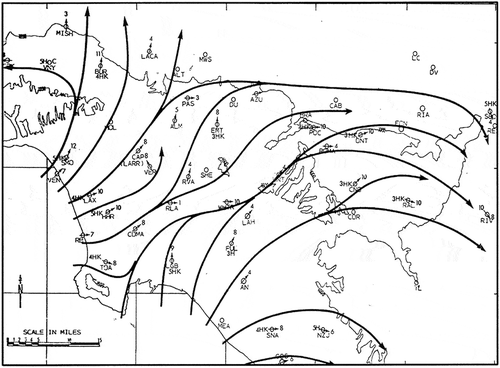
The winds across the basin are approximately the same from day-to-day during this late summer period (e.g., Blumenthal, Smith, and White 1980; DeMarrais, Holzworth, and Hosler 1965). An example of midday streamlines for September 6 is shown in Figure 1. The streamlines reflect the inflow with the sea breeze from the coastal region inland, with a southwesterly flow north of the Palos Verde peninsula, and a convergence near Fullerton (FLA) and a divergence in flow along the San Gabriel Mountains to the north. The westerly component flows east-southeast across the basin past Riverside (RIV) into the desert beyond. The winds crossing the southern part of the LAB enter from the southwest and later curve toward the southeast. After the onset of the sea breeze in mid- to late morning, the air flows in from the coast north to northeast, moving over Torrance towards the mountains, then turns to the east along the mountains towards the desert.

Figure 1. Calculated surface streamlines for midday, September 6, 1973, over the Los Angeles Air Basin. (Calculations from wind data by T. Smith. Source: Hidy et al. 1974.)

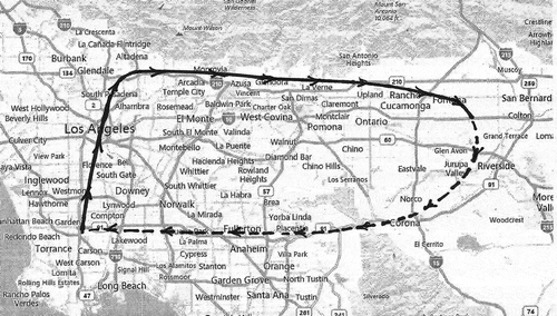
The blimp flight path is shown schematically for the experiment in Figure 2 and in more detail in Figure S2. The times at different parts of the path are included in Table S2 and in Figure S2. The morning test flight (1) is the zigzag pattern north of Dominguez Hills. This flight was used to insure that the instrumentation on the blimp was performing as expected. The afternoon flight (2) is shown in solid arrow pattern with times noted adjacent to flight path. The morning test was done at a height of ~150 m over the nearby Compton industrial area. The afternoon test was designed for a Lagrangian-like travel with an air mass from west to east. In the afternoon, the blimp traveled at ~200–300 m height north-northeast to the San Gabriel Mountains, then turned eastward along the base of the mountains past Asuza and San Dimas to end at the Fontana area. The blimp turned south past Fontana toward Rubidoux, just north of Riverside, then south-southwest to Norco-Corona and westward, traversing the southern basin airflow. The return portion followed the Santa Ana River and the Artesia Freeway from the Norco-Corona area to Torrance. Except for the beginning of the flight over Torrance, the blimp flew near the top of the mixed layer at or just below the temperature inversion throughout the test. During the experiment, entrainment of polluted air from ground level or above the inversion was expected but could not be documented other than qualitatively from turbulence observations and the spatial distribution of source emissions.

Figure 2. Blimp flight on September 6, 1973, originating in Torrance at 1:15 p.m. (PDT). Solid path is the Lagrangian-like section; dashed path is the return to Torrance ending at 6:30 p.m. For additional details, including duration times, see Figure S2 (Hidy et al. 1974).

Instrumented light, fixed-wing aircraft complemented the ACHEX operations (e.g., Blumenthal 2011; Blumenthal, Smith, and White 1980). The aircraft provided vertical profiles of aerometric parameters (Table S1) at several locations across the LAB from near the ground to 1.5 km (5000 ft) altitude. Mixing over the basin was accounted for with aircraft turbulence measurements at each profile site. Spiraling vertical ascents and descents took place over a period limited to several minutes, giving a “snapshot” of conditions. The locations for the vertical profiling by the Naval Weapons Center (NWC) aircraft are noted in dashed ovals in Figure S2. With the exception of Pasadena and the Los Angeles rail yards (LARR), profiles were obtained over airports.

In its transit, the blimp results could be compared with the ground observations. At the eastern end of the eastward trajectory, the blimp flew over the ACHEX mobile laboratory. The trailer was equipped with a range of continuous gas and aerosol particle instrumentation designed to measure the diurnal characteristics of photochemical smog evolution at a series of locations in the LAB (e.g., Sem et al. 2013; Hidy et al. 1980). Measurements at the ACHEX laboratory included continuously measured particle size distributions, particle number and >2-hr average mass concentrations, continuous light extinction and water content, gases (continuous O₃, NO, NO₂, SO₂, carbon monoxide [CO], and multihour canister samples for NMHCs), and continuous meteorological parameters, and analysis for bulk particle chemistry with 2- or 4-hr resolution was conducted off-site as supervised by the California Air and Industrial Hygiene Laboratory. For the blimp experiment, the mobile laboratory was located at Rubidoux just south of Fontana. In the ACHEX design, spatial characterization of air quality data from monitoring across the basin could not be used for the study, since only total 24-hr average total suspended particle (TSP) mass measurements were made with O₃ and sparse NO_x observations.

Results and discussion

With the completed experiment, the collected data were verified for integrity and quality. Aerometric data aloft were analyzed for streamline patterns, vertical cross-sections, and spatial distribution of integrated b_sc with height. Weather conditions for the morning flight on September 6 indicated light winds from the west-southwest to west and temperature in the 20–22 °C range, with early morning fog in the west, but sunny conditions most of the day elsewhere. In the afternoon, the wind speed from the west-southwest increased across the LAB, veering to the east inland, and the temperature rose to the 25–29 °C range. Midday visibility was less than ~8 km, without cloud cover. Winds were in the 15 km range at midday. Later in the afternoon, the winds increased with the sea breeze development across the LAB to a maximum of ~28 km/hr (Hidy et al. 1974).

On the west side, the mid-morning flight over the Compton area experienced weak westerly wind conditions with low O₃ mixing ratio and increasing NO_x mixing ratios, before the late-morning intensification of photochemistry in the LAB. Elevated CN concentrations were observed in the morning, as high as 10 × 10⁴ cm⁻³; b_sc values tended to rise after mid-morning into the 8–9 × 10⁻⁴ m⁻¹ range. By midday, the sea breeze became well organized, with a steady flow inland from the coast toward the San Gabriel Mountains, then eastward into the inland LAB (Figure 1; also examples in Blumenthal, Smith, and White 1980).

The Lagrangian-like portion began at 1:15 p.m. (PDT) in Torrance and ended near Fontana 3:55 p.m. The flight at a near-constant above sea level (asl) profile continued roughly south of Fontana and traveled across the southwesterly airflow in the southern portion of the LAB (Figure 2) and returned to Torrance at 6:30 p.m. The travel time to Pasadena was approximately 1.25 hr, and the travel time from Torrance to Fontana was approximately 2.5 hr. In the eastward part of the flight, the sea breeze carried the blimp inland, ascending through the mixed layer into a layered temperature transition regime, then later mainly into the deepening mixed layer. The blimp trajectory passed over major industrial and commercial areas, with heavy roadway traffic, into more residential areas in a convergence zone west of and around Pasadena where the surface wind slowed at the base of the San Gabriel Mountains.

East of Pasadena the blimp passed over mixed residential and commercial areas toward Fontana, where a large steel manufacturing plant was located. The difference between the rawinsonde and complementary pilot balloon (pibal) observations and the average blimp speed suggests that the blimp moved faster than the wind by ~15 km/hr while traveling eastward across the basin. This was necessary to maintain stability of the blimp during its flight path. The data collected during the afternoon blimp flight are listed in Tables S2 and S3. As the air moved across the LAB, ambient concentrations from source emissions of NO_x and NMHCs (and aerosols) were entrained with ambient O₃ from below and perhaps from above. The loss of species from horizontal and vertical mixing or deposition was not determined. The blimp periodically traveled at a height below the temperature inversion in strong gradients of measured turbulence (e.g., Figures S3–S6). The entrainment of NO_x, NMHCs, and CN from ground emissions was apparent from aircraft data discussed below. As the blimp traveled into the LAB, relative humidity decreased whereas temperature increased eastward from the coast.

The afternoon sequence in Figure 3 shows a well-known photochemical concentration pattern, analogous to a diurnal series, wherein NO_x mixing ratios increased early in the flight when the blimp was over industrial and commercial facilities and heavy traffic sources, later decreasing eastward, whereas O₃ increased to a peak. Measurements of NO in Table S2 suggested that NO_x was mainly NO₂ in the “air mass” tracked by the blimp. NO_x mixing ratios in the flight trajectory were low at the beginning, rising to an initial peak level, then declining until the blimp reached the area approaching and passing south of Fontana. Declines in some of the more reactive components were observed eastward, but the total NMHC levels peaked at Alhambra near downtown Los Angeles. The NMHC/NO_x ratios during the flight are in the order of 1, suggesting a NMHC-sensitive range for the O₃ photochemistry.

Figure 3. Lagrangian-like trajectory observations from the blimp afternoon flight, September 6, 1973. Time series begins at 1:15 p.m. (PDT) at Torrance and ends there at 6:30 p.m. Tabulated data for the experiment are listed in the supplementary material (particle light scattering coefficient is b_sc).

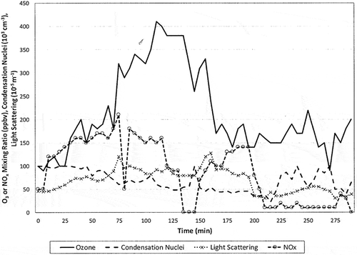
The NO_x increase paralleled O₃ mixing ratio growth in the early part of the flight. Suppression of O₃ mixing ratios with NO titration would have taken place early in the first minute to minutes of flight from Torrance to Pasadena, slowing the rate of O₃ production. Then the growth of O₃ mixing ratio increased rapidly as the blimp moved eastward downwind of Pasadena to Upland, realizing a maximum O₃ mixing ratio reaching 380–400 ppb in the “air mass” from 2:20–2:40 p.m. Ozone mixing ratios then decreased with decline in solar radiation and O₃ loss from the NO reaction or deposition at the ground. After the blimp reached Fontana-Rubidoux area in mid-afternoon, O₃ remained in the 150–200 ppb range through the return flight even though NO sources were present with travel westward. NO_x mixing ratios peaked again on the return leg of the flight. The NO_x series reflects the major source region in the western LAB and from motor vehicle traffic and/or industrial sources. The NMHC species measured during the flight were similar to those found in other LAB studies (Table S4). The data in Table S3 suggest changes in NMHCs eastward along the flight path, with accumulation of relatively nonreactive species early on and later dilution eastward to a minimum near Corona.

The time series from the blimp is reminiscent of species rates of change recorded in smog chamber experiments reported, for example, by Renzetti (1959). The early smog chamber experiments involved high initial concentrations of precursors and constant irradiation but produced a Lagrangian-like evolution of smog chemistry analogous to atmospheric observations. Examples of these results are reported in Renzetti and Romanosky (1956) and Renzetti (1959). These early experiments indicated rapid peaking of O₃ mixing ratios as high as 500 ppb in outdoor air within an hour of irradiation in the chambers. This appears to be similar to the production in the blimp experiment.

Later, Feigley, Jeffries, and Kamens (1982) simulated the evolution of smog chemistry in an outdoor chamber using data from the LARPP. They attempted to account empirically for initial precursor conditions similar to ambient. The tests were followed by periodic precursor injections during the evolution of the chemical processing to account for mixing of ground-level pollution into the mixed layer. One of their experiments included addition of a 1-day carryover of polluted air to simulate mixing of pollution from above the mixed layer. The Feigley, Jeffries, and Kamens (1982) results produced similar chemistry to that observed in a LAB case in early November 1973 obtained from helicopter-tetroon observations tracking airflow. This experiment originated in Downey and later passed northeast through the Puente Hills area south-southwest of West Covina in midday. The maximum O₃ concentration of ~200 ppb achieved in the smog chamber was less than that found in the blimp measurements and occurred in mid-afternoon. Comparison of the blimp results in Figure 3 shows a NO_x peak about an hour into the flight, followed by the O₃ peak ~1.8 hr after the start of the flight. This suggests a more rapid rate of photochemical reactions than projected from the LARPP experiment initiated in the morning.

The blimp experiment illustrates its capability for investigating rate processes in mixing air. For example, the early buildup of O₃ mixing ratio (Figure 3) shows a 2:30 p.m. O₃ production rate of ~200 ppb/hr. This contrasted with a morning O₃ production rate of 30 ppb/hr for a mid-October simulation in Feigler and Jeffries’ smog chamber that was similar to the November helicopter-tetroon operation. The difference between the experiments may be related to the time-of-year, as well as the air mass pathways and the blimp operating height. The blimp experiment traveled 150–200 m higher and well north of the LARPP experiment along the regime known for high oxidant levels compared with conditions further south.

Perhaps the most interesting series in Figure 3 are the CN and b_sc levels compared with the O₃ mixing ratio. The light scattering coefficient is strongly influenced by aerosol volume (mass) in the 0.1–2.0 µm diameter range (e.g., Whitby and Sverdrup 1980), whereas the CN concentrations represent the total number concentration of particles present less than ~0.1 µm diameter. In the experiment, b_sc showed an increase early with O₃, leveling off around Pasadena and later declining at the eastern side of the basin. This increase reflects particle growth as part of the gas-phase processes in smog along with emissions of particles from primary sources. Late in the flight, b_sc lagged the O₃ series decrease, indicating that the presence of photochemically influenced haze remained well after decline of O₃. Indirectly, the production rate of condensed material can be estimated for the growth period in early afternoon. At 1:40 p.m., the b_sc increase early in the flight qualitatively was ~3 × 10⁻⁴ m⁻¹ hr⁻¹. This includes both air chemistry and mixing of ground (primary) emissions or aged aerosols in the air from above.

Using a mass concentration–b_sc relationship from ACHEX ground data (e.g., Gartrell, Heisler, and Friedlander 1980), an estimate of growth in particle mass can be obtained. Their empirical relationship is particle mass (µg/m³) = 33 (b_sc [m⁻¹] × 10⁴ + 0.4). Using this, the estimated 0.1–2.0 µm growth rate early in the flight was ~1.2 µg/m³-min. If ground data analysis of Gartrell, Heisler, and Friedlander (1980) applies to the split, about half of “growth” was emitted “primary” material.

The rapid growth of particles in the 0.1–2.0 µm diameter range early in the flight is attributed to accumulation of low-volatility condensation of products in smog reactions, aside from water vapor absorption, presumably mainly organic material from VOC oxidation or sulfate-nitrate production of oxidation of SO₂ and NO_x (e.g., Gartrell et al. 1980). The NMHC observations of species of carbon numbers >7 were of interest at the time because of particle production but were not measured. Post-1990s evidence suggests that reactive NMHC species having a double carbon bond have the potential to produce particles in a photochemical environment (e.g., Hallquist et al. 2009). From Table S3, there were ample concentrations of reactive NMHC species in the air through C₅ compounds to be available for aerosol growth; the presence of these species likely paralleled the unmeasured high-carbon-number species present at the time.

CN were present in air from the blimp sampling throughout the flight. The CN concentrations were highly variable as found in many urban measurements, including those reported in the ACHEX. The CN concentrations were high at the beginning for the flight and declined as O₃ mixing ratios increased, suggesting the strong influence of primary nuclei sources from combustion and industrial emissions. This is readily seen in the time series of Figure 3 compared with the flight path in Figure 2 (or Figure S2). High concentrations were seen over industrial and high-traffic areas at the beginning of the flight, with a decline as the blimp moved eastward along the less populated mountain slope. Then on the return leg, a rapid increase was seen as the blimp traveled westward towards Torrance in more dense industrial and high-traffic areas after passing across Corona.

Although this experiment provides very limited data from only one flight, the 5-min averaged data give a potentially useful indication of distinctly different relationships between b_sc, CN, and O₃. Data from the time series in Figure 3 show a positive correlation between O₃ mixing ratios and b_sc (for the west-east, Lagrangian-like portion, r = 0.7795; for the entire flight, r = 0.6424), whereas a negative O₃ relation with CN concentration was found (for the west-east portion, r = −0.8932; for the entire flight, r = −0.3113). An approximate linear association between O₃ and b_sc was found to be b_sc (× 10⁴ m⁻¹) = 0.131O₃ + 4.52; R² = 0.610. A relation between O₃ and CN is CN (× 10⁻³ cm⁻³) = −3.3O₃ + 162; R² = 0.464. The relationship between O₃ and b_sc for the blimp trajectory corresponds to evidence of particle growth with photochemical oxidation superimposed on aged particles or direct emissions from sources at the ground.

The series in Figure 3 shows that changes in O₃ and b_sc were coupled at the beginning of the flight and near the end of the eastern leg of the flight. An early plateauing for b_sc developed through most of the Lagrangian-like leg when O₃ was continuing to rise. After O₃ reached a maximum and declined, b_sc declined later in the day following the O₃ decrease. Later in the afternoon, the correspondence in b_sc and O₃ decline was reestablished as air moved into the eastern LAB. This pattern is similar to that observed at the ground during the ACHEX at the fixed site in West Covina (Figure S3; Hidy and Burton 1980). The reason(s) for the plateauing of b_sc with continued increase in O₃ mixing ratio have not been explained. The difference evidently relates to a net ambient condition associated with loss and gain from processes affecting O₃ and b_sc. Ozone concentrations change rapidly with declining sunlight combined with the NO-O₃ reaction.

The afternoon particle net gain or loss in the 0.1–2.0 µm diameter range depends on particle emissions combined with slower growth responding not only to chemical oxidation of precursors but also to humidity and temperature changes, as well as loss by dilution with increasing height of the mixing layer or by evaporation, agglomeration, and surface deposition. The growth of particles in the light scattering size range is dependent on the volatility and hygroscopicity of NH₄NO₃ and accumulating organic material (Collins et al. 2000; Friedlander 1973; Langridge et al. 2012; Seinfeld et al. 2000). How this affects b_sc during the photochemical cycle, with varying precursor emissions and dilution during mixing height increase, is not apparent.

The growth in light scattering infers a relationship with diurnal smog visibility impairment, since b_sc is a major part of the extinction coefficient at ~550 nm wavelength. The light scattering coefficient historically measures a visibility estimate in the absence of light absorption data (e.g., Hidy et al. 1974; White and Roberts 1980). Casual human observations and time lapse photography of the haze over the LAB since the 1950s suggest the connection between O₃ and visibility impairment (e.g., Haagen-Smit 1952). In the absence of fog or low clouds, visibility in the LAB tends to be better in the west along the coast. To the east, smog increases as air dries out inland. Visibility impairment tends to be worse along the San Gabriel Mountains. Movement of the smog follows pollution inland, with the westerly winds maximizing over Upland and reaching the eastern basin and Riverside by mid- to late afternoon. The blimp experiment offered a more quantitative example of visual heterogeneity in smoggy air traveling eastward.

Additional perspective on smog conditions was obtained from the NWC aircraft flights at different LAB locations (small dotted ovals in Figure S2). The vertical profiles were taken by the aircraft ascending and descending in spirals for a sequence of times coincident with the blimp flight (Figure S2; Table 1). The profiles showed both temporal and spatial variations across the LAB, with notable differences in vertical structure complementing changes at ground level. Examples of profiles west to east across the basin are shown in Blumenthal’s original figures (Figures S3–S6), including Torrance, Pasadena, El Monte, and Riverside. Typical of summer LAB conditions, a shallow mixed layer capped by a subsidence layer was found from the ground to about 600 m (~2000 ft). Above this height, temperature tended to rise with strong vertical changes in O₃, CN concentrations, and b_sc. Above the mixed layer, a deep O₃-b_sc layer was evident from aged air remaining as coastal conditions. This layer persisted aloft through the evening into the next day, as inferred by Edinger’s (1973) observations and LAB smog modeling indicated in Lu and Turco (1996).

Table 1. Comparison between blimp observations and aircraft measurements at various locations.

			Blimp				Aircraft
Location	Time PDT	Height (m)^a	O3	bsc	CN	Time PDT	O3	bsc	CN
Torrance	11:33 a.m.	210 (180)	150	5	10	2:07 p.m.	100	5	20
Pasadena	2:25 p.m.	570 (310)	170	7.5	15	2:51 p.m.	200	8	5.5
Junction Hwy No. 19 to No. 210/El Monte	3:00 p.m.	600 (320)	180	7	15	3:13 p.m.	280	6	9.0
Rubidoux/Riverside	4:20 p.m.	630 (250)	300	13	10	4:10 p.m.	200	9.5	3.0
Average			200	8	12.5		195	7.1	9.4

Notes. Tabulated values for O₃ in ppb by volume, b_sc in 10^.4 m⁻¹, and CN in 10⁺⁴ cm⁻³.

^aHeight above the ground; value in parentheses meters asl.

The aircraft data showed a characteristic O₃-particle distribution from the ground to approximately 1500 m (5000 ft) for air parcels over sites at or near the blimp trajectory. Qualitatively, the profiles revealed conditions at blimp height and above, including turbulence in the inversion layers and a turbulence gradient. In and above the mixed layer, there were a range of conditions, including pollutant layering. A few profiles of CO were reported showing apparent well-mixed conditions up to 550–600 m (1800–2000 ft). This was not consistent with b_sc or CN concentrations, which showed gradients through the inversion layer. The elevated CN layers found aloft could derive from the LAB aircraft traffic or could reflect production by nucleation of condensable material. The association between b_sc and O₃ concentrations appeared to be present qualitatively in the profiles up to ~1500 m (5000 ft). The blimp captured the transport and chemistry of O₃, and light scattering changed within the subsidence inversion base across the basin. This evidently was duplicated qualitatively by sampling at a similar altitude the passage of many parcels of air crossing fixed points.

The sequence of aircraft profiles complementing the time series in Figure 3 begins at Torrance (Figure S3) just after blimp launch at 1:30 p.m. The blimp ascended through the marine layer into the subsidence inversion layer where air was sampled in a regime of strong vertical gradients. Above the inversion cap, a layer of elevated O₃ concentration with a CN layer with a maximum concentration at 600 m was observed. The subsidence layer aloft persisted over the LAB during the afternoon as far inland as Riverside. As the blimp traveled northeast over downtown Los Angeles to Pasadena (Figure S4), pollution emissions entered the mixed layer as suggested by high CN concentrations, and b_sc peaked above in the subsidence layer with O₃ below 750 m. The blimp then traveled eastward along the mountains into a regime north of El Monte (Figure S5) where CN maximized near the ground below the blimp height; the blimp encountered strong layering at 150 m with O₃ and b_sc peaking at ~330 m. O₃ and b_sc had a secondary maximum associated with aged air in the subsidence layer at ~670 m. Further inland at Riverside (Figure S6) of the flight, the blimp sampled air showing the highest levels of b_sc, with layering at or above the mixed layer coincident with O₃ layering. Here the temperature profile was nearly isothermal compared with conditions to the west. Above 500 m, weak gradients in species were seen above 700 m. At Riverside, the CO profile showed a gradient from the mixed layer upward to low concentrations in layers coincident with other species.

The aircraft profiles yielded data that are in an Eulerian-like framework, i.e., recording conditions aloft for passage of such a sequence of air parcels over specific locations (Blumenthal, Smith, and White 1980). Conventionally, observers assume that the passage of such a sequence air parcels over a series of fixed sites gives a spatial-temporal picture that is the same as the travel coordinates of a single air parcel. Comparison between the blimp observations and the nearby aircraft observations in Table 1 suggests similarity in results. Averaging the aircraft and blimp observations in Table 1, the two measures are within less than 13%, except for CN, which differs by ~25%. By location, the comparisons are within one another, with a difference of ~30%.

Blumenthal, Smith, and White (1980) found that aircraft profiles for b_sc can be used to construct vertical cross-sections of b_sc versus location for the basin, as shown in Figure S7. Calculated b_sc values are shown for cross-sections across the LAB for midday and for the afternoon on September 6. The cross-sections are qualitatively representative of daytime conditions for b_sc and indirectly variation in visibility impairment in the basin. They infer heterogeneous conditions for visibility impairment, with the severest visibility reduction appearing in the north-central portion of the basin above downtown Los Angeles. The locations of the highest O₃ mixing ratios compare well with the highest b_sc ratio distributions, suggesting the important link between O₃ chemistry and b_sc (Blumenthal, Smith, and White 1980).

The b_sc profiles can also be translated into an integrated light scattering function, with height analogous to an optical depth, as shown in Figure S8. Here the highest optical depth analog is in the north-central part of the LAB, paralleling the highest O₃ levels. Considering September 6 as representative of smoggy conditions in general, one expects that visibility impairment to be most severe along the San Gabriel Mountains eastward. This appears to be the case across the LAB even today.

The ACHEX mobile laboratory was located in Rubidoux, CA, September 5–6. The mobile laboratory sampled air for pollutant gases and particles continuously, 24 hr per day, during the two days. A summary of results from the diurnal measurements is shown in Table 2 for September 6. The table includes meteorological data, pollutant gases, b_sc, and CN concentrations, as well as major chemical components of the aerosol sampled at this location. Other particulate size distributions and air chemistry parameters, including particle composition by size, are not included but can be found in the ACHEX data set (Hidy et al. 1974).

Table 2. Diurnal characteristics of ozone and particles at Rubidoux, CA, September 6, 1973.

Time (PDT)	3:00–8:00 a.m.	8:00–10:00 a.m.	10:00 a.m.–12:00 p.m.	12:00–2:00 p.m.	2:00–4:00 p.m.	4:00–6:00 p.m.	6:00–8:00 p.m.
Wind direction	229	255	248	255	250	238	204
Wind speed (km/hr)	18	11	9.4	11	12.8	7.5	4.5
Temperature (°C)	24	20.6	26.8	20	31	28.4	22.5
RH (%)	100	81	47	31.3	30.5	46.2	77.9
bsc (×10^4 m^−1)	3.83	1.15	8.46	8.68	9.52	9.49	10.9
O3 (ppb)	27.6	69.7	184	200	251	206	134
NOx (ppm)	0.1	0.328	0.104	0.328	0.815	0.965	0.600
CO (ppm)	2.72	3.22	2.08	2.03	2.82	2.51	2.71
CN (×10^−4 cm^−3)	2.3	3.18	4.25	6.21	7.44	6.99	5.81
TF mass^a	87.8	321	268	260	287	306	288
AF mass^b	35.2	67.8	94.8	110	129	116	82.2
TF SO4	6.03	16	20	13.1	24.7	36.7	32.4
AF SO4	2.23	4.89	9.60	8.38	19.6	22.9	13.2
TF NO3	19.2	74.3	76	48.5	73.5	63.6	66.8
AF NO3	7.63	18.1	30	26.5	60.1	30.0	21.2
TF other	62.6	227.3	172	198	179	196	189
AF other	25.3	40.1	55.2	75.1	49.3	33	47.8

Notes. Values averaged over time interval shown. Gas mixing ratios in ppb or ppm by volume. Aerosol mass and components are in µg/m³.

^aTotal filter <20 µm aerodynamic diameter.

^bLundgren impactor after filter <0.5 μm aerodynamic diameter.

The air flowing to Rubidoux in daytime came from west-southwest, with speed peaking with temperature and low relative humidity in the afternoon from 2:00 to 4:00 p.m. Ozone mixing ratios peaked at the same period at 251 ppb, along with b_sc. CN concentrations peaked later with CO in the afternoon between 2:00 and 4:00 p.m. NO_x peaked later at 4:00–6:00 p.m., which was presumably associated with local early evening traffic. The mass concentration of particles <20 µm aerodynamic diameter was very high throughout the day from 8:00 a.m. to 8:00 p.m. The <0.5 µm diameter particle mass concentrations ranged between 20% and 45% of those <20 µm in diameter.

Fine particles sampled in the LAB contain mainly sulfate, nitrate, and carbon species. Sulfate concentrations were high in the ACHEX observations (e.g., Hidy et al. 1980). Nitrate concentrations are unusually high in the eastern part of the LAB. These observations were likely to be only semiquantitative after accounting for known positive and negative artifacts on the filter substrate. High nitrate concentrations are associated with high ammonia emissions to the west from animal husbandry combined with intense photochemical production of nitrates. A multisolvent extraction analysis (Appel, Colodny, and Wesolowski 1980) indicated that, on the average, the particles sampled in 1973, southern California, contained 62% organic carbon and 7% elemental carbon.

Comparison of the blimp and ground-level observations for 4:10 p.m. versus 2:00–4:00 p.m. and 4:00–6:00 p.m. in Table 2 indicates that the O₃ concentrations from the blimp were within the range of ground observations. The light scattering coefficients between the two measures were approximately the same, within <1%. The CN concentrations from the blimp 250 m above ground were much less than at the ground, by more than a factor of 3. This difference is attributed to unmixed CN sources at ground level. The consistency of ground and blimp or aircraft results suggests that in well-mixed conditions, ground measurements can represent data aloft in the mixed layer.

Opportunities for contemporary studies

The Lagrangian-like blimp experiment represents a relatively early attempt to explore the evolution in time of urban gas-phase and aerosol chemistry beyond theoretical applications and modeling. Although limited in scope, the experiment demonstrated that the Lagrangian approach to observing gas-aerosol interactions in the air could guide theoretical advances in an alternative way compared with conventional Eulerian data. Major advantages of experiments in the Lagrangian framework focus on characterizing rate processes in the boundary layer. With its relatively slow speed, the blimp can travel near ambient wind speed such that it could record directly time-dependent processes in smog for both gas and particle chemistry. These would complement aircraft based projects such as those reported by Collins et al. (2000) or Langridge et al. (2012).

There are unresolved contemporary issues about gas and particle chemistry that could be addressed. These include (a) the complexities of nitrogen oxide evolution, associated with the production-loss rates of nitric acid, organonitrates, and particle nitrate; (b) the production of carbonaceous species from atmospheric reactions relative to primary emissions; and (c) the production of CN or ultrafine species of particles compared with primary emissions.

The blimp is capable of flying for considerable distance at low altitude in the mixed layer and into the regime above this layer. The vehicle could be used to look at rate processes extending over distances beyond the scale of the LAB. Using the slow speed and the range of the blimp, the rates and complexities of chemical aging could be traced over a period of a day, including downwind conditions. Investigation of pollution transport from Los Angeles (e.g., Langford et al. 2010) or other large metropolitan areas remains an important issue of pollution management across the West.

Smog visibility impairment remains in issue in the LAB even after major reductions in oxidant precursor and aerosol emissions. There remains a question as to why optical effects have apparently not changed or changed little, depending on location, in the LAB since the 1970s (e.g., Cooperative Institute for Research in the Atmosphere 2006, 2011; La Dochy and Fuentes 1999). Improvements in local visibility from studies evidently are insufficient to characterize the air chemistry changes with optical response. Through experiments by blimp and remote sensing, for example, improvements in knowledge of visual response to smog could be made that at least give the public better understanding of the limits of pollution control on visibility.

Blimp observations could be more efficient and reliable with an engineered package optimizing choices for isokinetic sampling probe mounted, for example, through the windshield. Sampling bias or contamination in the blimp data for different directions relative to the wind is uncertain and would need to be investigated for future use of this aircraft. This capability was not tested in the ACHEX, leaving questions about the actual movement with terrain features. This would be an important test where a three-dimensional effect exists for air moving upwards above a subsidence layer.

Contemporary conduct of Lagrangian-like experiments could adopt not only the blimp platform but also helicopters or even drones. For manned flights, the blimp platform has advantages for conduct of such experiments. Although not documented, the drifting blimp should have minimal effect on surrounding airflow in well-mixed conditions when forward sampling is used. In principle, the blimp can move in the vertical as well the horizontal with the wind to account for vector motion at low speed. The vehicle, with ample power supply, also is capable of carrying relatively heavy instrument payloads. Although drones could be adopted, their carrying capacity would be very limited. Helicopters are an alternative to reach low drift speeds by hovering over a range of heights (e.g., EPA 1979; Feigley and Jeffries 1979). Depending on the helicopter size, it could carry heavy payloads, but it’s not apparent if the aircraft can fly vector (three-dimensional) winds at low speed. Problems exist with the helicopters for potentially modifying the local flow in ambient air. Ambiguities in helicopter applications, for example, are known for sampling because of rotor wash and exhaust around the aircraft and the potential for disturbance in ambient airflow near the aircraft (e.g., Desmet et al. 1995).

The potential for exploiting blimp data for Lagrangian-like studies is limited by its speed to maintain control at altitude. The results are likely to be quantitatively ambiguous with respect to temporal differences in tracking air masses that are entraining emissions and air that has layering within the volume sampled. Modeling or smog chamber experiments simulating the slow-moving aircraft are possible, taking into account time of flight and location. Yet, as a practical exercise, the experiments to date, including the LARPP, have yielded insufficient publication of results on atmospheric processes to support new initiatives for Lagrangian-like experiments. The fixed-site approach still provides a preferred basis for studies that have been key to developing and evaluating models for analyzing urban air chemical processes.

Summary

The blimp flight on September 6, 1973, was the only one of its kind to explore smog photochemistry in a moving air mass over an urban site such as Los Angeles. The height of the blimp flight height was constrained to near constant in the mixing layer, but the blimp experienced a range of polluted air with strong vertical and spatial gradients superimposed on the traveling air mass conditions. The experiment added to knowledge of the following:

1. The experiment explored the feasibility of urban air chemistry for gases and aerosols observations in a Lagrangian-like framework as an alternative to multiple fixed sites.

2. The suitability of a Lagrangian-like study for atmospheric physicochemical rate processes was documented using the blimp platform.

3. Measurements traveling across the Los Angeles area suggested evidence of the relationship between ozone production and optical indexes of haze particles (0.1–2.0 µm diameter), as inferred by observations in an Eulerian framework.

4. Measurements suggested no evidence of an oxidant association with condensation nuclei (ultrafine aerosol) concentrations. The CN levels appeared to be linked primarily with source emissions.

5. The experiment supplied evidence in moving air for heterogeneity of smog haze affecting variation in Los Angeles light scattering and visibility impairment with photochemical processing.

6. The blimp trajectory measurements combined with vertical profiling by fixed-wing aircraft advanced knowledge of gas-aerosol chemistry, air mixing, and air transport in Los Angeles smog that complemented diurnal observations at the ground.

Acknowledgment

In memorium for Don Blumenthal and Ted Smith, then of Meteorology Research Inc., who were major contributors to advancing knowledge of O₃ and aerosol haze aloft in the 1970s and later. Harry Wang guided the blimp and operated the instruments on the blimp flights. Aerosol analyses are from the California Air and Industrial Hygiene Laboratory. The author’s appreciation goes to the Goodyear Company for its participation in the experiment using the blimp platform. The author thanks the U.S. Naval Weapons Center, R. Kelso and P. Owens, for aircraft support; C. L. Blanchard for preparing and editing most of the figures for the manuscript; and the Science Center, Rockwell International, for support of the ACHEX and its special experiments.

Supplemental data

Supplemental data for this paper can be accessed on the publisher’s website.

Additional information

Funding

This project was sponsored as part of the ACHEX by the California Air Resources Board.

Notes on contributors

G.M. Hidy

G.M. Hidy is a principal of Envair/Aerochem. He is a former co-editor of the Journal of the Air & Waste Management Association (JA&WMA).

References

- Angell, J., L. Machta, C. Dickson, and W. Hoeker. 1972. Three dimensional air trajectories determined from tetroon flights in the planetary boundary layer of the Los Angeles Basin. J. Appl. Meteorol. 11:451–471. doi:10.1175/1520-0450(1972)011<0451:TDATDF>2.0.CO;2.
- Appel, B., P. Colodny, and J. Wesolowski. 1980. Analysis of carbonaceous material in Southern California atmospheric aerosols. In The character and origins of smog aerosols, ed. G. Hidy, P. Mueller, D. Grosjean, B. Appel, and J. Wesolowski, 337–350. New York: Wiley Interscience.
- Blumenthal, D. 2011. Measurements of the three-dimensional distribution and transport of aerosols: precedents set by the three-dimensional pollutant gradient study in cooperation with ACHEX. In Aerosol Sci. Technol.: History and reviews, ed. D. Ensor, 297–315. Research triangle Park, NC: RTI Press.
- Blumenthal, D., T. Smith, and W. White. 1980. The evolution of the 3-D distributions of air pollutants during a Los Angeles smog episode: July 24–26, 1973. In The character and origins of smog aerosols, ed. G. Hidy, P. Mueller, D. Grosjean, B. Appel, and J. Wesolowski, 613–649. New York: Wiley Interscience.
- Cadle, R. 1973. Particulate matter in the lower atmosphere. In Chemistry of the lower atmosphere, ed. S. Rasool, 69–117. New York: Plenum Press.
- Collins, D., H. Jonsson, H. Liao, R. Flagan, J. Seinfeld, K. Noone, and S. Hering. 2000. Airborne analysis of the Los Angeles aerosol. Atmos. Environ. 34:4155–4173. doi:10.1016/S1352-2310(00)00225-9.
- Cooperative Institute for Research in the Atmosphere. 2006. Spatial and seasonal patterns and temporal variability and its constituents in the United States. Report IV. Fort Collins, CO: Colorado State University.
- Cooperative Institute for Research in the Atmosphere. 2011. Spatial and seasonal patterns and temporal variability and its constituents in the United States. Report V. Fort Collins, CO: Colorado State University.
- DeMarrais, G., G. Holzworth, and C. Hosler. 1965. Meteorological summaries pertinent to atmospheric transport and dispersion over Southern California. Tech. Paper No. 54.Washington, DC: U.S. Weather Bureau.
- Desmet, G., G. Dumont, D. Tielemans, K. de Lathouwer, and E. Roekens. 1995. Measurement of atmospheric pollutants using helicopters: Evaluation of possible contamination of the sample by turbine exhaust. Atmos. Environ. 29:2547–2552. doi:10.1016/1352-2310(95)00162-R.
- Edinger, J. 1973. Vertical distribution of photochemical smog in Los Angeles basin. Environ. Sci. Tech. 7:247–252. doi:10.1021/es60075a004.
- U.S. Environmental Protection Agency. 1979. The RAPS helicopter air pollution measurement program, St. Louis, MO, 1974–1976. EPA 600/4-79-076. Las Vegas, NV: Environ. Monitoring Systems Laboratory.
- Eschenroeder, A., G. Deley, and R. Wahl. 1973. Field program designs for verifying photochemical models. EPA-R4-73-012c. Research Triangle Park, NC: U.S. Environmental Protection Agency.
- Eschenroeder, A., and R. Martinez. 1972. Concepts and applications of photochemical smog models. In Adv. Chem., Vol. 113, ed. J. Gould, 101–168.Washington, DC: American Chemical Society.
- Feigley, C., and H. Jeffries. 1979. Analysis of processes affecting oxidant and precursors in the Los Angeles Reactive Pollutant Program (LARRP) Operation 33. Atmos. Environ. 13:1369–1384. doi:10.1016/0004-6981(79)90106-9.
- Feigley, C., H. Jeffries, and R. Kamens. 1982. An experimental simulation of Los Angeles Reactive Pollutant Program (LARRP) Operation 33—Part 1. Experimental simulation in an outdoor smog chamber. Atmos. Environ. 16:1989–1996. doi:10.1016/0004-6981(82)90469-3.
- Friedlander, S. K. 1973. Chemical element balances and identification of air pollution sources. Environ. Sci. Tech. 7:235–240. doi:10.1021/es60075a005.
- Fujita, E., D. Campbell, W. Stockwell, and D. Lawson. 2013. Past and future ozone trends in California’s South Coast Air Basin: Reconciliation of ambient measurements with past and projected emission inventories. J. Air Waste Manag. Assoc. 63:54–69. doi:10.1080/10962247.2012.735211.
- Gartrell, G., S. Heisler, and S. Friedlander. 1980. Relating particulate properties to sources: the results of the California aerosol characterization and origins experiment. In The character and origins of smog aerosols, ed. G. Hidy, P. Mueller, D. Grosjean, B. Appel, and J. Wesolowski, 660–713. New York: Wiley Interscience.
- Haagen-Smit, A.J. 1952. Chemistry and physiology of Los Angeles Smog. Ind. Eng. Chem. 44:1342–1346. doi:10.1021/ie50510a045.
- Hallquist, M., J.C. Wenger, U. Baltensperger, Y. Rudich, D. Simpson, M. Claeys, J. Dommen, N.M. Donahue, C. George, A.H. Goldstein, et al. 2009. The formation, properties and impact of secondary organic aerosol: Current and emerging issues. Atoms. Chem. Phys. 9:5155–5236. doi:10.5194/acp-9-5155-2009.
- Hidy, G. 2011. Reminiscences about pasadena, ACHEX and beyond. In Aerosol Sci. Technol.: history and reviews, ed. D. Ensor, 243–265. Research Triangle Park, NC: RTI Press.
- Hidy, G., P. Mueller, D. Grosjean, B. Appel, and J. Wesolowski, eds. 1980. The character and origins of smog aerosols. New York: Wiley Interscience.
- Hidy, G., P.K. Mueller, Y. Tokiwa, and S. Twiss. 1972. Aerometric factors affectng the evolution of the pasadena aerosol. In Aerosols and atmospheric chemistry, ed. G. Hidy, 219–236. New York: Academic Press.
- Hidy, G., K. Whitby, P. Mueller, S.K. Friedlander, B. Appel, R. Charlson, W. Clark, D. Dockweiler, P. Friedman, R. Giauque, S. Green, S. Heisler, J. Huntzicker, K. Kubler, G. Lauer, R. Ragaini, L. Richards, T. Smith, E. Stephens, G. Sverdrup, S. Wall, H. Wang, and J. Wesolowski. 1974. Characterization of aerosols in California (ACHEX), Vol. III. Report SC4524.24FR for the California Air Resources Board. Thousand Oaks, CA: Rockwell International Science Center.
- Hidy, G. and C. Burton. 1980. Atmospheric aerosol formation by chemical reactions. In The character and origins of smog aerosols. ed. G. Hidy, P. Mueller, D. Grosjean, B. Appel, and J. Wesolowski, 385–434. New York: Wiley Interscience.
- La Dochy, S., and D. Fuentes. 1999. Visibility trends in the Los Angeles Basin, 1933-present. WIT Trans. Ecol. Environ. 37. doi:10.2495/AIR990991.
- Langford, A., C. Senff, R. Alvarez, R. Banmta, and R. Hardesty. 2010. Long-range transport of ozone from the Los Angeles Basin. Geophys. Res. Lett. 37:L05807. doi:10.1029/2010GL042507.
- Langridge, J., D. Lack, C. Brock, R. Bahreini, A. Middlebrook, et al. 2012. Evolution of aerosol properties impacting visibility and direct climate forcing in an ammonia-rich urban environment. J. Geophys. Res. 117:D00V11. doi: 10.1029/2011JD017116.
- Lea, D. 1968. Vertical ozone distribution in the lower troposphere near a urban pollution complex. j. Appl. Meteorol. 7:252–267. doi:10.1175/1520-0450(1968)007<0252:VODITL>2.0.CO;2.
- Leighton, P. 1961. Photochemistry of air pollution, 247–253. New York: Academic Press.
- Lu, R., and R. Turco. 1996. Ozone distributions over the Los Angeles Basin: Three dimensional simulations with the smog model. Atmos. Environ. 30:4155–4176. doi:10.1016/1352-2310(96)00153-7.
- Mader, P., R. MacPhee, R. Lofberg, and G. Lawson. 1952. Composition of organic portion of atmospheric aerosols in the Los Angeles area. Ind. Eng. Chem. 44:1352–1356. doi:10.1021/ie50510a047.
- Martinez, R., J. Maxwell, and R. Bawol. 1983. Evaluation of the Empirical Kinetic Modeling Approach (EKMA). EPA/600/3-83/003 (NTIS PB 84128313). Washington, DC: U.S. Environmental Protection Agency.
- Neiburger, M., and J. Edinger. 1954. Summary report on the meteorology of the Los Angeles basin with particular respect to the smog problem. Report 1. Los Angeles, CA: Air Pollution Foundation.
- Neiburger, M., N. Renzetti, and R. Tice. 1956. Wind trajectories of the movement of polluted air in the Los Angeles basin. Report 13. Los Angeles, CA: Air Pollution Foundation.
- Renzetti, N. 1959. Ozone in Los Angeles atmosphere. Adv. Chem. 21:230–282 ed. American Chemical Society Staff, 230-62. Washington, DC: American Chemical Society.
- Renzetti, N., and G. Doyle. 1959. The chemical nature of the particulate in irradiated auto exhaust. J. Air. Pollut. Control. Assoc. 8:293–296. doi:10.1080/00022470.1959.10467856.
- Renzetti, N., and J. Romanosky. 1956. A comparative study of oxidants and ozone in Los Angeles atmosphere. In Paper 56-21. Extended Abstracts, Air. Pollut. Control. Assoc. Annual Meeting, ed. H. Englund, Buffalo, NY, May 20–24, Paper 56-21. Pittsburgh, PA: Air Pollution Control Association.
- Reynolds, S., P. Roth, and J. Seinfeld. 1973. Mathematical modeling of photochemical air pollution—I. Formulation of the model. Atmos. Environ. 7:1033–1061. doi:10.1016/0004-6981(73)90214-X.
- Seinfeld, J., D. Collins, H. Jonsson, H. Liao, R. Flagan, K. Noone, and S. Hering. 2000. Aircraft sampling to determine atmospheric concentrations of particulate matter and other pollutants over the south coast air basin. Contr. Report, 96–315. Sacramento, CA: California Air Resources Board.
- Sem, G., K. Whitby, and G. Sverdrup. 1980. Design, instrumentation and operation of a large mobile air pollution laboratory. In The character and origins of smog aerosols, ed. G. Hidy, P. Mueller, D. Grosjean, B. Appel, and J. Wesolowski, 55–68. New York: Wiley Interscience.
- Whitby, K., B. Liu, R. Husar, and N. Barsic. 1972. The minnesota aerosol analyzing system used in the Los Angeles smog project. In Aerosols and Atmospheric Chemistry, ed. G. Hidy, 189–217. New York: Academic Press.
- Whitby, K., and G. Sverdrup. 1980. California aerosols: Their physical and chemical characteristics. In The character and origins of smog aerosols, ed. G. Hidy, P. Mueller, D. Grosjean, B. Appel, and J. Wesolowski, 477–510. New York: Wiley Interscience.
- White, W., and P. Roberts. 1980. On the nature and origins of visibility-reducing aerosols in the Los Angeles basin. In The character and origins of smog aerosols, ed. G. Hidy, P. Mueller, D. Grosjean, B. Appel, and J. Wesolowski, 716–742. New York: Wiley Interscience.