Reduction of atmospheric fine particle level by restricting the idling vehicles around a sensitive area

ABSTRACT

Atmospheric particles are a major problem that could lead to harmful effects on human health, especially in densely populated urban areas. Chiayi is a typical city with very high population and traffic density, as well as being located at the downwind side of several pollution sources. Multiple contributors for PM_2.5 (particulate matter with an aerodynamic diameter ≥2.5 μm) and ultrafine particles cause complicated air quality problems. This study focused on the inhibition of local emission sources by restricting the idling vehicles around a school area and evaluating the changes in surrounding atmospheric PM conditions. Two stationary sites were monitored, including a background site on the upwind side of the school and a campus site inside the school, to monitor the exposure level, before and after the idling prohibition. In the base condition, the PM_2.5 mass concentrations were found to increase 15% from the background, whereas the nitrate (NO₃⁻) content had a significant increase at the campus site. The anthropogenic metal contents in PM_2.5 were higher at the campus site than the background site. Mobile emissions were found to be the most likely contributor to the school hot spot area by chemical mass balance modeling (CMB8.2). On the other hand, the PM_2.5 in the school campus fell to only 2% after idling vehicle control, when the mobile source contribution reduced from 42.8% to 36.7%. The mobile monitoring also showed significant reductions in atmospheric PM_2.5, PM_0.1, polycyclic aromatic hydrocarbons (PAHs), and black carbon (BC) levels by 16.5%, 33.3%, 48.0%, and 11.5%, respectively. Consequently, the restriction of local idling emission was proven to significantly reduce PM and harmful pollutants in the hot spots around the school environment.

Implications: The emission of idling vehicles strongly affects the levels of particles and relative pollutants in near-ground air around a school area. The PM_2.5 mass concentration at a campus site increased from the background site by 15%, whereas NO₃⁻ and anthropogenic metals also significantly increased. Meanwhile, the PM_2.5 contribution from mobile source in the campus increased 6.6% from the upwind site. An idling prohibition took place and showed impressive results. Reductions of PM_2.5, ionic component, and non-natural metal contents were found after the idling prohibition. The mobile monitoring also pointed out a significant improvement with the spatial analysis of PM_2.5, PM_0.1, PAH, and black carbon concentrations. These findings are very useful to effectively improve the local air quality of a densely city during the rush hour.

Introduction

Atmospheric suspended fine particles (with an aerodynamic diameter ≤2.5 µm, PM_2.5) (Bartell et al. 2013; Langrish et al. 2012; Li et al. 2013) and ultrafine particles (diameter ≤100 nm) (Breitner et al. 2011; Leitte et al. 2011; Liu et al. 2013) are the focus of attention by researchers and others around the world. PM_2.5 is well defined as a heterogeneous mixture of natural and anthropogenic components, including sulfates, nitrates, ammonium, elemental and organic carbon, mineral dust, trace elements, sea salt, pollens, and spores, that has been linked to long-term adverse health effects (Brunekreef and Holgate 2002; World Health Organization 2006; Pope and Dockery 2006). Numerous epidemiological and toxicological studies have demonstrated an association between ambient particulate matter (PM) and cardiovascular and respiratory morbidity and mortality (Bartell et al. 2013; Langrish et al. 2012; Li et al. 2013). Furthermore, the annual deaths caused by PM were estimated to be up to 25% in Ulaanbaatar-Mongolia (Allen et al. 2013).

The physical characteristics of particles (e.g., concentration, particle size, morphology, and porosity) and their chemical characteristics (e.g., composition: ionic components, element or trace metals, organic carbon) are interlinked with atmospheric particle concentrations. It is most likely that a combination of these properties may determine the overall particle toxicity (Hu et al. 2012; Schmid et al. 2007). Furthermore, the various chemical compositions of PM_2.5 might lead to different health risks by the toxic elements and the nonspecific toxicity impact of the particles (Liao et al. 2015; Lu et al. 2016; Saldarriaga-Norena et al. 2009; Wang et al. 2014). Recently, trace metals have been reported as markers to investigate potential emission sources, because they tend to be stable, with low volatility and reactivity in the atmosphere (Hsu et al. 2016). The ionic contents, ammonium (NH₄⁺), nitrate (NO₃⁻), sulfate (SO₄²⁻), sodium (Na⁺), and chloride (Cl⁻), as well as carbonaceous species, elemental carbon (EC) and organic carbon (OC), contents have been reported as the major mass contributors for PM_2.5 around the complex polluted regions of the densely populated cities in east Asia (Hu et al. 2013; Lu et al. 2016; Qin et al. 2015; Tseng et al. 2016).

Nevertheless, mass concentration and number concentration (Liu et al. 2015), as well as particle size distributions, are the main characteristics of PM. These could reflect on source, life time, and physical and chemical properties of PM (Tsai et al. 2015). Source apportionment can further be approached by receptor modeling. There are two widely used methods for this. The first is the Chemical Mass Balance model (CMB8.2), provided by the U.S. Environmental Protection Agency (EPA). The contributions of different sources could be identified by statistical regression after the chemical compositions of PM at receptor sites and from emission sources are analyzed (Chow and Watson 2002; Heo, Hopke, and Yi 2009; Lu et al. 2016; Marcazzan et al. 2003; Watson et al. 2002; Zheng et al. 2002). The other method is to mine the data from long-term or frequently monitored databases, termed positive matrix factorization (PMF), and is effective in analyzing the contributions of sources by multiregression without the demand for source chemical profiles. However, the amount of data should be large enough (suggested to be more than 100) to ensure the accuracy of results (Hsu et al. 2017; Jaeckels, Bae, and Schauer 2007; Okuda et al. 2010; Pandolfi et al. 2011; Sofowote et al. 2015).

Vehicular emissions, industrial exhaust gases, power plants, open burning, and other potential sources are generally indicated as contributors to the PM in the ambient air (Hsu et al. 2017; Liu et al. 2015; Pipalatkar et al. 2014b; Tseng et al. 2016; Wang et al. 2015). Numerous epidemiological studies suggest that exposure sites that have heavy traffic emission–related air pollutants may play a big role in these increased health risks among all sources and that PM is a major contributor in the ambient air. Additionally, the spatial-temporal information is crucial in estimating exposure in a community impacted by roadways, since PM concentrations can vary significantly in both space and time (Karner, Eisinger, and Niemeier 2010; Zhou and Levy 2007). However, studies dealing with measurements on only fixed-site monitoring stations or networks cannot completely capture the spatial variability at small community scales (Han and Naeher 2006). Very local PM emissions, such as from idling operation during vehicle short-parking, might directly affect the health of the people with heart or lung disease, older adults, and children (EPA 2014). Recently, mobile monitoring has become well known in measuring the properties of PM_2.5 and has recently been used to assess exposure with high spatial variability in various geographical settings, using instrumented vehicles (Hagler, Thoma, and Baldauf 2010; Riley et al. 2014; Tunno et al. 2012), bicycles (Pattinson, Longley, and Kingham 2014; Peters et al. 2013; Thai, McKendry, and Brauer 2008), or pedestrians with monitoring instruments (Kaur, Nieuwenhuijsen, and Colvile 2005; Zwack et al. 2011a, 2011b; Rakowska et al. 2014). These studies introduced the advantages of mobile monitoring for investigating the spatial-temporal variations of atmospheric pollutant concentrations. The aim of this research is to evaluate the PM exposure around a primary school in one of the most densely populated areas of Chiayi City, in southern Taiwan.

Both stationary and mobile monitoring approaches are used to measure properties and variations of PM_2.5 before and after the traffic restriction (prohibition of vehicle idling operation). The goals of this study are as follows: (1) to analyze the PM levels, chemical compositions, and contributions from emission sources at the background and campus sites; (2) to identify the hot spots of PM_2.5 and PM_0.1 around the exposure area; and (3) to evaluate the impact on the local air quality by idling restriction of vehicles around a school campus.

Materials and methods

General methodology

The exposure location of this study is an elementary school in Chiayi City, which is a provincial city located in the plains of southwestern Taiwan. It is second densest city in terms of population (4495 people km⁻³) in Taiwan, after Taipei. Operating vehicles in an idling condition emit harmful pollutants into the surrounding ambient air. The nearer points are expected to have higher exposure levels, whereas wind direction also has a major effect on the PM_2.5 dispersion. The roadway in front of the school campus is a potential emission zone, since it is a site where the parents usually drop off and pick up the students, and where vehicles thus idle alongside the road. Therefore, the emission contributors and hot spots should be identified for the students and residents around the school area. The emission rush hour is around two periods, 6:00–8:00 a.m. and 3:00–5:00 p.m., on every school day. In this study, the stationary samplings were designed for analyzing the PM_2.5 mass concentrations, compositions, and source apportionment in the background air and at the campus area. Additionally, a mobile monitoring system was employed for analyzing the spatial variation and mapping the hot spots of PM_2.5 mass and PM_0.1 number concentrations. The air quality impacts were discussed in both normal and after idling restriction cases. The idling prohibition was handled by two inspectors to ensure all the vehicle engines were turned off around the dropping-off/picking-up area during the sampling period.

Sampling strategy

There were two stationary sites, including background and campus sites. The background site was located on the ground about 125 m away from the campus site located inside the school, which was only 5 m away from the dropping-off/picking-up area at ground level (~40 m above sea level), as shown in Figure 1. The wind direction and speed were recorded to support the definition of the above two sites, as shown in Figure 1. The parallel samplings of two stationary sites took place by using time-controllable autosamplers during two periods of idling rush hour on each school day. Each sample collected enough PM_2.5 mass to reach a 24-hr accumulation, meaning that every sample needed six school days to finish a sampling period. There were two periods for each atmospheric condition before and after the traffic restriction.

Figure 1. Sampling sites and wind rose charts around the studied elementary school.

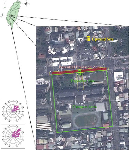
Mobile monitoring was done for 1 hr during the stationary sampling period for each sample, including before and after idling restriction cases. The monitoring area was just around the potential emission area and the campus site (area with yellow dashes in Figure 1) to evaluate the impact on PM hot spots of traffic control. More detailed information about sampling and analyzing processes are described in the following sections.

Sampling and analysis methods for stationary sites

The PM_2.5 sampling method followed National Institute of Environmental Analysis (NIEA) A205, certified by the Environmental Analysis Laboratory (EAL) of the Taiwan Environmental Protection Administration (TWEPA) for each stationary site. The PM_2.5 was collected with two-stage and low-flow-rate ambient air particulate samplers (PQ200 series; BGI, Mesa Laboratories, Inc. Butler, NJ, USA) with a rate of 16.7 L min⁻¹ ± 5% at 1 atm for 24 hr. The particles in the ambient air passed through the inlet unit of the sampler into the first stage of the sampler, a set of very sharply cut cyclones (VSCCs; BGI), to exclude the coarse particles (with aerodynamic diameter >2.5 μm), and PM_2.5 was further captured on the second stage of each filter pack. Each sampling site employed two samplers for parallel sampling in each case. One of them was equipped with polytetrafluoroethene (PTFE; Teflon) membrane filters (diameter: 46.25 ± 0.25 mm) with a Polymethylpentene (PMP) support ring to analyze the particle mass, ionic contents, and metals, and the other was equipped with quartz filters (diameter: 46.25 ± 0.25 mm) for quantifying the elemental and organic carbon in the particles. An electronic microbalance (Mettler Toledo model XP2U) was utilized for determining the mass of sample filters, with sensitivity ±1 μg over a 24-hr period at 23 ± 1 °C and relative humidity at 40 ± 5% in a class 100 clean room. Every filter was weighed two times to ensure the variance was less than 10 μg pre- and post-sampling. The concentration of PM_2.5 was calculated by subtracting the initial mass from the final mass and then dividing by the sampling volume (about 24 m³).

Water-soluble ion analysis

Ion chromatography (IC) was utilized to measure of water-soluble ions, including both anions (Cl⁻, F⁻, NO₃⁻, and SO₄²⁻) and cations (Na⁺, NH₄⁺, K⁺, Mg²⁺, and Ca²⁺), based on the standard procedure from EAL method NIEA W415. The sample was first pretreated; one half of every PTFE filter was shaken in a tube of 15 mL ultrapure deionized water for 30 min and then ultrasonically extracted for 90 min to completely release the species within water-soluble ions. A Ion Chromatography (IC) System (Dionex ICS-1000) with a suppressor (ASRS-ULTRA) and IonPac IC column (AS4A-SC) was used for analyzing the anions, and the other IC (Dionex DX-900) with asuppressor (CSRS-ULTRA) and IonPac column (CS12) using a 0.1 M sulfuric acid (H₂SO₄) eluent was used for analyzing the cations. One blank, one recovery check, and one replicated sample were added to every 10-sample analysis sequence. Deionized water was used as the blank sample, whereas the deionized water solution, composed of 1 mg L⁻¹ standard target ions, was used for calculating the analytical recovery of every ion. The concentrations of blank samples were all lower than the method detection limit (MDL), which was derived from a series of standard solution tests and calculated by the standard deviation of measurements; otherwise, the sample might be contaminated and invalid. The detailed process is introduced in NIEA PA107. The recovery of the analytical method ranged between 85% and 115% in this study. Additionally, the relative percentage difference between the field sample and replication was lower than 20%.

Metal element analysis

Identification of metal elements, including Na, Mg, Al, K, Ca, V, Cr, Mn, Fe, Ni, Cu, Zn, Cd, and Pb, in PM_2.5 was based on EAL method M105. The other half of each of the aforementioned PTFE filters was used for acid digestion. Concentrate nitric acid (HNO₃), hydrochloric acid (HCl), and hydrofluoric acid (HF) in Teflon vessels were used for metal digestion analysis. The metal contents in samples were quantified using high-resolution inductively coupled plasma mass spectrometry (ICP-MS; Jobin Yvon ULTIMA 2000). The calibration curves were evaluated using a standard solution with an absolute error <10%. The recovery of the method was checked every 10 samples by an extra standard sample solution in the range of 75–125%, and the methodological blank sample was determined and found to be less than 2 times MDL. Similar to the ion analyses, the relative percentage difference between the field sample and replicates was less than 20%.

Elemental and organic carbon analysis

The carbonaceous contents (EC, OC, and total carbon [TC]) of PM_2.5 were quantified with an elemental analyzer (EA; Carlo Erba, model 1108). Quartz filters were preheated at 900 °C for 1.5 hr to remove impurities before sampling. The above treatment minimizes the background interference of carbonaceous species originally in the quartz fiber and prevents the overestimation of the EC, OC, and TC from these sources. EA was operated using the oxidation and reduction procedures at 1020 and 500 °C, respectively, by continuously heating for 15 min. Additionally, 1/8 of each quartz filter was heated in advance by nitrogen gas at 340 ± 5 °C for 30 min to expel OC, after which the EC was determined. Another 1/8 of the filter was analyzed without heating, with the carbonaceous contents being considered as total carbon (TC). The amount of OC was then estimated by subtracting the EC from TC. Although thermal analysis is the most widely used method to determine the carbonaceous contents in ambient aerosols, charring can lead to several errors from sample preheating, which were not considered for correction. The above artifacts might result in slightly overestimating EC and further underestimating OC.

Chemical mass balance receptor model

A receptor model, chemical mass balance (CMB), was utilized to determine the contributions of various sources that had potential effects in the exposure area. The chemical compositions of PM_2.5, including measurements from in previous studies and from receptors sampled in this study, were the input of the CMB model. Previous researchers have noted that this kind of method was used in the early 1970s and that the model needs to collect samples at the receptor field in order to quantify the chemical species presented in the emission sources. The CMB model starts with a matrix of linear equations that expresses each set of PM_2.5 chemical contents measured in the atmosphere at the ambient site by the sum of products of source contributions and compositions. The possible sources and their properties can be less than the number of determined species (Hanzel and Durham 2005; Watson et al. 1994). An equation of mass balance is as follows (eq 1):

(1)

where C_i is the concentration of species (i measured at the receptor site in µg m⁻³); a_ij is the mass fraction of species (i in the profile of the source j); n is the number of species; and S_j is the mass concentration at the receptor site of overall species assigned to the source j (µg m⁻³).

There are some assumptions used in the CMB model, as follows: (1) the compositions of the emission sources stay in a constant state during the sampling period; (2) there is no interchemical reaction among the species; (3) all sources should be identified; (4) the amount of chemical species is more than the sources; (5) the source profiles are linearly independent; and (6) if any other ambiguities are disassociated, then they are normally distributed (Watson et al. 1994).

Spatial analysis for PM_2.5 and PM_0.1 by mobile sampling system

The mobile sampling method was also applied in this research, using an electric-powered tricycle carrier (Figure 2), as introduced in other previous research (Berghmans et al. 2009; Pattinson, Longley, and Kingham 2014; Peters et al. 2013; Thai, McKendry, and Brauer 2008). The mobile system is equipped with a global positioning system (GPS), two particle monitors (DustTrak and an P-TRAK), a photoelectric aerosol sensor, and a microAeth.

Figure 2. The tricycle carrier used for the mobile monitoring system in this study.

The GPS used in this study was produced by Garmin. The PM_2.5 mass concentration was monitored by a DustTrak (DustTrak 8530; TSI) along the pathway of the mobile monitoring system. The measurable aerodynamic diameter ranged from 0.1 to 10 μm, when the sampling flow rate was 3 liters per minute (Lpm). The real-time data were recorded every second with the detection concentration ranging from 0.001 to 400 mg m⁻³. The DustTrak used in this study was calibrated by the PQ200 sampler employed by the TWEPA stationary site for 7 days. The regression equation was then used to transform the DustTrak data into more comparable ones. Ultrafine particle number concentration was monitored by a P-TRAK (PTRAK 8525; TSI) in this study. The 0.001–0.1 μm size range could be monitored with 0–500,000 cm⁻³. The sampling flow rate was 0.7 Lpm, when each real-time data were collected every second.

Polycyclic aromatic hydrocarbons (PAHs) were also monitored by a photoelectric aerosol sensor (PAS; PAS2000; EcoChem Analytics). The detection concentration ranged from 0.3 to 1.0 g m⁻³ with a 2 L min⁻¹ constant sampling flow rate. The ambient PAH levels were recorded once every 6 sec. BC monitoring was done by the fourth device on the mobile system, the microAeth. The detection range was 0–1 mg BC m⁻³, whereas the resolution was ±0.001 μg BC m⁻³.

The mobile monitoring system could record the location, PM_2.5 mass, PM_0.1 count, PAH mass, and BC mass information simultaneously. Every mapping mission was done during 1 hr and neglected the slight time variations of air quality and weather conditions during the monitoring hour. MATLAB R2014a (MathWorks, Natick, MA, USA) was utilized to carry out the statistical analysis. The data from each monitor were first checked by a Kolmogorov-Smirnov normality test, and further analyses of the differences between traffic-restricted and nonrestricted cases were done using a Kruskal-Wallis test to identify their significance.

Results and discussion

Atmospheric levels of PM_2.5 on potential emission zone

The atmospheric PM_2.5 profiles are shown in Figure 3. Both the background and campus sites were analyzed both before and after the idling restriction. As seen in the figure, the concentration of PM_2.5 before idling restriction exceeded the World Health Organization (WHO) guideline (25 μg m⁻³) at both the background and campus sites (Tseng et al. 2016). However, more information is needed in order to understand if the idling restriction is the appropriate way to control the emissions surrounding the elementary school. In comparison, the atmospheric PM_2.5 mass concentration at the campus site was 47 μg m⁻³, which was 15% higher than that at background site (54 μg m⁻³) before the idling restriction, when the ions were the major content of PM_2.5, among others, including metal and carbon groups. Moreover, the exposure level was 44 μg m⁻³, representing only a slight 2% increase compared with that at the background site (45 μg m⁻³) after the idling restriction was implemented in the exposure area. Obviously, the increase in PM_2.5 from the background site to the campus site was mainly contributed by water-soluble ions, whereas the rest of the components did not have significant effects. This reveals that any control strategy must address ion control of the PM_2.5 composition, after the source apportionment is done.

Figure 3. Atmospheric PM_2.5 mass concentrations and major chemical compositions around an elementary school before and after the restriction of vehicle idling operation.

Ionic composition in the potential emission zone

In order to confirm that the emission control of idling vehicles was a proper and effective strategy, the fractions of individual ionic compounds in PM_2.5 at the stationary sites were evaluated, as shown in Figure 4. The three major ionic components were nitrate (NO₃⁻), sulfate (SO₄²⁻), and ammonium (NH₄⁺), which represented 47.0%, 25.6%, and 20.5% of the mass of total ions in PM_2.5, respectively, at the campus site. Meanwhile, their contributions approached 41.4%, 27.7%, and 23.4%, respectively, in the background air before the prohibition of idling vehicles. After idling restriction, the fractions of NO₃⁻, SO₄²⁻, and NH₄⁺ at the campus site were reduced to 31.0%, 38.5%, and 27.1%, respectively, whereas they were 32.2%, 38.4%, and 25.8%, respectively, at the background site. These results are similar to those of a previous study that found that the amount of cations will be higher in summer, autumn, and winter but lower in spring, in contrast to the findings for anions in Chiayi City. The anion-to-cation ratio in this study ranged from 0.80 to 1.11, which indicates that the ions were balanced to form ionic particulate contents from secondary aerosols (He et al. 2012; Tseng et al. 2016).

Figure 4. Ionic compositions of the atmospheric PM_2.5 around an elementary school before and after the restriction of vehicle idling operation.

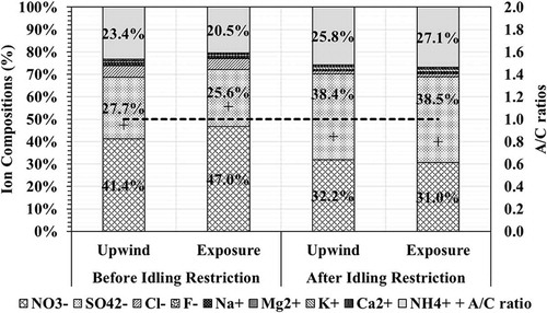
Before the idling restriction, there were different compositions among ions at the campus site from those at the background site, and these differences between the two places disappeared after the idling restriction was implemented (Figure 4). Furthermore, as the ion contents increased in Figure 3 as well as the NO₃⁻ in Figure 4, the NO₃⁻ might be the major problem that has a significant role within PM_2.5 in the potential emission zone, which in this study was subject to a restriction to control the behavior of parents with regard to using vehicles around the school area. However, the NO₃⁻ in the ambient air might not only come from the exhaust gas of vehicles, as emission standards are now becoming more stringent, and they were possibly emitted from a source of other transported emissions. Lin reported that the higher NO₃⁻ and SO₄²⁻ compositions significantly increased through the atmospheric oxidation process from the NO, NO₂, and SO₂ emitted from various sources, including boiler plants, factories, or even from airborne reactions (Lin 2002). Other previous studies have claimed that NO₃⁻, SO₄²⁻, and NH₄⁺ are the major contributors of water-soluble ions in particles (Deshmukh et al. 2011; Lu et al. 2016; Shen et al. 2009; Wang et al. 2015). As such, we have conducted more data analyses to support the idea that the idling restriction was working to reduce the PM_2.5 levels around the school hot spot.

The sulfur oxidation ratio (SOR) and nitrogen oxidation ratio (NOR) were used to understand how much sulfur compounds and nitrogen compounds are able to neutralize NH₄⁺. SOR and NOR are derived from eqs 2 and 3, respectively:

(2)

where nss．SO₄²⁻ is the concentration for non-sea-salt SO₄²⁻ in ambient air (μg m⁻³); nss．SO₄²⁻ = SO₄²⁻ − 0.251 × Na⁺; and SO₂ is the concentration of SO₂ in gaseous phase (μg m⁻³).

(3)

where NO₃⁻ is the concentration for NO₃⁻ in particulate phase (μg m⁻³) and NO_x is the concentration for NO₂ in gaseous phase (μg m⁻³).

As shown in Table 1, the SOR and NOR values have been investigated in Taiwan from 2006 until 2013, which correlates with this study. SOR and NOR values before the idling restriction were 0.582 and 0.184 in the background air and reached 0.605 and 0.233 at the campus site, respectively. After the idling restriction, reductions in SOR and NOR were found in both places, when their levels reduced to 0.505 and 0.167 at the background site and 0.502 and 0.160 at the campus site. The NOR value was always smaller than the SOR value in both places and under both conditions. Previous studies have speculated that low levels of SOR or NOR indicate less potential secondary aerosol formation (Tseng et al. 2016). The small amounts in the current study might be due to local emissions.

Table 1. Comparison of SOR and NOR values of the studied elementary school in this research and the ambient sites reported in the literature.

Sampling site	Site properties	Condition	SOR	NOR	Reference
Elementary school	Before idling restriction	Background	0.582	0.184	This study
		Exposure	0.605	0.233
	After idling restriction	Background	0.505	0.167
		Exposure	0.502	0.160
Ambient air	Yunlin (rural)	Autumn	0.370	0.180	Lin 2013
	Yunlin (urban)	Autumn	0.450	0.190	Jung 2010
	Chiayi (suburban)	Autumn	0.320	0.034	Lin 2013
	Chiayi (suburban)	Autumn	0.450	0.190	Jung 2010
	Tainan (urban)	Spring	0.250	0.080	Tsai 2011
	Tainan (urban)	Winter	0.360	0.130	Tsai 2011
	Kaohsiung (industrial area)	Spring	0.320	0.050	Yu 2003
	Kaohsiung (urban)	Spring	0.420	0.110	Yu 2003
	Pingtung (urban)	Summer	0.300	0.090	Chiang 2007
	Pingtung (suburban)	Spring	0.490	0.040	Yu 2003
	Pingtung (suburban)	Winter	0.360	0.100	Tsai 2006

In ambient air, NH₄⁺ has a neutralizing function on NO₃⁻ and SO₄²⁻, whereas their equivalent ratios in aerosol indicate different neutralizing states. In the environment, these three main ionic components should formulate different salts in PM_2.5 as NH₄NO₃, NH₄HSO₄, and (NH₄)₂SO₄, and so on (Steinfeld 1998). The amount of ammonium determines how much contradictive agent could be neutralized (Tseng et al. 2016). I and J values indicate how far the neutralization process is ideally allowed. Index I is equal to the equivalent mole ratio of NH₄⁺ and SO₄²⁻ in the aqueous phase, as shown in eq 4. There is NH₄SO₄ presented when I > 2.0, partial NH₄HSO₄ presented when I < 2 (Chu 2004). Index J is equal to the equivalent mole ratio of NH₄⁺ over the sum of sulfate and nitrate (2SO₄²⁻_eq + NO₃⁻_eq), as shown in eq 5, meaning that NH₄⁺ is sufficient to neutralize NO₃⁻ and SO₄²⁻ when J is equal to or greater than 1.0 (Tseng et al. 2016).

(4)

(5)

The ion concentration results were further calculated for the I and J values, as shown in Figure 5. I was greater than 2.0 and J was greater than 1.0 at the background site before idling control took place, meaning that most of the sulfates and nitrates were balanced to form fine particles. There is rich NH₄⁺ from the potential sources of fermentation products of agricultural waste and plant decomposition, livestock operation, biomass burning, and natural soils around southern Taiwan. On the other hand, I was greater than 2.0 and J was less than 1.0 at the campus site before the idling restriction, indicating that most of the sulfates were balanced but not the nitrates. Additionally, the transformation rate from SO₂ to SO₄²⁻ was significantly higher than from NO₂ to NO₃⁻. Therefore, the nitrogen oxide (NO_x) emission controls could be more effective in inhibiting the secondary fine particle formation and reduce the local PM_2.5 level.

Figure 5. I and J values of the atmospheric PM_2.5 around an elementary school before and after the restriction of vehicle idling operation.

Metal and carbonaceous species in atmospheric PM_2.5 around exposure area

Chemical composition analysis is one way to determine whether the emissions were coming from local traffic emissions or from other transported emissions. Metal composition was used as a fingerprint of the PM_2.5 collected at each site around the elementary school before and after restrictions, as shown in Figure 6. The concentrations (in percentage) are in the order Na > K > Fe > Mg > Al > Zn > Ca > Pb > Ba > Mn > Cu > V > Cr > Ni > Mo > Sr > Ti > Sb > As > Li > Rb > Cd > Pt. Some compounds represent sea salt components, whereas others include soil dust, boiler combustion, open burning, and factories (Pipalatkar et al. 2014a, 2014b, ; Tseng et al. 2016).

Figure 6. Atmospheric PM_2.5 mass concentrations and major chemical compositions around an elementary school (a) before and (b) after the restriction of vehicle idling operation.

Before the traffic restriction, most of the species increased from the background site to the campus site, including Fe, Mg, Al, Zn, Ca, Ba, Cu, V, Cr, Ni, Sr, Ti, and Sb. This might be because of the near-surface emissions (traffic, road dust, boiler, catalyst, and cooking) from the densely populated city surrounding the school area. A different trend was found after the idling restriction, with the anthropogenic species (Zn, Pb, Ba, Mn, Cu, V, Cr, Ni, Ti, and Sb) in PM_2.5 reduced and the crustal elements (Na, Mg, Al, and Ca) increased, as shown in Figure 6. The effects of traffic control were again supported by this observation.

The contributions of the EC and OC, as well as the TC content in the PM_2.5 and the OC/EC ratio, are shown in Table 2. The EC, OC, and TC levels were 3.35, 6.03, and 9.38 μg m⁻³, respectively, at the background site and increased to 4.52, 7.59, and 12.1 μg m⁻³, respectively, at the campus site before the traffic restrictions. The larger difference between the two sites was narrowed down after the idling emissions were inhibited. Previous studies have reported that a ratio of OC/EC above 2.2 or an OC/TC value over 0.67 indicates the generation of the secondary carbonaceous aerosol (Turpin and Huntzicker 1995). In the current study, the OC/EC ratios were all below 2.2, representing a typical atmospheric PM_2.5 condition of a densely populated area with a heavy traffic (primary emission) load. Nevertheless, the OC/EC ratio decreased from 1.80 at the background site to 1.68 at the exposure area, indicating that there might exist several local primary sources of carbonaceous species. This condition was eased after inhibiting the traffic emissions, which led to OC/EC ratios of 2.03 and 2.12 at the background and campus sites, respectively.

Table 2. Comparison of secondary organic carbon levels at the studied elementary school and the ambient sites reported in the literature.

Sampling site	Site properties	Condition	Carbonaceous species	SOCmin/OC	Reference
Elementary school	Before idling restriction	Background	EC: 3.35 μg m^−3 OC: 6.03 μg m^−3 TC: 9.38 μg m^−3 OC/EC: 1.80	11%	This study
		Exposure	EC: 4.52 μg m^−3 OC: 7.59 μg m^−3 TC: 12.1 μg m^−3 OC/EC: 1.68	4%
	After idling restriction	Background	EC: 3.51 μg m^−3 OC: 7.17 μg m^−3 TC: 10.7 μg m^−3 OC/EC: 2.03	21%
		Exposure	EC: 3.59 μg m^−3 OC: 7.59 μg m^−3 TC: 11.2 μg m^−3 OC/EC: 2.12	24%
Ambient air	Chiayi (urban)	Summer	—	22%	Chang-Chien 2014
	Chiayi (urban)	Autumn	—	6%	Chang-Chien 2014
	Chiayi (urban)	Winter	—	4%	Chang-Chien 2014
	Taipei	Spring	—	4%	Lee et al., 2012
	Taichung	Spring–autumn	—	15%	Chou 2006
	Nantou	Spring–autumn	—	18%	Chou 2006
	Tainan (urban)	Winter	—	13%	Tsai 2006
	Kaohsiung (industrial area)	Winter	—	19%	Chen 2006
	Pingtung (urban)	Summer	—	65%	Chiang 2007
	Pingtung (suburban)	Autumn–spring	—	43%	Chen 2006

Secondary organic carbon (SOC) is another index to identify the products from secondary atmospheric photochemical reactions (Zhang et al. 2012), which was determined using the equation proposed by Castro. The minimum OC/EC ratio during the sampling period was used as a good primary OC tracer and an indicator of anthropogenic pollutants (Castro et al. 1999; Huang et al. 2014; Zhang et al. 2012). The equation proposed by Castro has the following form (eq 6):

(6)

where SOC is the concentration of secondary OC (µg m⁻³), OC_total is the total concentration of OC (µg m⁻³), (OC/EC)_min is the OC/EC ratio at the minimum level in the ambient air during the sampling period, and EC is the elemental carbon compound (µg m⁻³).

Furthermore, the SOC values in Table 2 are also comparable to those found in previous studies. In this research, the SOC value reached 11% at the background site and 4% at the campus site before idling restriction, supporting the trend found in the OC/EC ratios. Furthermore, the SOC had similar contributions of 21% and 24% of the mass on total carbonaceous species at the background and campus sites after idling restriction, indicating that the effects of local emission had been reduced. Similar results were also found in a prior study, where the lower SOC value in Chiayi City was probably caused by a high value of EC composition, which is well known as black carbon (BC) and emitted by the surrounding local traffic (Tseng et al. 2016).

PM_2.5 source apportionment

The CMB model is one of the most promising models that are often used for calibrating the contributions from emission sources by carrying out metal, ion, and carbon fingerprint analyses. In this study, the subjects were classified by the major emission sources, as shown in Figure 7, including mobile (MO), waste incinerators (WI), metallurgical industry (MI), petrochemical industry (PI), agricultural burning (AB), and boilers and furnaces (BF); for the source profiles, refer to our previous studies (Hsu et al. 2016; Lu et al. 2016; Tseng et al. 2016). These are six major sources contributing to the atmospheric PM_2.5 at the background site, including mobile sources (MO; 36.2–37.6%), secondary sulfate (22.1–23.2%), secondary nitrate (7.4–8.7%), organic carbon (OC; 5.6–9.3%), and metallurgical industries (MI; 2.9–4.4%). Figure 8 shows the results of 12-hr inverse trajectories of regional sources and the transport of air pollutants that might impact the air quality at the target area in this study. For the before traffic restriction case, the airflow originated from Taoyuan in northern Taiwan passed through the Hsinchu industrial area, Taichung City, Taichung port, a coal power plant, and further went through the agricultural area in Changhua and Yunlin counties, and again passed through a small petrochemical industrial area at the north of Chiayi City, and finally entered the focal school area (as shown in Figure 8a). The contributions of these complicated emission sources could be found in the CMB results, as seen in the background atmospheric PM_2.5 composition of Chiayi City during the sampling period.

Figure 7. Source contributions evaluated by CMB model around the studying elementary school before and after the restriction of vehicle idling operation. MO = mobiles; WI = waste incinerators; MI = metallurgical industry; PI = petrochemical industry; AB = agricultural burning; BF = boilers and furnaces.

Figure 8. Inverse trajectory modelings of the atmosphere around the studying elementary school (a) before and (b) after the restriction of vehicle idling operation.

Notably, the mass contribution of mobile sources increased to 42.8%, whereas the organic carbon content reduced to only 5.4% in the base condition without any traffic control. This phenomenon might be due to the local emissions of passenger cars and idling vehicles, which produce heavy primary black carbon and soot, increase EC content, and subsequently reduce the contribution of OC (Chen et al. 2017; Turpin and Huntzicker 1995). On the other hand, the MO contribution reduced to a normal level (36.7%) at the campus site, which was similar and even lower than that of the background site (37.6%) after the idling restriction. Therefore, the above results strongly support the idea that the prohibition of all idling of vehicles near the school area could effectively reduce the local PM_2.5 emissions and exposure of students, parents, and residents. However, the petrochemical industries (PI) contributed 7.1–8.6% in the second sampling period by mid-term transport, even though the traffic was well controlled. Figure 8b shows the historical pathway of the airflow at the campus site after the idling restriction, which originated from the Taiwan Strait, and passed through a large-scale petrochemical industrial area (coal power plant, stacking field, port, and ship emissions were included), farm fields in Yunlin and Chiayi counties, and a small petrochemical area at northwestern Chiayi City. The international or intercounty transport might be hard to eliminate. Therefore, the control strategy for local emission sources is both more important and effective.

Evaluating the effects of idling restriction by mobile pollution monitoring

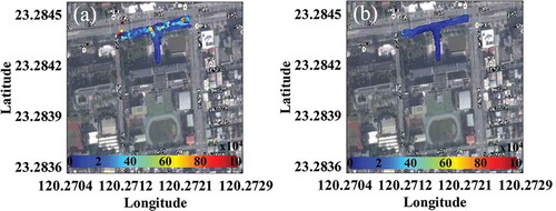
PM_2.5 (μg m⁻³), PM_0.1 count (cm⁻³), PAHs (ng m⁻³), and BC (ng m⁻³) were then monitored around the roadside and into the front door of school campus. The PM_2.5 DustTrak results were calibrated by the PQ200 manual particle sampler installed in the EPA Chiayi site to keep all the PM_2.5 data based on the same measurement technique. PM_2.5 mass concentrations around the school are shown in Figure 9. The intensity along the roadside and front door area ranged from 40 to 100 μg m⁻³ before traffic prohibition. Most of the PM_2.5 levels were around 40–60 μg m⁻³, similar to the normal level in a densely urban area; meanwhile, several red dots (80–100 μg m⁻³) occurred at the front door of the school and at the eastern intersection, indicating that the idling vehicle emissions were an even higher contribution than normal traffic emissions to the hot spot during the sampling period. The PM_0.1 number concentrations ranged from 2 × 10⁴ to 10 × 10⁴ cm⁻³, as shown in Figure 10. The hot spots existed along the road, since the vehicles might have a stronger potential to emit fine and ultrafine particles than the other emission sources (Burtscher 2005; McCreanor et al. 2007; Zhu et al. 2002). The results became impressive, as the hot spots disappeared and the atmospheric PM_2.5 and PM_0.1 concentrations decreased to the range of 20–60 μg m⁻³ and 2–4 × 10⁴ cm⁻³ after the policy was applied. Idling vehicles have been proven to be a potential emission source that has an important impact on the concentration of PM_2.5 in microscale ambient air around sensitive areas.

Figure 9. Spatial analysis of PM_2.5 mass concentrations (a) before and (b) after the restriction of vehicle idling operation.

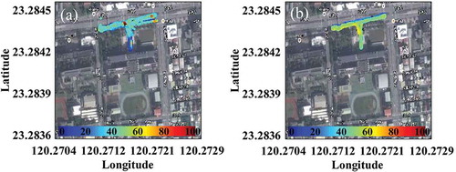
Figure 10. Spatial analysis of PM_0.1 count concentrations (a) before and (b) after the restriction of vehicle idling operation.

The overall statistically significant results during 1-hr mobile monitoring are reported in Table 3. The average levels of PM_2.5, PM_0.1, PAHs, and BC were 53.9 μg m⁻³ (n = 3594), 3 × 10⁴ cm⁻³ (n = 3594), 25 ng m⁻³ (n = 700), and 2890 ng m⁻³ (n = 474), which were significantly reduced by 16.5%, 33.3%, 48.0%, and 11.5%, respectively, by the idling restriction. The particle and relative pollutions were obviously reduced, especially for the ultrafine particle and relative PAH emissions. Interestingly, this control strategy works well on all pollutants monitored from traffic sources in the current study.

Table 3. Sampling results for four pollutants around the exposure area of the elementary school.

	PM2.5 (μg m^−3)		PM0.1 count (cm^−3)		PAHs (ng m^−3)		BC (ng m^−3)
Measure	Before	After	Before	After	Before	After	Before	After
n	3594	3535	3594	3544	700	791	474	463
Average concentration	53.9	45.0	3 × 10^4	2 × 10^4	25	13	2890	2558
Change	—	−16.5%	—	−33.3%	—	−48.0%	—	−11.5%
P value	<0.001	<0.001	<0.001	<0.001	<0.001	<0.001	<0.001	<0.001

Conclusion

This research focused on the positive effects on the local atmospheric PM_2.5, PM_0.1, PAHs, and BC levels by restricting idling vehicle emissions around a school to ease the pollution exposure of more sensitive groups. The PM_2.5 concentration was found to be 15% higher in the ambient air at the campus site than background. The ions were the major contents of PM_2.5 mass, whereas NO₃⁻ tended to significantly increase from the background site to the campus site. The anthropogenic emitted metal contents in PM_2.5 were also found to increase at the exposure place under normal conditions without any control strategy. Mobile sources contributed most of the PM_2.5 (42.8%), followed by secondary sulfate (23.0%), secondary nitrate (7.6%), OC, and metallurgical industry (3.5%) at the school campus site. After the idling restrictions were implemented, the increase in PM_2.5 in the exposure area reduced by 2%, whereas NO₃⁻ and several metal contents (Zn, Pb, Ba, Mn, Cu, V, Cr, Ni, Ti, and Sb) in PM_2.5 were all reduced. The contribution of mobile sources to the atmospheric PM_2.5 around the school campus then fell to 38.5%, as reported by the CMB8.2 model. Nevertheless, the mobile hot spot monitoring also indicated that the atmospheric PM_2.5, PM_0.1, polycyclic aromatic hydrocarbons (PAHs), and black carbon (BC) levels were reduced by 47.5%, 33.3%, 48.0%, and 11.5%, respectively, by the prohibition of idling vehicles. Consequently, the proposed strategy for restricting idling, and thus emission, was proven to improve the microscale ambient air quality by reducing the harmful pollutants in the hot spots around the sensitive environment.

Acknowledgment

The authors appreciate the cooperation from Environmental Protection Bureau, Chiayi City, Taiwan. We also thank for the professional consultation from Prof. Wen-Jhy Lee, Prof. Yee-Lin Wu, and Prof. Guo-Ping Chang-Chien and the technical supports by Mr. Chung-Yu Tseng.

Additional information

Notes on contributors

Yen-Yi Lee

Yen-Yi Lee is a lecturer in Department of Tourism and Recreation, Cheng Shiu University, Kaohsiung City, Taiwan and a Ph.D. candidate in Department of Environmental Engineering, National Cheng Kung University, Tainan City, Taiwan.

Sheng-Lun Lin

Sheng-Lun Lin is an Associate Professor in Department of Civil Engineering and Geomatics and Super Micro Mass Research and Technology Center, Cheng Shiu University, Kaohsiung City, Taiwan.

Chung-Shin Yuan

Chung-Shin Yuan is a Professor in Institute of Environmental Engineering, National Sun Yat-sen University, Kaohsiung City, Taiwan.

Ming-Yeng Lin

Ming-Yeng Lin is an Assistant Professor in Department of Environmental and Occupational Health, College of Medicine, National Cheng Kung University, Tainan City, Taiwan.

Kang-Shin Chen

Kang-Shin Chen is a Professor in Institute of Environmental Engineering, National Sun Yat-sen University, Kaohsiung City, Taiwan.

References

- Allen, R.W., E. Gombojav, B. Barkhasragchaa, T. Byambaa, O. Lkhasuren, O. Amram, T.K. Takaro, and C.R. Janes. 2013. An assessment of air pollution and its attributable mortality in Ulaanbaatar, Mongolia. Air Qual. Atmos. Health 6:137–150. doi:10.1007/s11869-011-0154-3.
- Bartell, S.M., J. Longhurst, T. Tjoa, C. Sioutas, and R.J. Delfino. 2013. Particulate air pollution, ambulatory heart rate variability, and cardiac arrhythmia in retirement community residents with coronary artery disease. Environment Health Perspectives 121:1135–1141.
- Berghmans, P., N. Bleux, L.I. Panis, V.K. Mishra, R. Torfs, and M. Van Poppel. 2009. Exposure assessment of a cyclist to Pm10 and ULTRAFINE PARTICLES. The Sci. Total Environ. 407:1286–1298. doi:10.1016/j.scitotenv.2008.10.041.
- Breitner, S., L. Liu, J. Cyrys, I. Brüske, U. Franck, U. Schlink, A. M. Leitte, O. Herbarth, A. Wiedensohler, B. Wehner, M. Hu, X.C. Pan, H.E. Wichmann, and A. Peters. 2011. Sub-micrometer particulate air pollution and cardiovascular mortality in Beijing, China. The Sci. Total Environ. 409:5196–5204. doi:10.1016/j.scitotenv.2011.08.023.
- Brunekreef, B., and S.T. Holgate. 2002. Air pollution and health. The Lancet 360:1233–1242. doi:10.1016/S0140-6736(02)11274-8.
- Burtscher, H. 2005. Physical characterization of particulate emissions from diesel engines: A review. J. Aerosol Sci. 36:896–932. doi:10.1016/j.jaerosci.2004.12.001.
- Castro, L.M., C.A. Pio, R.M. Harrison, and D.J.T. Smith. 1999. Carbonaceous aerosol in urban and rural European atmospheres: Estimation of secondary organic carbon concentrations. Atmos. Environ. 33:2771–2781. doi:10.1016/S1352-2310(98)00331-8.
- Chang-Chien, G.-P. 2014. Characteristics of atmospheric fine particles in Chiayi city. Final Report of the Project of Environmental Protection Bureau of Chiayi City, ROC (Taiwan).
- Chen, C.-Y., W.-J. Lee, L.-C. Wang, Y.-C. Chang, -H.-H. Yang, L.-H. Young, J.-H. Lu, Y.I. Tsai, M.-T. Cheng, and J.K. Mwangi. 2017. Impact of high soot-loaded and regenerated diesel particulate filters on the emissions of persistent organic pollutants from a diesel engine fueled with waste cooking oil-based biodiesel. Appl. Energy 191:35–43. doi:10.1016/j.apenergy.2017.01.046.
- Chen, K.-S., S.-J. Chen, R.-M. Lin, and K.-L. Huang. 2006. Characteristics and formation analysis of atmospheric PM10 and PM2.5 in the Kaohsiung and Pingtung Area. Final Report of the Project of Environmental Protection Administration, ROC (Taiwan).
- Chiang, J.-Yi. 2007. Effects of traffic loading on the compositions of atmospheric coarse/fine particulates. 2007 Conference of Air Pollution Control Technology, The Chinese Institute of Environmental Engineering.
- Chou, W.-C. 2006. Measurements of chemical compositions of PM2.5 and PM2.5-10 particulates and the application of backward trajectory model on the analysis of pollutant sources. Master thesis, Department of Environmental Engineering in National Chung Hsing University, ROC (Taiwan).
- Chow, J.C., and J.G. Watson. 2002. Review of Pm2.5 and Pm10 apportionment for fossil fuel combustion and other sources by the chemical mass balance receptor model. Energy Fuel 16:222–260. doi:10.1021/ef0101715.
- Chu, S.-H. 2004. Pm2. 5 episodes as observed in the speciation trends network. Atmos. Environ. 38:5237–5246. doi:10.1016/j.atmosenv.2004.01.055.
- Deshmukh, D.K., M.K. Deb, Y.I. Tsai, and S.L. Mkoma. 2011. Water soluble ions in Pm2. 5 and Pm1 aerosols in Durg City, Chhattisgarh, India. Aerosol Air Qualitative Researcher 11:696–708.
- Hagler, G.S.W., E.D. Thoma, and R.W. Baldauf. 2010. High-resolution mobile monitoring of carbon monoxide and ultrafine particle concentrations in a near-road environment. J. Air Waste Manage. Assoc. 60:328–336. doi:10.3155/1047-3289.60.3.328.
- Han, X., and L.P. Naeher. 2006. A review of traffic-related air pollution exposure assessment studies in the developing world. Environ. Int. 32:106–120. doi:10.1016/j.envint.2005.05.020.
- Hanzel, V.A., and N.C. Durham. 2005. Peer review of the chemical mass balance model (Epa-Cmb8. 2) and documentation. Durham, NC: The KEVRIC Company Inc.
- He, K., Q. Zhao, Y. Ma, F. Duan, F. Yang, Z. Shi, and G. Chen. 2012. Spatial and seasonal variability of Pm 2.5 acidity at two chinese megacities: Insights into the formation of secondary inorganic aerosols. Atmos. Chem. Phys. 12:1377–1395. doi:10.5194/acp-12-1377-2012.
- Heo, J.B., P.K. Hopke, and S. M. Yi. 2009. Source apportionment of Pm2.5 in Seoul, Korea. Atmos. Chem. Phys. 9:4957–4971. doi:10.5194/acp-9-4957-2009.
- Hsu, C.Y., H.C. Chiang, M.J. Chen, C.Y. Chuang, C.M. Tsen, G.C. Fang, Y.I. Tsai, N.T. Chen, T.Y. Lin, S.L. Lin, and Y.C. Chen. 2017. Ambient Pm2.5 in the residential area near industrial complexes: Spatiotemporal variation, source apportionment, and health impact. The Sci. Total Environ. 590:204–214. doi:10.1016/j.scitotenv.2017.02.212.
- Hsu, C.Y., H.C. Chiang, S.L. Lin, M.J. Chen, T.Y. Lin, and Y.C. Chen. 2016. Elemental characterization and source apportionment of Pm10 and Pm2.5 in the western coastal area of central Taiwan. The Sci. Total Environ. 541:1139–1150. doi:10.1016/j.scitotenv.2015.09.122.
- Hu, M., J. Peng, K. Sun, D. Yue, S. Guo, A. Wiedensohler, and Z. Wu. 2012. Estimation of size-resolved ambient particle density based on the measurement of aerosol number, mass, and chemical size distributions in the winter in Beijing. Environ. Sci. Technol. 46:9941–9947.
- Hu, M., L. Jia, J. Wang, and Y. Pan. 2013. Spatial and temporal characteristics of particulate matter in Beijing, China using the empirical mode decomposition method. The Sci. Total Environ. 458–460:70–80. doi:10.1016/j.scitotenv.2013.04.005.
- Huang, X. H.H., Q.J. Bian, P. K. K. Louie, and J.Z. Yu. 2014. Contributions of vehicular carbonaceous aerosols to Pm 2.5 in a roadside environment in Hong Kong. Atmos. Chem. Phys. 14:9279–9293. doi:10.5194/acp-14-9279-2014.
- Jaeckels, J.M., M.-S. Bae, and J.J. Schauer. 2007. Positive matrix factorization (Pmf) analysis of molecular marker measurements to quantify the sources of organic aerosols. Environ. Sci. Technol. 41:5763–5769. doi:10.1021/es062536b.
- Jung, M. -J. 2010. Compositions of Atmospheric Suspended Particles in Taichung, Yunlin, Chiayi, and Tainan Area. Final Report of the Project of Environmental Protection Administration, ROC (Taiwan).
- Karner, A.A., D.S. Eisinger, and D.A. Niemeier. 2010. Near-roadway air quality: Synthesizing the findings from real-world data. Environ. Sci. Technol. 44:5334–5344. doi:10.1021/es100008x.
- Kaur, S., M.J. Nieuwenhuijsen, and R.N. Colvile. 2005. Pedestrian exposure to air pollution along a major road in Central London, Uk. Atmos. Environ. 39:7307–7320. doi:10.1016/j.atmosenv.2005.09.008.
- Langrish, J.P., X. Li, S. Wang, M.M.Y. Lee, G.D. Barnes, M. R. Miller, F.R. Cassee, N.A. Boon, K. Donaldson, J. Li, L. Li, N. L. Mills, and D.E. Newby. 2012. Reducing personal exposure to particulate air pollution improves cardiovascular health in patients with coronary heart disease. Environ. Health Perspect. 120(3): 367–372.
- Lee, C.-T., Wu, Y.-L., Chou, C.-K., Chang, S.-Y. 2012. Pioneer project of fine particulate (PM2.5) mass and speciation analysis by manual collection. Final Report of the Project of Environmental Protection Administration, ROC (Taiwan).
- Leitte, A. M., U. Schlink, O. Herbarth, A. Wiedensohler, X.C. Pan, M. Hu, M. Richter, B. Wehner, T. Tuch, Z. Wu, M. Yang, L. Liu, S. Breitner, J. Cyrys, A. Peters, H. E. Wichmann, and U. Franck. 2011. Size-segregated particle number concentrations and respiratory emergency? Room visits in Beijing, China. Environment Health Perspectives 119:508–513. doi:10.1289/ehp.1002203.
- Li, P., J. Xin, Y. Wang, S. Wang, K. Shang, Z. Liu, G. Li, X. Pan, L. Wei, and M. Wang. 2013. Time-series analysis of mortality effects from airborne particulate matter size fractions in Beijing. Atmos. Environ. 81:253–262. doi:10.1016/j.atmosenv.2013.09.004.
- Liao, H.-T., C.C.K. Chou, J.C. Chow, J.G. Watson, P.K. Hopke, and C.-F. Wu. 2015. Source and risk apportionment of selected vocs and Pm2.5 species using partially constrained receptor models with multiple time resolution data. Environmental Pollution 205:121–130. doi:10.1016/j.envpol.2015.05.035.
- Lin, J.J. 2002. Characterization of the major chemical species in Pm 2.5 in the Kaohsiung City, Taiwan. Atmos. Environ. 36:1911–1920. doi:10.1016/S1352-2310(02)00193-0.
- Lin, S.-L.. 2013. Monitoring, Analysis, and Control Strategies for Fine Particulate Mater in the Ambient Air in Chiayi County. Final Report of the Project of Environmental Protection Bureau of Chiayi County, ROC (Taiwan).
- Liu, L., S. Breitner, A. Schneider, J. Cyrys, I. Brüske, U. Franck, U. Schlink, A. Marian Leitte, O. Herbarth, A. Wiedensohler, B. Wehner, X. Pan, H.-E. Wichmann, and A. Peters. 2013. Size-fractioned particulate air pollution and cardiovascular emergency room visits in Beijing, China. Environ. Res. 121:52–63. doi:10.1016/j.envres.2012.10.009.
- Liu, Z., B. Hu, D. Ji, Y. Wang, M. Wang, and Y. Wang. 2015. Diurnal and seasonal variation of the Pm2.5 apparent particle density in Beijing, China. Atmos. Environ. 120:328–338. doi:10.1016/j.atmosenv.2015.09.005.
- Lu, H.-Y., S.-L. Lin, J. K. Mwangi, L.-C. Wang, and H.-Y. Lin. 2016. Characteristics and source apportionment of atmospheric Pm2. 5 at a coastal city in southern Taiwan. Aerosol Air Qualitative Researcher 16:1022–34. doi:10.4209/aaqr.2016.01.0008.
- Marcazzan, G.M., M. Ceriani, G. Valli, and R. Vecchi. 2003. Source apportionment of Pm10 and Pm2.5 in Milan (Italy) using receptor modelling. The Sci. Total Environ. 317:137–147. doi:10.1016/S0048-9697(03)00368-1.
- McCreanor, J., P. Cullinan, M.J. Nieuwenhuijsen, J. Stewart-Evans, E. Malliarou, L. Jarup, R. Harrington, M. Svartengren, I. Han, P. Ohman-Strickland, K.F. Chung, and J.F. Zhang. 2007. Respiratory effects of exposure to diesel traffic in persons with Asthma. New England Journal of Medical 357:2348–2358. doi:10.1056/NEJMoa071535.
- Okuda, T., K. Okamoto, S. Tanaka, Z. Shen, Y. Han, and Z. Huo. 2010. Measurement and source identification of polycyclic aromatic hydrocarbons (Pahs) in the aerosol in Xi’an, China, by using automated column chromatography and applying Positive Matrix Factorization (Pmf). The Sci. Total Environ. 408:1909–1914. doi:10.1016/j.scitotenv.2010.01.040.
- Pandolfi, M., Y. Gonzalez-Castanedo, A. Alastuey, J.D. De La Rosa, E. Mantilla, A. Sanchez De La Campa, X. Querol, J. Pey, F. Amato, and T. Moreno. 2011. Source apportionment of Pm10 and Pm2.5 at multiple sites in the Strait of Gibraltar by Pmf: Impact of shipping emissions. Environment Sciences Pollution R 18:260–269. doi:10.1007/s11356-010-0373-4.
- Pattinson, W., I. Longley, and S. Kingham. 2014. Using mobile monitoring to visualise diurnal variation of traffic pollutants across two near-highway neighbourhoods. Atmospheric Environment 94:782–792. doi:10.1016/j.atmosenv.2014.06.007.
- Peters, J., J. Theunis, M. Van Poppel, and P. Berghmans. 2013. Monitoring Pm10 and ultrafine particles in urban environments using mobile measurements. Aerosol Air Qualitative Researcher 13:509–522.
- Pipalatkar, P., V.V. Khaparde, D.G. Gajghate, and M.A. Bawase. 2014a. Source apportionment of Pm2.5 Using a Cmb model for a centrally located Indian City. Aerosol Air Qualitative Researcher 14:1089–U1105.
- Pipalatkar, P., V.V. Khaparde, D.G. Gajghate, and M.A. Bawase. 2014b. Source apportionment of Pm 2.5 using a Cmb model for a centrally located Indian city. Aerosol Air Qualitative Researcher 14:1089–105.
- Pope III, C. A., and D.W. Dockery. 2006. Health effects of fine particulate air pollution: Lines that connect. J. Air Waste Manage. Assoc. 56:709–742. doi:10.1080/10473289.2006.10464485.
- Qin, S., F. Liu, C. Wang, Y. Song, and J. Qu. 2015. Spatial-temporal analysis and projection of extreme particulate matter (Pm10 and Pm2.5) levels using association rules: A case study of the Jing-Jin-Ji region, China. Atmos. Environ. 120:339–50. doi:10.1016/j.atmosenv.2015.09.006.
- Rakowska, A., K.C. Wong, T. Townsend, K.L. Chan, D. Westerdahl, S. Ng, G. Močnik, L. Drinovec, and Z. Ning. 2014. Impact of traffic volume and composition on the air quality and pedestrian exposure in urban street canyon. Atmos. Environ. 98:260–270. doi:10.1016/j.atmosenv.2014.08.073.
- Riley, E.A., L. Banks, J. Fintzi, T.R. Gould, K. Hartin, L. Schaal, M. Davey, L. Sheppard, T. Larson, M.G. Yost, and C.D. Simpson. 2014. Multi-pollutant mobile platform measurements of air pollutants adjacent to a major roadway. Atmos. Environ. 98:492–499. doi:10.1016/j.atmosenv.2014.09.018.
- Saldarriaga-Norena, H., L. Hernandez-Mena, M. Ramirez-Muniz, P. Carbajal-Romero, R. Cosio-Ramirez, and B. Esquivel-Hernandez. 2009. Characterization of trace metals of risk to human health in airborne particulate matter (Pm2.5) at two sites in Guadalajara, Mexico. Journal Environment Monitor 11:887–894. doi:10.1039/b815747b.
- Schmid, O., E. Karg, D.E. Hagen, P.D. Whitefield, and G.A. Ferron. 2007. On the effective density of non-spherical particles as derived from combined measurements of aerodynamic and mobility equivalent size. J. Aerosol Sci. 38:431–443. doi:10.1016/j.jaerosci.2007.01.002.
- Shen, Z., J. Cao, R. Arimoto, Z. Han, R. Zhang, Y. Han, S. Liu, T. Okuda, S. Nakao, and S. Tanaka. 2009. Ionic composition of Tsp and Pm 2.5 during dust storms and air pollution episodes at Xi’an, China. Atmos. Environ. 43:2911–2918. doi:10.1016/j.atmosenv.2009.03.005.
- Sofowote, U.M., Y. Su, E. Dabek-Zlotorzynska, A.K. Rastogi, J. Brook, and P.K. Hopke. 2015. Sources and temporal variations of constrained Pmf factors obtained from multiple-year receptor modeling of ambient Pm2.5 data from five speciation sites in Ontario, Canada. Atmos. Environ. 108:140–150. doi:10.1016/j.atmosenv.2015.02.055.
- Steinfeld, J.I. 1998. Atmospheric chemistry and physics: From air pollution to climate change. Environment: Science and Policy for Sustainable Development 40:26.
- Thai, A., I. McKendry, and M. Brauer. 2008. Particulate matter exposure along designated bicycle routes in Vancouver, British Columbia. The Sci. Total Environ. 405:26–35. doi:10.1016/j.scitotenv.2008.06.035.
- Tsai, J.-H. 2006. Characteristics of the atmospheric aerosol compositions in pingtung rural area. Master thesis, Department of Environmental Engineering in Department of Environmental science and Engineering in National Pingtung University of Science and Technology.
- Tsai, M.-Y., G. Hoek, M. Eeftens, K. De Hoogh, R. Beelen, T. Beregszászi, G. Cesaroni, M. Cirach, J. Cyrys, A. De Nazelle, F. De Vocht, R. Ducret-Stich, K. Eriksen, C. Galassi, R. Gražuleviciene, T. Gražulevicius, G. Grivas, A. Gryparis, J. Heinrich, B. Hoffmann, M. Iakovides, M. Keuken, U. Krämer, N. Künzli, T. Lanki, C. Madsen, K. Meliefste, A.-S. Merritt, A. Mölter, G. Mosler, M.J. Nieuwenhuijsen, G. Pershagen, H. Phuleria, U. Quass, A. Ranzi, E. Schaffner, R. Sokhi, M. Stempfelet, E. Stephanou, D. Sugiri, P. Taimisto, M. Tewis, O. Udvardy, M. Wang, and B. Brunekreef. 2015. Spatial variation of pm elemental composition between and within 20 european study areas—results of the escape project. Environ. Int. 84:181–192. doi:10.1016/j.envint.2015.04.015.
- Tsai, Y.-I. 2011. Control Strategies and Health Risk Assessment of Atmospheric Fine Particulate Matter in Tainan City. Final Report of the Project of Environmental Protection Bureau of Tainan City, ROC (Taiwan).
- Tsai, Y.-I., and C.-L. Chen. 2006. Characterization of asian dust storm and non-asian dust storm PM2.5 aerosol in southern Taiwan. Atmos. Environ. 40(25):4734–4750.
- Tseng, C.Y., S.L. Lin, J.K. Mwangi, C.S. Yuan, and Y.L. Wu. 2016. Characteristics of atmospheric Pm2.5 in a densely populated city with multi-emission sources. Aerosol Air Qualitative Researcher 16:2145–2158. doi:10.4209/aaqr.2016.06.0269.
- Tunno, B.J., K.N. Shields, P. Lioy, N. Chu, J.B. Kadane, B. Parmanto, G. Pramana, J. Zora, C. Davidson, F. Holguin, and J.E. Clougherty. 2012. Understanding intra-neighborhood patterns in Pm2.5 and Pm10 using mobile monitoring in Braddock, Pa. Environment Health-Glob 11:76. doi:10.1186/1476-069X-11-76.
- Turpin, B.J., and J.J. Huntzicker. 1995. Identification of secondary organic aerosol episodes and quantitation of primary and secondary organic aerosol concentrations during Scaqs. Atmos. Environ. 29:3527–3544. doi:10.1016/1352-2310(94)00276-Q.
- U.S. Environmental Protection Agency. 2014. Air quality index—a guide to air quality and your health. EPA-456/F-14-002. Research Triangle Park, NC: U.S. Environmental Protection Agency, Office of Air Quality Planning and Standards, Outreach and Information Division.
- Wang, H., M. Tian, X. Li, Q. Chang, J. Cao, F. Yang, Y. Ma, and K. He. 2015. Chemical composition and light extinction contribution of Pm2. 5 in Urban Beijing for a 1-year period. Aerosol Air Qualitative Researcher 15:2200–2211.
- Wang, Y., M. Wang, R. Zhang, S.J. Ghan, Y. Lin, J. Hu, B. Pan, M. Levy, J.H. Jiang, and M.J. Molina. 2014. Assessing the effects of anthropogenic aerosols on pacific storm track using a multiscale global climate model. P National Academic Sciences USA 111:6894–6899. doi:10.1073/pnas.1403364111.
- Watson, J.G., J.C. Chow, Z. Lu, E.M. Fujita, D.H. Lowenthal, D. R. Lawson, and L.L. Ashbaugh. 1994. Chemical mass balance source apportionment of Pm10 during the Southern California air quality study. Aerosol Sciences Technical 21:1–36. doi:10.1080/02786829408959693.
- Watson, J.G., T. Zhu, J.C. Chow, J. Engelbrecht, E.M. Fujita, and W. E. Wilson. 2002. Receptor modeling application framework for particle source apportionment. Chemosphere 49:1093–1136. doi:10.1016/S0045-6535(02)00243-6.
- World Health Organization. 2006. Who air quality guidelines for particulate matter, ozone, nitrogen dioxide and sulfur dioxide: Global Update 2005: Summary of risk assessment, 1–22. Geneva, Switzerland: World Health Organization.
- Yu, Z.-Y. 2003. The secondary aerosol concentration and formation rate in the ambient air. Master Thesis, Department of Environmental Engineering in National Cheng Kung University.
- Zhang, R., J. Tao, K.F. Ho, Z. Shen, G. Wang, J. Cao, S. Liu, L. Zhang, and S.C. Lee. 2012. Characterization of atmospheric organic and elemental carbon of Pm2. 5 in a typical semi-arid area of Northeastern China. Aerosol Air Qualitative Researcher 12:792–802.
- Zheng, M., G.R. Cass, J.J. Schauer, and E.S. Edgerton. 2002. Source apportionment of Pm2.5 in the Southeastern United States using solvent-extractable organic compounds as tracers. Environ. Sci. Technol. 36:2361–2371. doi:10.1021/es011275x.
- Zhou, Y., and J.I. Levy. 2007. Factors influencing the spatial extent of mobile source air pollution impacts: A meta-analysis. Bmc Public Health 7:89. doi:10.1186/1471-2458-7-89.
- Zhu, Y.F., W.C. Hinds, S. Kim, S. Shen, and C. Sioutas. 2002. Study of ultrafine particles near a major highway with heavy-duty diesel traffic. Atmos. Environ. 36:4323–4335. doi:10.1016/S1352-2310(02)00354-0.
- Zwack, L. M., C.J. Paciorek, J.D. Spengler, and J.I. Levy. 2011b. Modeling spatial patterns of traffic-related air pollutants in complex Urban Terrain. Environment Health Perspectives 119:852–859. doi:10.1289/ehp.1002519.