Long-term meteorologically independent trend analysis of ozone air quality at an urban site in the greater Houston area

ABSTRACT

The Houston-Galveston-Brazoria (HGB) area of Texas has a history of ozone exceedances and is currently classified under moderate nonattainment status for the 2008 8-hr ozone standard of 75 ppb. The HGB area is characterized by intense solar radiation, high temperature, and high humidity, which influence day-to-day variations in ozone concentrations. Long-term air quality trends independent of meteorological influence need to be constructed for ascertaining the effectiveness of air quality management in this area. The Kolmogorov-Zurbenko (KZ) filter technique, used to separate different scales of motion in a time series, is applied in the current study for maximum daily 8-hr (MDA8) ozone concentrations at an urban site (U.S. Environmental Protection Agency [EPA] Air Quality System [AQS] Site ID: 48-201-0024, Aldine) in the HGB area. This site, located within 10 miles of downtown Houston and the George Bush Intercontinental Airport, was selected for developing long-term meteorologically independent MDA8 ozone trends for the years 1990–2016. Results from this study indicate a consistent decrease in meteorologically independent MDA8 ozone between 2000 and 2016. This pattern could be partially attributed to a reduction in underlying nitrogen oxide (NO_x) emissions, particularly lowering nitrogen dioxide (NO₂) levels, and a decrease in the release of highly reactive volatile organic compounds (HRVOCs). Results also suggest solar radiation to be most strongly correlated to ozone, with temperature being the secondary meteorological control variable. Relative humidity and wind speed have tertiary influence at this site. This study observed that meteorological variability accounts for a high of 61% variability in baseline ozone (low-frequency component, sum of long-term and seasonal components), whereas 64% of the change in long-term MDA8 ozone post 2000 could be attributed to NO_x emission reduction. Long-term MDA8 ozone trend component was estimated to be decreasing at a linear rate of 0.412 ± 0.007 ppb/yr for the years 2000–2016 and 0.155 ± 0.005 ppb/yr for the overall period of 1990–2016.

Implications: The effectiveness of air emission controls can be evaluated by developing long-term air quality trends independent of meteorological influences. The KZ filter technique is a well-established method to separate an air quality time series into short-term, seasonal, and long-term components. This paper applies the KZ filter technique to MDA8 ozone data between 1990 and 2016 at an urban site in the greater Houston area and estimates the variance accounted for by the primary meteorological control variables. Estimates for linear trends of MDA8 ozone are calculated and underlying causes are investigated to provide a guidance for further investigation into air quality management of the greater Houston area.

Introduction

The Clean Air Act (CAA) amendments of 1990 have resulted in a significant improvement of ambient air quality nationwide. The U.S. Environmental Protection Agency (EPA) estimates that from 1990 to 2015, reductions in national air pollutant concentration averages for the criteria pollutants carbon monoxide (CO, 8-hr), lead (Pb, 3-month), nitrogen dioxide (NO₂, 1-hr), particulates (aerodynamic diameters >10 μm [PM₁₀] and >2.5 μm [PM_2.5], 24-hr), sulfur dioxide (SO₂, 1-hr), and ozone (O₃, 8-hr) to be 77%, 99%, 50%, 39%, 42%, 85%, and 22%, respectively (EPA 2016). The EPA prospective study report, issued in 2011, estimates that the CAA amendments of 1990 would have prevented 230,000 and 7100 cases of mortality by 2020, due to lowered exposure to fine particulates and ozone (EPA 2011). Despite progress in nationwide air quality statistics, ozone continues to be a persistent pollutant of concern in several urban population centers areas such as Los Angeles, New York, Chicago, Dallas, and Houston (EPA 2017a). The Houston-Galveston-Brazoria (HGB) area, comprising eight counties in close proximity to the Texas gulf coast, has a history of ozone exceedances (EPA 2017a; Texas Commission on Environmental Quality [TCEQ] 2017a). The HGB area is currently classified under moderate nonattainment status for the 2008 8-hr ozone National Ambient Air Quality Standard (NAAQS) of 75 ppb (EPA 2017a). Houston has a high concentration of anthropogenic emission sources of nitrogen oxides (NO_x) and volatile organic compounds (VOCs) that include petrochemical/chemical processing facilitates, coal/natural gas–fueled electricity generating units, marine vessels, and passenger traffic, in addition to biogenetic sources of VOCs such as isoprene (Kleinman et al. 2002; Brown et al. 2013). High ozone concentrations in the HGB area are a result of the reaction between highly reactive VOC (HRVOC) emissions from petrochemical facilities along the Houston Ship Channel and NO_x emissions from urban and industrial sources (Berlin et al. 2013; Parrish et al. 2009). The HGB area is characterized by summers with intense solar radiation, high temperature and humidity levels, and stagnant atmospheric conditions due to land-sea breeze circulation (Banta et al. 2005; Morris et al. 2010). This unique combination of meteorology, anthropogenic, and biogenic emission sources aids the complex photochemical reactions between NO_x and VOCs, leading to the formation of high levels of tropospheric ozone (Souri et al. 2016).

Since 1990, several revisions to Texas’s State Implementation Plan (SIP) to bring the HGB area into attainment for 8-hr ozone NAAQS have been approved, and the current deadline for attainment demonstration is July 2018 (TCEQ 2017a, 2017b). The effectiveness of air quality management and regulatory programs in the HGB area can be evaluated by analyzing long-term ozone air quality trends. As tropospheric ozone concentrations are controlled by meteorological conditions along with anthropogenic and biogenic emissions, it is necessary to filter out the effects of meteorology to understand the net impact of regulatory efforts (Rao et al. 1995; Rao and Zurbenko 1994). Positive effects of emission reductions could often be overshadowed by daily variations in ozone due to meteorological fluctuations (Milanchus, Trivikrama Rao, and Zurbenko 1998). Rao and Zurbenko (1994) developed an analytical technique based on the Kolmogorov-Zurbenko (KZ) filter to isolate the influence of meteorological parameters on ozone concentrations (Rao and Zurbenko 1994). The KZ filter was developed during a study of turbulence in a noisy, nonstationary environment of the Pacific Ocean, with a primary function to remove noise and seasonality in a time series and separate low-frequency components from the original signal. This enables determining the relationship between an air pollutant time series and meteorological variable time series. The Rao-Zurbenko technique has been applied by multiple researchers to analyze long-term meteorologically independent trends of ozone in several urban centers in the eastern, midwestern, and southwest United States, as well as international locations such as Spain, Portugal, China, and the United Kingdom (Milanchus, Trivikrama Rao, and Zurbenko 1998; Gardner and Dorling 2000; Ibarra-Berastegi et al. 2001; Maxwell-Meier and Chang 2005; Wise and Comrie 2005a, 2005b; Kang et al. 2013; Sá et al. 2015). Most of the studies identified temperature and solar radiation to be the dominant control variables accounting for a high proportion of the variability in ozone. Other meteorological parameters such as humidity, dew point temperature, and mixing height were observed to have varying effects, depending on the location (Milanchus, Trivikrama Rao, and Zurbenko 1998; Wise and Comrie 2005a, 2005b). Wise and Comrie (2005) applied the Rao-Zurbenko technique to estimate that 40–70% of the variance in ozone levels from 1990 to 2003 in several southwestern cities: Phoenix, Tucson, El Paso, Las Vegas, and Albuquerque, can be explained by meteorology (Wise and Comrie 2005a, 2005b). They identified mixing height to be an important factor influencing ozone in the Southwest, at a greater degree than application of the KZ filter technique in the eastern United States, with appropriate values for input parameters (m, p), to air quality data is reported to retain data related to physical processes, while removing high-frequency variations (Eskridge et al. 1997; Rao et al. 1997). A recent study by (Astitha et al. 2017) applied the KZ filter (m = 5, p = 5) to summer (May–September) MDA8 ozone measurements over the contiguous United States and developed regional ozone trends for 1990–2010 (Astitha et al. 2017). A comparison of the KZ filter method with three other techniques (PEST [Parameter ESTimation] algorithm, anomalies, and wavelet transform) for removing synoptic and seasonal signals in time-series data sets of meteorological variables indicated the superior performance of the KZ filter in producing estimates for long-term trends, with an order of magnitude higher confidence levels (Eskridge et al. 1997). Although the complete separation of timescales is not possible, the KZ filter has been shown to separate different scales of motion in time-series data with a level of accuracy comparable to wavelet transforms and is more suitable for simple application to data sets with missing data. Considering these factors and the necessity of long-term ozone trend analysis in the HGB area, the current study applies the KZ filter method, as standardized by Milanchus, Trivikrama Rao, and Zurbenko (1998), Rao et al. (1997), and Wise and Comrie (2005), to maximum daily 8-hr (MDA8) ozone data at an urban site in the HGB area (Milanchus, Trivikrama Rao, and Zurbenko 1998; Rao et al. 1997; Wise and Comrie 2005a). The primary objective of this study is to construct long-term meteorologically independent MDA8 ozone time series at Aldine and identify any discernible trends attributable to precursor emission reductions.

Methodology

Site location and data

Houston, the fourth most populous city in the United States, has an estimated population of 2.3 million with a density of 1414/km². Houston is located on the gulf coastal plain at an elevation of 32 m above sea level and has a humid subtropical climate (U.S. Census Bureau 2016). It is characterized by hot and humid summers and mild winters and a predominant wind direction from the south/southeast (Banta et al. 2005; Morris et al. 2010). The site (EPA Air Quality System [AQS] Site ID: 48-201-0024, Aldine) selected for MDA8 ozone data analysis is located at 29.901036, −95.326137 and an elevation of 24 m above mean sea level. The monitoring site with measurement scale of 500 m to 4 km is in close proximity to two schools, residential apartments, and recreational park in the north of Houston and located within 10 miles of the George Bush Intercontinental Airport. The Aldine monitoring site has an EPA ozone design value of 0.079 ppm for 2016, which is the highest design value among all monitors in the HGB area (EPA 2018). The number of exceedance days for the years 2014, 2015, and 2016 at the Aldine site were 2, 20, and 8, respectively. The site was also selected based on other factors, such as length of data record available and the extent of probable public exposure. Data for MDA8 ozone, daily maximum oxides of nitrogen (NO_x: NO₂, nitric oxide [NO]), daily maximum temperature (TMAX), and daily average resultant wind speed (DAWS) were available from January 1, 1990, to December 31, 2016, and downloaded from the EPA AirData Web site (EPA 2017b). In the EPA AirData, the data for daily average solar radiation (DASR) were available from July 15, 1998, to December 31, 2016. The missing DASR data for 1990–1998 were obtained from hourly values of total global solar radiation from the Meteorological-Statistical Solar Model (METSTAT) for Site 722430 (George Bush Intercontinental Airport) from the National Solar Radiation Database (National Renewable Energy Laboratory [NREL] 2017). The data for daily average relative humidity (DARH) at the site were available only from March 1, 2000, which limits the DARH data available for conducting the KZ filtering and regression analyses. Data for daily maximum concentrations of HRVOCs were available from 1997 to 2013, for 1,3-butadiene, propylene, ethylene, and butenes. The choice of meteorological control variables to be analyzed in this study was made with inputs from previously published high correlations between the selected meteorological variables and ozone (Rao and Zurbenko 1994; Rao et al. 1995; Milanchus, Trivikrama Rao, and Zurbenko 1998; Wise and Comrie 2005a, 2005b; Sá et al. 2015).

KZ filtering

The KZ filter was developed during a study of turbulence in a noisy, nonstationary environment of the Pacific Ocean is a low-pass filter produced by k time iterations of a moving average filter of m points, where m = 2k + 1 (Yang and Zurbenko 2010). The moving average for each iteration is calculated as in eq 1, where X(t) is a time series and Y_i is the input for the next pass of the filter. The number of passes p required for application of KZ_m,_p filter is subject to elimination of white noise from the time series. Upon application of KZ_m,_p filter to a time series, high-frequency variations are blocked while retaining low-frequency variations, producing the output Y(t) in eq 2, containing only the deterministic components of the time series (Eskridge et al. 1997; Trivikrama, Zalewsky, and Zurbenko 1995; Trivikrama and Zurbenko 1994; Yang and Zurbenko 2010). The KZ filter technique can be applied to decompose a time series of natural logarithm of air quality parameter such as ozone, O(t), into three major components: long-term trend component e(t), seasonal component S(t), and short-term component W(t), as described in eq 3. O(t) refers to MDA8 ozone time series, which is already log-transformed.

(1)

(2)

(3)

For ozone, e(t) is primarily a function of precursor emissions that could be altered by economic and environmental policy/regulations. S(t) is principally dependent on solar angle/radiation, and W(t), the mesoscale and synoptic-scale variation, is attributed to weather, short-term fluctuations in emissions. The input parameters of the KZ filter, m (window length) and p (number of iterations), can be varied to control the filtering of different scales of motion. Rao et al. (1997) and Milanchus et al. (1998) reported that in order to filter periods of less than N days, the values of m and p should satisfy eq 4. Previous studies on the KZ filter method identified the values of (15, 5) for (m, p) to obtain the baseline components (low-frequency part attributable to emissions) of ozone and meteorological parameters (Hogrefe et al. 2000; Milanchus, Trivikrama Rao, and Zurbenko 1998). The corresponding value of N ≤ 33 days ensures removal of cycles less than 33 days. The resultant from the application of KZ_15,5 to MDA8 ozone time series is represented by O_KZ15,5. The baseline values thus obtained would contain only the long-term and seasonal components, as described in eq 5. Application of the KZ filter with (m, p) values of (365, 3) to ln(ozone) and raw meteorological time-series data would remove yearly seasonal cycles and extract the long-term trend component e(t) with periods greater than 632 days. This is described in eq 6. The seasonal component S(t) can now be calculated as the difference between eqs 5 and 6, as in eq 7, and the short-term component W(t) can be calculated by subtracting the baseline from time series of ozone data, as in eq 8. The methodology detailed in eqs 5 through 8 was applied to all meteorological variables and the natural log of ozone time-series data to separate the temporal components and generate individual long-term, seasonal, and short-term components. The relative contribution of these individual temporal components toward total variance in the time series was calculated as in eq 9, where i(t) could be the long-term, seasonal, or short-term component.

(4)

(5)

(6)

(7)

(8)

(9)

Meteorological adjustment

Seven different regression models (four single-regression and three multiple-regression models) composed of the four meteorological variables were tested to analyze their effects on ozone. Models 1–4 were regression analyses between natural log of MDA8 ozone and the meteorological variables, TMAX, DASR, DARH, and DAWS, respectively. Model 5 involved multiple regression for combined effects of TMAX and DARH. Model 6 involved multiple regression for combined effects of DASR and DAWS. Model 7 included the effects of all meteorological variables on ozone. The selection of models took into account for the presence of strong multicollinearity among the predictor meteorological variables. Detailed data on the investigation of collinearity are provided in the supplementary information. Regression analysis was performed with the nonlinear least squares method and Levenberg-Marquardt algorithm in the curve-fitting tool of MATLAB R2014a (MathWorks, Natick, MA). Linear regression analysis was performed between the baseline components of the natural log of MDA8 ozone and individual meteorological variables, X(t), to yield equations similar to eq 10, where a and b represent the fitted regression parameters and ε_1,BL represents the residuals of the linear relationship. The TMAX data were lagged by i = 10 days to account for the temperature lag effect as explained by Trivikrama and Zurbenko (1994). The lag effect was not necessary for other variables. Similar linear regression between short-term components of MDA8 ozone (W_O(t)) and meteorological variables (W_X(t)) produces the relation in eq 11, fitted parameters d and e, and residuals ε₁,_W(t). Adding the regressions on the baseline components and the short-term components (eqs 10 and 11) and solving for the residuals of these relations yields the residual time series of meteorologically adjusted ozone, with the effect of a meteorological variable X(t) removed, as in eq 12.

(10)

(11)

(12)

Four residual time series were obtained, one for each of the meteorological variables TMAX, DASR, DARH, and DAWS. In case of multiple linear regressions (Models 5–7), the following set of equations (13–15) describe the process for generating meteorologically adjusted residual MDA8 ozone series. For each model (1–7), there will be a residual ozone time series generated that is independent of the corresponding set of meteorological variables in the model, yielding a total of seven, i.e., ε₁(t) to ε₇(t). Then, KZ_365,3 filter was applied to the residual time series ε_i(t), yielding a long-term trend for the meteorologically adjusted ozone residual series, ε_i,_LT(t), as shown in eq 16. These long-term trends of residuals represent changes in MDA8 ozone concentrations that can be attributed to all sources except for the effect of each meteorological variable in the model. Thus, ε_i,_LT(t) are primarily a function of changes in anthropogenic/biogenic ozone precursor emissions throughout the time period 1990–2016. Linear regression of ε_i,_LT(t) values with time were carried out to demonstrate the yearly linear trend in MDA8 ozone at the site. In order to convert the residuals and logarithmic values into real concentrations that can be interpreted for environmental planning, the technique suggested by Wise and Comrie (2005a, 2005b) was followed as per eq 17, where the long-term trends of residuals are added to the average long-term trend component of MDA8 ozone time series (ê_O(t)).

(13)

(14)

(15)

(16)

(17)

Results and discussion

Yearly statistics

Yearly statistics of MDA8 ozone concentrations (ppb) from 1990 to 2016 were calculated and presented as a box plot in Figure 1 The yearly average concentrations were in the range of 34.9–49.4 ppb, with the highest value occurring in the year 1990 and the lowest in 2014. An overall negative linear trend of −0.311 ± 0.132 ppb/yr (R² = 0.485, P < 0.05) over 27 yr was observed for yearly average MDA8 ozone. However, when the yearly averages are separated into two time periods of 1990–1999 and 2000–2016, the trends show differing patterns. From 1990 to 1999, there is a lack of any linear trend (R² = 0.007, P > 0.05), whereas from 2000 to 2016 a significant linear trend of −0.350 ± 0.220 ppb/yr (R² = 0.435, P < 0.05) can be observed. The median values varied from a low of 33.0 ppb in 2014 to a high of 45.4 ppb in 1999. An overall negative linear trend for median MDA8 ozone values was observed to be −0.188 ± 0.137 ppb/yr (R² = 0.243, P < 0.05), with median values showing a weaker linear trend compared with yearly mean concentrations. The medians being less sensitive to extreme outlier values could partially explain this behavior. The highest yearly maximum of 163 ppb was observed in 1996 and the lowest yearly maximum of 75 ppb in 2014. A strong overall negative linear trend of −2.560 ± 0.575 ppb/yr (R² = 0.771, P < 0.05) was detected. For the period between 1990 and 1999, the decreasing linear trend in yearly maximums was not significant (R² = 0.266, P > 0.05), whereas for the period from 2000 to 2016 a stronger linear decrease at the rate of −2.064 ± 0.955 ppb/yr (R² = 0.586, P < 0.05) could be observed. For the time period between 2000 and 2016, the yearly means and maximums in tandem showed a significant negative trend. Detailed results from the analysis performed on yearly statistics are included in the supplementary information. Since the yearly statistics are subject to a cumulative influence from emissions and weather conditions, inferences regarding the likely causes for this negative trend in MDA8 concentrations cannot be certain. However, the implementation of NO_x control programs requiring reasonably available control technologies for point sources and incorporation of stationary diesel engine rule, part of the Texas SIPs in the 1999–2001 period, could have contributed toward lowering ozone precursor emissions levels post 1999 (TCEQ 2017c). Modeling conducted in support of the Texas SIP for 1-hr ozone attainment in the HGB area (December 6, 2000) identified a required reduction of 750 tons per day (tpd) of NO_x and 25% lowering of VOC emissions (TCEQ 2017c). The partial success in lowering NO_x levels in this area was noticed by Washenfelder et al. (2010), who documented a −29 ± 20% change in NO_x/CO₂ ratios between the first and second Texas Air Quality Studies (TexAQS I and II) in 2000 and 2006, respectively (Washenfelder et al. 2010). Washenfelder et al. (2010) also calculated the decrease in point source emission inventory NO_x values for the major industrial centers, Houston Ship Channel and W. A. Parish Power Plant, in this area to be 56% and 84% between 1999 and 2006 (Washenfelder et al. 2010).

Figure 1. Box plot with yearly statistics for MDA8 values of ozone at Aldine, during 1990–2016. Open squares represent means; dots represent maximum values; line dividing the boxes represents the median; upper and lower limits of boxes represent third and first quartiles; and whisker length represents 1.5 times interquartile distance.

Temporal separation

MDA8 ozone (natural log) time series at the selected site was separated using the KZ filter method into e(t), S(t), and W(t) components as per eqs 3–8, and the results are presented in Figure 2 The original MDA8 time series in Figure 2a has a wide range, from −0.2 to 5 (log scale), with extreme data points and high-frequency variations affecting the detection of any clear trend. The long-term component e(t) lies in a narrow range of 0.3 (log scale) and would be masked by variance in the MDA8 series, thereby justifying the necessity for temporal separation. The seasonal component, S(t), exhibits multiple peaks (three or more) during summer months for every year, which is in agreement with the multiple high-ozone episodes experienced by Houston from June through September in the recent years. The isolated high-frequency noise of the short-term component, W(t), has a limited range toward the higher end of the plot, while extremely low values of outliers extend the lower limit to −3 (log scale). Similar temporal separation was conducted for all the meteorological variables, with the results for temperature (TMAX) and solar radiation (DASR) presented in Figures 3 and 4 Consistent occurrence of double and triple peaks in the short-term component of DASR is noticeable, whereas this pattern is less frequent in TMAX. This overlay of similar peak occurrence phenomena in ozone and solar radiation data sets could indicate a stronger relation in comparison with temperature. The long-term components of DASR were limited to range of 165–195 W/m² and TMAX within 24–28 °C and showed negligible linear trends of 0.067 ± 0.035 W/m²/yr (R² = 0.005) and −0.012 ± 0.004 °C/yr (R² = 0.014), respectively, over the 27-yr period. This indicates a lack of any discernible trend in the long-term components of meteorological control variables over the 27-yr period, with primary changes occurring only due to seasonal and short-term variability. Similar temporal separation was conducted for the DARH and DAWS time series.

Figure 2. Decomposed time series of ln(MDA8) ozone at Aldine, during 1990–2016. (a) natural log of MDA8 ozone; (b) long-term trend component e(t); (c) seasonal component S(t); (d) short-term component W(t).

Figure 3. Decomposed time series of daily maximum temperature at Aldine, during 1990–2016. (a) original data; (b) long-term trend component e(t); (c) seasonal component S(t); (d) short-term component W(t).

Figure 4. Decomposed time series of daily maximum solar radiation at Aldine, during 1990–2016. (a) original data; (b) long-term trend component e(t); (c) seasonal component S(t); (d) short-term component W(t).

The relative contributions of e(t), S(t), and W(t) components towards the total variance in time series of MDA8 ozone and meteorological variables are presented in Table 1. Milanchus, Trivikrama Rao, and Zurbenko (1998) observed that for cities such as New York, Washington, DC, and Los Angeles, the seasonal component contributes equally or slightly higher toward variance in ozone time-series data (Milanchus, Trivikrama Rao, and Zurbenko 1998). This is in contrast to the observations in Table 1 for the current site in Houston, which indicate that the short-term component is the dominant contributor (63%) to variance in the original MDA8 ozone time series, with the seasonal component contributing only 33%. This behavior of short-term variations in ozone being dominant compared with seasonal variations has also been reported for cities such as Miami that share similarities in weather conditions and proximity to the U.S. Gulf Coast. (Milanchus, Trivikrama Rao, and Zurbenko 1998). This phenomenon indicates the importance of mesoscale and day-to-day variability in the original MDA8 ozone data, in contrast to cities on the Atlantic and Pacific coasts of the United States. It should also be noted that the short-term component of TMAX only accounts for 24% of variance, and most of the variance in original temperature series at the current site is attributed to the seasonal component (70%). So, in contrast to ozone trend analysis in cities such as New York and Los Angeles, the driver for variability could also include factors in addition to temperature, such as solar radiation and relative humidity (Milanchus, Trivikrama Rao, and Zurbenko 1998).

Table 1. Relative contribution of long-term, seasonal, and short-term components to total variance in time series of ozone and meteorological data.

Parameter	Long-term component	Seasonal component	Short-term component
MDA8 ozone	1.49%	32.9%	63.1%
MDA1 ozone	2.36%	33.6%	61.7%
TMAX	1.08%	70.0%	24.4%
DASR	0.775%	46.5%	48.6%
DARH	6.39%	9.79%	76.5%
DAWS	1.42%	23.3%	71.5%

Regression analysis

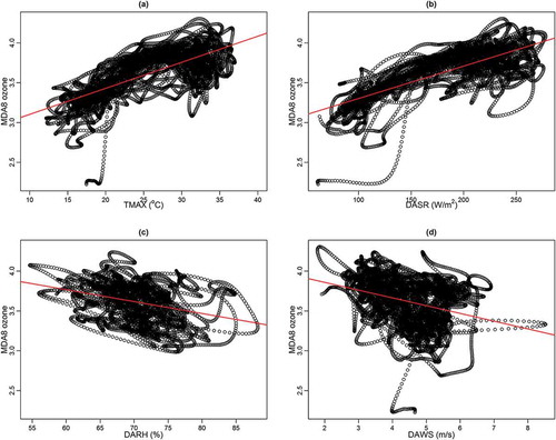
Linear regression analysis was conducted between the original, baseline (KZ_15,5), and short-term components of ozone and various combinations of meteorological variables, as per eqs 9, 10 and 12, 13. The results for the coefficient of determination (R²) are presented in Table 2 The selection of control variable combinations was based on a preliminary assessment of multiple collinearity among various meteorological variables, with detailed data for Pearson’s correlation coefficients provided in the supplementary information. The models in Table 2 were selected in order to limit variance inflation due to collinearity and provide interpretation of the physical phenomenon. The marked improvement in correlation achieved by the KZ filtering is evident in all baseline cases in comparisons with raw data. All the control variables combined could only explain 43.1% of the variability in raw ozone time series, whereas after the KZ filtering the cumulative effect of meteorological parameters could explain 61% of the variability in baseline ozone data. Solar radiation exhibits the strongest influence (R² = 0.585), with baseline ozone compared with temperature (R² = 0.487) qualitatively similar to the behavior observed for sites in the eastern United States (Milanchus, Trivikrama Rao, and Zurbenko 1998; Porter et al. 2001; Trivikrama, Zalewsky, and Zurbenko 1995; Wolff et al. 2001). Baseline ozone has weak negative correlations with relative humidity and resultant wind speed, as shown in Figure 5. Although DARH can be considered an important influence on raw ozone data (R² = 0.192), KZ_15.5 filtering reduced the strength of the correlation. This could be an anomaly resulting from the relatively narrow range of DARH values at the selected site (2000–2016). The influence of resultant wind speed alone is negligible even after filtering (R² = 0.099) and only slightly enhances the correlation in combination with other variables such as solar radiation (Model 5; R² = 0.591). The relatively lower R² values for linear relationship between baseline components of ozone and meteorological variables at this site are in contrast to ozone studies published for New York and Washington, DC, but closely match southwestern cities such as Phoenix and Tucson, indicating the relative importance of including location-specific mixing height data in future studies (Trivikrama and Zurbenko 1994; Trivikrama, Zalewsky, and Zurbenko 1995; Milanchus, Trivikrama Rao, and Zurbenko 1998; Wise and Comrie 2005a, 2005b).

Table 2. Coefficients of determination (R²) for linear regressions between raw data, baseline, and short-term components of MDA8 ozone and meteorological factors.

Parameter	Raw data	Baseline	Short-term
Model 1 (TMAX)	0.178	0.487	0.044
Model 2 (DASR)	0.390	0.585	0.286
Model 3 (DARH)	0.192	0.104	0.216
Model 4 (DAWS)	0.075	0.099	0.061
Model 5 (TMAX/DARH)	0.351	0.514	0.290
Model 6 (DASR/DAWS)	0.404	0.591	0.303
Model 7 (TMAX/DASR/DARH/DMWS)	0.431	0.614	0.372

Figure 5. Regression plots of baseline values of MDA8 ozone and (a) TMAX, (b) DASR, (c) DARH, and (d) DAWS.

Meteorological adjustment

Meteorologically adjusted MDA8 ozone residuals were computed as per eqs 11 and 14, and long-term trends of these residuals were calculated by the application of KZ_365,3 as per eq 15. This process was repeated for each model, and the residuals corresponding to each model (ε₁(t) to ε₇(t)) along with their correlations with meteorological variables are presented in the supplementary information. As the constructed long-term series were based on regression residuals and not real MDA8 ozone values in ppb, eq 17 was used to develop long-term components of meteorologically independent MDA8 ozone, and results for meteorologically adjusted time series are presented in Figure 6. The linear trends for these long-term time series were developed by fitting a time-controlled linear regression through the data in Figure 6, and the results are presented in Table 3. Data presented in Figure 6 also allow for a comparison of the meteorologically adjusted trends with the unadjusted long-term MDA8 component, e(t). For meteorological control variables that are positively correlated with ozone (TMAX and DASR), the model-adjusted trend line would be higher than the unadjusted trend line if the control variables are below their long-term averages, and vice versa. This effect is observed for most of the time period between the years 1997 and 2010 for Model 2 (DASR), the strongest control variable. During this period when control variables are below their long-term averages, any peaks in model-adjusted trend lines correspond to sudden increases in precursor emissions. For the time periods 1990–1996 and 2010–2014, the model-adjusted trend line is below the unadjusted trend line, indicating that during these periods solar radiation is higher than the long-term average DASR. For control variables that are negatively correlated with ozone (DARH and DAWS), model-adjusted trends are higher than unadjusted trends when the control variables are above their respective long-term averages. For the time period from 1990 to 1999, there is a positive trend in meteorologically independent MDA8 ozone, increasing at an average linear rate of 0.292 ± 0.022 ppb/yr. These results for the 2000–2016 period suggest a negative linear trend as high as −0.547 ± 0.009 ppb/yr and as low as −0.320 ± 0.005 ppb/yr. When the effects of all meteorological variables are removed, MDA8 ozone at the current site decreases at a rate of 0.412 ± 0.007 ppb/yr, indicating the moderate success of emission control programs in the HGB area post 2000. These trend results are comparable to research reported by Souri et al. (2016), which estimated that overall MDA8 ozone concentrations for continuous ambient monitoring stations (CAMS) network in Houston decreased at a rate of 0.6 ± 0.3 ppb/yr for the time period 2000–2014. This decline reported by Souri et al. (2016) can be attributed to a combined influence of emissions and meteorology; Souri et al. further examined the effect of long-term wind patterns on ozone in Houston (Souri et al. 2016). Asitha et al. (2017) conducted a dynamic evaluation of the fully coupled Weather Research and Forecasting (WRF)–Community Multiscale Air Quality (CMAQ) model simulations for summer (May–September) ozone over the period 1990–2010 and reported linear trends for various regions of the United States (Astitha et al. 2017). For the South-Central region, which includes the HGB area, a positive trend of 0.79 ppb/yr and a negative trend of 1.18 ppb/yr were simulated for the years 1990–2000 and 2000–2010, respectively. This study also compared the simulated trends with observed summertime trends for 21 AQS sites in the South-Central region, decreasing at an average rate of 1.40 ppb/yr for the years 2000–2010. The results presented in the current study for the Aldine site are in agreement with the overall trends observed by Astitha et al. (2017) and with the downward trend (0.52 ± 0.18 ppb/yr) in summertime ozone mixing ratios for the years 2005–2013 for Houston reported by Choi and Souri (2015), Astitha et al. (2017, and Choi and Souri (2015).

Table 3. Estimated linear trends for long-term meteorologically independent MDA8 ozone (ppb/yr) at Aldine.

Model	Linear trend 1990–2016 (ppb/yr)	Linear trend 1990–1999 (ppb/yr)	Linear trend 2000–2016 (ppb/yr)
Model 1 (TMAX)	−0.118 ± 0.004 (R^2 = 0.245, P < 0.05)	0.258 ± 0.017 (R^2 = 0.198, P < 0.05)	−0.320 ± 0.005 (R^2 = 0.716, P < 0.05)
Model 2 (DASR)	−0.140 ± 0.005 (R^2 = 0.218, P < 0.05)	0.292 ± 0.023 (R^2 = 0.141, P < 0.05)	−0.334 ± 0.008 (R^2 = 0.531, P < 0.05)
Model 3 (DARH)	—*	—*	−0.547 ± 0.009 (R^2 = 0.663, P < 0.05)
Model 4 (DAWS)	−0.145 ± 0.005 (R^2 = 0.246, P < 0.05)	0.250 ± 0.014 (R^2 = 0.101, P < 0.05)	−0.256 ± 0.008 (R^2 = 0.396, P < 0.05)
Model 5 (TMAX/DARH)	—	—*	−0.517 ± 0.005 (R^2 = 0.837, P < 0.05)
Model 6 (DASR/DAWS)	−0.155 ± 0.005 (R^2 = 0.268, P < 0.05)	0.292 ± 0.022 (R^2 = 0.160, P < 0.05)	−0.372 ± 0.007 (R^2 = 0.634, P < 0.05)
Model 7 (TMAX/DASR/DARH/DMWS)	—*	—*	−0.412 ± 0.007 (R^2 = 0.634, P < 0.05)

Note.*Data not available for relative humidity during the years 1990–1999.

Figure 6. Long-term components of meteorologically independent MDA8 ozone concentrations (ppb) at Aldine. (a) single-regression models; (b) multiple-regression models.

Exploration of possible causes for decreasing meteorologically independent ozone was carried out by developing long-term components for time series of the NO_x (NO, NO₂) and NO_y data. From Figure 7, it is evident that the major continuous drop in NO₂ emissions starts after 2000 (50% decrease in 16 yr), whereas NO concentration drastically reduces in two phases: an initial decrease of 50% from 1990 to 1996 and another 50% decrease between 1998 and 2009. Even though there seems to be a 40% decrease in the NO_y long-term component from 2004 to 2008, due to limited data availability NO_y cannot be interpreted to be responsible for negative MDA8 ozone trends. A linear regression analysis between the long-term components of NO, NO₂, NO_x, NO_y, and meteorologically independent MDA8 ozone was conducted to establish quantitative factors for comparison. From the R² values in Table 4, it is evident that NO, NO₂, and NO_x are the major factors controlling the negative trend of MDA8 ozone at this location. The effect of NO is stronger for Models 3, 5 and 7, when data post 2000 are considered due to the absence of DARH data until 1999, whereas NO₂ exerts stronger control when the overall 27-yr data are considered. In Models 1, 2 and 6, where the complete data set from 1990 to 2016 is included, emission reductions in NO_x could explain an average of 34% of the long-term variability in MDA8 ozone data. However, with the data set limited to 2000–2016 and all four meteorological variables included in the model, 64% of the long-term variability in meteorologically adjusted MDA8 ozone could be attributed to NO_x emissions. The contribution of NO_y emissions toward lowering of meteorologically adjusted MDA8 ozone could be around 25% post 2005. Yearly statistics of daily maximum HRVOC concentrations (ppb of carbon) from 1997 to 2013 at the Aldine site were calculated and are presented as a box plot in Figure 8. The highest yearly maximum HRVOC concentration of 86.7 ppb of carbon was observed for the year 2000, and the lowest yearly maximum (24.2 ppb of carbon) was observed in 2011. An overall linear rate of decrease was calculated to be 3.52 ± 1.19 ppb/yr (R² = 0.727, P < 0.05) over the 17 yr. This reduction in HRVOC levels is consistent with the 20–50% decline in radical (HO_x and RO_x) production observed between the Texas Air Quality Studies of 2000 and 2006 (Zhou, Cohan, and Henderson 2014). Additionally, the ratio of 1-hr daily maximum ozone (MDA1) to MDA8 at the Aldine site was calculated, and the KZ filter was applied to the ratio of MDA1/MDA8. Since MDA1 values are more sensitive to HRVOC emissions, a significant downward trend in the long-term component of MDA1/MDA8 lends further evidence to the success of HRVOC emission controls post 2003. This result, presented in Figure 9, indicates a negative trend for the long-term component of the ratio, from a high of 1.4 in 1994 to a low of 1.2 in 2014. This reduction in HRVOC emissions at Aldine could be attributed due to the HGB area ozone attainment SIP in December 2002, which targeted HRVOC emissions from fugitives, flares, process vents, and cooling towers (TCEQ 2017b, 2017c). Between the years 2003 and 2013, a 43% reduction in the yearly maximum of HRVOC concentrations could be observed at this site, which could have played a significant role complimenting the lower NO_x levels. The overall reduction in emissions of ozone precursors contributed to decrease in meteorologically independent MDA8 ozone at this site. The trends presented in this study could enable future research on the effectiveness of further NO_x and HRVOC emission control strategies for air quality management in the HGB area.

Table 4. Coefficients of determination (R²) for linear regressions between long-term meteorologically adjusted MDA8 and long-term components of nitrogen oxides.

Parameter	eNO2(t)	eNO(t)	eNOx(t)	eNOy(t)
Model 1 (TMAX)	0.359	0.199	0.360	0.311
Model 2 (DASR)	0.286	0.234	0.306	0.246
Model 3 (DARH)	0.591	0.738	0.738	0.174
Model 4 (DAWS)	0.181	0.229	0.243	0.092
Model 5 (TMAX/DARH)	0.741	0.837	0.846	0.340
Model 6 (DASR/DAWS)	0.333	0.257	0.350	0.295
Model 7 (TMAX/DASR/DARH/DMWS)	0.595	0.612	0.638	0.252

Figure 7. Long-term components of nitrogen oxides at Aldine in the HGB area. (a) NO₂ and NO; (b) NO_X and NO_y.

Figure 8. Box plot with yearly statistics for daily maximum HRVOC concentrations at Aldine, during 1997–2013. Open squares represent means; dots represent maximum values; line dividing the boxes represents the median; upper and lower limits of boxes represent third and first quartiles; and whisker length represents 1.5 times interquartile distance.

Figure 9. Decomposed time series of the ratio of MDA1/MDA8 ozone at Aldine, during 1990–2016. (a) original ratio; (b) long-term trend component; (c) seasonal component; (d) short-term component.

Conclusion

In the current study, the KZ filter method was applied to MDA8 ozone data from 1990 to 2016 at an urban site (EPA AQS Site ID: 48-201-0024) located within 10 miles of downtown Houston and the George Bush Intercontinental Airport. The MDA8 ozone time series was separated into long-term, seasonal, and short-term components in order to facilitate the meteorological adjustment with four single-regression (temperature, solar radiation, relative humidity and resultant wind speed) and three multiple-regression models. The short-term component of ozone could explain 63% of the total variance observed in MDA8 ozone time series, indicating a strong effect of mesoscale day-to-day variability at this location. This process allowed for a comprehension of relative contributions of meteorological control variables toward variance in ozone time series and enabled us to develop linear regressions between various combinations of meteorological variables and ozone. We found that solar radiation exhibits the strongest correlation with baseline ozone (R² = 0.585) at this site, compared with temperature (R² = 0.487). The regression model including all four meteorological variables (temperature, solar radiation, relative humidity, wind speed) explains 61% of the variance in baseline MDA8 ozone. Long-term trends for MDA8 ozone, independent of the influence of meteorological factors, were constructed for 1990–2016, and the overall linear trends were calculated to be in the range of −0.118 ± 0.004 to −0.155 ± 0.005 ppb/yr. A greater rate of decrease was observed for data between 2000 and 2016 (−0.320 ± 0.005 to −0.547 ± 0.009 ppb/yr), whereas the data from 1990 to 1999 show increasing trends in isolation. Long-term meteorologically independent MDA8 data reveal a high degree of correlation with oxides of nitrogen (NO_x and NO_y) data in general and NO_x in particular. Long-term trend components of NO and NO₂ could explain 61.2% and 59.5% of the variability in trends observed for MDA8 ozone post 2000. The daily maximum HRVOC concentrations decreased by 43% between 2003 and 2013 at Aldine, complimenting the reduction in NO_x levels and the two being cumulatively responsible for the decrease in MDA8 trends reported in the current study. This result indicates the success of NO_x and HRVOC emission control policies in the HGB area positively affecting ozone air quality at this site. However, future research on the application of the KZ filter method to multiple sites distributed across the HGB area could facilitate a broader and more comprehensive evaluation of the effectiveness of air quality management in the Texas gulf coast. A great need also exists in expanding the KZ filter method with other meteorological parameters such as mixing heights and wind patterns.

Supplemental data

Supplemental data for this paper can be accessed on the publisher’s website.

Additional information

Funding

This research is supported by the National Science Foundation (NSF) through the Center for Energy & Environmental Sustainability (CEES), an NSF CREST Center (award no. 1036593). The technical content of this paper is solely the responsibility of the authors.

Notes on contributors

Venkata S.V. Botlaguduru

Venkata S.V. Botlaguduru is a postdoctoral researcher at the Center for Energy & Environmental Sustainability, Prairie View A&M University, Prairie View, TX.

Raghava R. Kommalapati

Raghava R. Kommalapati is a professor in the Department of Civil & Environmental Engineering and the director of the Center for Energy & Environmental Sustainability, Prairie View A&M University, Prairie View, TX.

Ziaul Huque

Ziaul Huque is a professor in the Department of Mechanical Engineering and a senior researcher at Center for Energy & Environmental Sustainability, Prairie View A&M University, Prairie View, TX.

References

- Astitha, M., S. Huiying Luo, T. Rao, C. Hogrefe, R. Mathur, and N. Kumar. 2017. Dynamic evaluation of two decades of WRF-CMAQ ozone simulations over the contiguous United States. Atmos. Environ. 164:102–116. doi:10.1016/j.atmosenv.2017.05.020.
- Banta, R.M., C.J. Senff, J. Nielsen-Gammon, L.S. Darby, T.B. Ryerson, R.J. Alvarez, S.P. Sandberg, E.J. Williams, and M. Trainer. 2005. A bad air day in Houston. Bull. Am. Meteorol. Soc. 86 (5):657–669. doi:10.1175/bams-86-5-657.
- Berlin, S.R., A.O. Langford, M. Estes, M. Dong, and D.D. Parrish. 2013. Magnitude, decadal changes, and impact of regional background ozone transported into the greater Houston, Texas, area. Environ. Sci. Technol. 47 (24):13985–13992. doi:10.1021/es4037644.
- Brown, S.S., W.P. Dubé, R. Bahreini, A.M. Middlebrook, C.A. Brock, C. Warneke, J.A. de Gouw, R.A. Washenfelder, E. Atlas, J. Peischl, T.B. Ryerson, J.S. Holloway, J.P. Schwarz, R. Spackman, M. Trainer, D.D. Parrish, F.C. Fehshenfeld, and A.R. Ravishankara. 2013. Biogenic voc oxidation and organic aerosol formation in an urban nocturnal boundary layer: aircraft vertical profiles in houston, tx. Atmos. Chem. Phys. 13 (22):11317-11337. doi: 10.5194/acp-13-11317-2013.
- Choi, Y., and A.H. Souri. 2015. Chemical condition and surface ozone in large cities of Texas during the last decade: Observational evidence from OMI, CAMS, and model analysis. Remote. Sens. Environ. 168:90–101. doi:10.1016/j.rse.2015.06.026.
- Eskridge, R.E., J. Yeong, S. Ku, P. Trivikrama Rao, S. Porter, and I.G. Zurbenko. 1997. Separating different scales of motion in time series of meteorological variables. Bull. Am. Meteorol. Soc. 78 (7):1473–1483. doi:10.1175/1520-0477(1997)078<1473:sdsomi>2.0.co;2.
- Gardner, M.W., and S.R. Dorling. 2000. Meteorologically adjusted trends in UK daily maximum surface ozone concentrations. Atmos. Environ. 34 (2):171–176. doi:10.1016/S1352-2310(99)00315-5.
- Hogrefe, C.S., T. Rao, I.G. Zurbenko, and P.S. Porter. 2000. Interpreting the information in ozone observations and model predictions relevant to regulatory policies in the eastern United States. Bull. Am. Meteorol. Soc. 81 (9):2083–2106. doi:10.1175/1520-0477(2000)081<2083:itiioo>2.3.co;2.
- Ibarra-Berastegi, G., I. Madariaga, A. Elı́as, E. Agirre, and J. Uria. 2001. Long-term changes of ozone and traffic in Bilbao. Atmos. Environ. 35 (32):5581–5592. doi:10.1016/S1352-2310(01)00210-2.
- Kang, D., C. Hogrefe, K.L. Foley, S.L. Napelenok, R. Mathur, and S. Trivikrama Rao. 2013. Application of the Kolmogorov-Zurbenko filter and the decoupled direct 3D method for the dynamic evaluation of a regional air quality model. Atmos. Environ. 80:58–69. doi:10.1016/j.atmosenv.2013.04.046.
- Kleinman, L.I., P.H. Daum, D. Imre, Y.-N. Lee, L.J. Nunnermacker, S.R. Springston, J. Weinstein-Lloyd, and J. Rudolph. 2002. Ozone production rate and hydrocarbon reactivity in 5 urban areas: a cause of high ozone concentration in houston. Geophys. Res. Lett. 29:10. doi: 10.1029/2001GL014569.
- Maxwell-Meier, K.L., and M.E. Chang. 2005. Comparison of ozone temporal scales for large urban, small urban, and rural areas in Georgia. J. Air Waste Manage. Assoc. 55 (10):1498–1507. doi:10.1080/10473289.2005.10464750.
- Milanchus, M.L., S. Trivikrama Rao, and I.G. Zurbenko. 1998. Evaluating the effectiveness of ozone management efforts in the presence of meteorological variability. J. Air Waste Manag. Assoc. 48 (3):201–215. doi:10.1080/10473289.1998.10463673.
- Morris, G.A., B. Ford, A.M. Bernhard Rappenglück, A.M. Thompson, F. Ngan, and B. Lefer. 2010. An evaluation of the interaction of morning residual layer and afternoon mixed layer ozone in Houston using Ozone Sonde data. Atmos. Environ. 44 (33):4024–4034. doi:10.1016/j.atmosenv.2009.06.057.
- National Renewable Energy Laboratory. 2017. National Solar Radiation Database. Accessed March, 2017. http://rredc.nrel.gov/solar/old_data/nsrdb/1991-2010/hourly/siteonthefly.cgi?id=722430.
- Parrish, D.D., D.T. Allen, T.S. Bates, M. Estes, F.C. Fehsenfeld, G. Feingold, R. Ferrare, R.M. Hardesty, J.F. Meagher, J.W. Nielsen-Gammon, R.B. Pierce, T.B. Ryerson, J.H. Seinfeld, and E.J. Williams. 2009. Overview of the second Texas Air Quality Study (TexAQS II) and the Gulf of Mexico Atmospheric Composition and Climate Study (GoMACCS). J. Geophys. Res. Atmos. 114 (D7):n/a-n/a. doi:10.1029/2009JD011842.
- Rao, S.T., I.G. Zurbenko, R. Neagu, P.S. Porter, J.Y. Ku, and R.F. Henry. 1997. Space and time scales in ambient ozone data. Bull. Am. Meteorol. Soc. 78 (10):2153–2166. doi:10.1175/1520-0477(1997)078<2153:satsia>2.0.co;2.
- Sá, E., O. Tchepel, A. Carvalho, and C. Borrego. 2015. Meteorological driven changes on air quality over Portugal: A KZ filter application. Atmos. Pollut. Res. 6 (6):979–989. doi:10.1016/j.apr.2015.05.003.
- Souri, A.H., Y. Choi, L. Xiangshang, A. Kotsakis, and X. Jiang. 2016. A 15-year climatology of wind pattern impacts on surface ozone in Houston, Texas. Atmos. Res. 174 (Suppl. C):124–134. doi:10.1016/j.atmosres.2016.02.007.
- Steven, P.P., S. Trivikrama Rao, I.G. Zurbenko, A.M. Dunker, and G.T. Wolff. 2001. Ozone air quality over North America: Part II—An analysis of trend detection and attribution techniques. J. Air Waste Manage. Assoc. 51 (2):283–306. doi:10.1080/10473289.2001.10464261.
- Texas Commission on Environmental Quality. 2017a. Houston-Galveston-Brazoria: Ozone history. Accessed July, 2017. https://www.tceq.texas.gov/airquality/sip/hgb/hgb-ozone-history.
- Texas Commission on Environmental Quality. 2017b. Texas SIP Revisions. Accessed July, 2017. https://www.tceq.texas.gov/airquality/sip/sipplans.html.
- Texas Commission on Environmental Quality. 2017c. History of the Texas State Implementation Plan (SIP). Accessed July, 2017. https://www.tceq.texas.gov/airquality/sip/sipintro.html#what-is-the-history.
- Trivikrama, R.S., E. Zalewsky, and I.G. Zurbenko. 1995. Determining temporal and spatial variations in ozone air quality. J. Air Waste Manage. Assoc. 45 (1):57–61. doi:10.1080/10473289.1995.10467342.
- Trivikrama, R.S., and I.G. Zurbenko. 1994. Detecting and tracking changes in ozone air quality. Air Waste 44 (9):1089–1092. doi:10.1080/10473289.1994.10467303.
- U.S. Census Bureau. 2016. QuickFacts: Houston City, Texas. U.S. Census Bureau Web site. Accessed June, 2017.https://www.census.gov/quickfacts/fact/table/houstoncitytexas/PST045216.
- U.S. Environmental Protection Agency. 2016. Our nation’s air: Status and trends through 2016. Accessed September, 2017.https://gispub.epa.gov/air/trendsreport/2017/#home.
- U.S. Environmental Protection Agency. 2017a. Nonattainment areas for criteria pollutants (Green Book). Accessed August, 2017. https://www3.epa.gov/airquality/greenbook/hbtc.html.
- U.S. Environmental Protection Agency. 2017b. Air data: Air quality data collected at outdoor monitors across the US. Accessed March, 2017. https://www.epa.gov/outdoor-air-quality-data.
- U.S. Environmental Protection Agency. 2018. Air quality design values: Ozone design values, 2016. Accessed February, 2017. https://www.epa.gov/air-trends/air-quality-design-values.
- U.S. Environmental Protection Agency. 2011. The benefits and costs of the Clean Air Act from 1990 to 2020. Washington, DC: U.S. Environmental Protection Agency.
- Washenfelder, R.A., M. Trainer, G.J. Frost, T.B. Ryerson, E.L. Atlas, J.A. De Gouw, F.M. Flocke, A. Fried, J.S. Holloway, D.D. Parrish, J. Peischl, D. Richter, S.M. Schauffler, J.G. Walega, C. Warneke, P. Weibring, and W. Zheng. 2010. Characterization of NOx, SO2, ethene, and propene from industrial emission sources in Houston, Texas. J. Geophys. Res. Atmos. 115 (D16):n/a-n/a. doi:10.1029/2009JD013645.
- Wise, E.K., and A.C. Comrie. 2005a. Extending the Kolmogorov–Zurbenko Filter: Application to ozone, particulate matter, and meteorological trends. J. Air Waste Manage. Assoc. 55 (8):1208–1216. doi:10.1080/10473289.2005.10464718.
- Wise, E.K., and A.C. Comrie. 2005b. Meteorologically adjusted urban air quality trends in the southwestern United States. Atmos. Environ. 39 (16):2969–2980. doi:10.1016/j.atmosenv.2005.01.024.
- Wolff, G.T., A.M. Dunker, S. Trivikrama Rao, P. Steven Porter, and I.G. Zurbenko. 2001. Ozone air quality over North America: Part I—A review of reported trends. J. Air Waste Manage. Assoc. 51 (2):273–282. doi:10.1080/10473289.2001.10464270.
- Yang, W., and I. Zurbenko. 2010. Kolmogorov–Zurbenko filters. Wiley Interdiscip. Rev. Comput. Stat. 2 (3):340–351. doi:10.1002/wics.71.
- Zhou, W., D.S. Cohan, and B.H. Henderson. 2014. Slower ozone production in Houston, Texas following emission reductions: Evidence from Texas air quality studies in 2000 and 2006. Atmos. Chem. Phys. 14 (6):2777–88. doi:10.5194/acp-14-2777-2014.