Comparing emission rates derived from a model with those estimated using a plume-based approach and quantifying the contribution of vehicle classes to on-road emissions and air quality

ABSTRACT

This study presents a comparison of fleet average emission factor (s) derived from a traffic emission model with EFs estimated using plume-based measurements, including an investigation of the contribution of vehicle classes to carbon monoxide (CO), nitrogen oxides (NO_x), and elemental carbon (EC) along an urban corridor. To this end, a field campaign was conducted over one week in June 2016 on an arterial road in Toronto, Canada. Traffic data were collected using a traffic camera and a radar, whereas air quality was characterized using two monitoring stations: one located at ground level and another at the rooftop of a four-story building. A traffic simulation model was calibrated and validated, and second-by-second speed profiles for all vehicle trajectories were extracted to model emissions. In addition, dispersion modeling was conducted to identify the extent to which differences in emissions translate to differences in near-road concentrations. The results indicate that modeled EFs for CO and NO_x are twice as high as plume-based EFs. Besides, modeled results indicate that transit bus emissions accounted for 60% and 70% of the total emissions of NO_x and EC, respectively. Transit bus emission rates in g/passenger·km for NO_x and EC were up to 8 and 22 times, respectively, the emission rates of passenger cars. In contrast, the Toronto streetcars, which are electrically fueled, were found to improve near-road air quality despite their negative impact on traffic speeds. Finally, we observe that the difference in estimated concentrations derived from the two methods is not as large as the difference in estimated emissions due to the influence of meteorology and of the urban background given that the study network is located in a busy downtown area.

Implications: This study presents a comparison of fleet average emission factor (s) derived from a traffic emission model with EFs estimated using plume-based measurements, including an investigation of the contribution of vehicle classes to various pollutants. Besides, dispersion modeling was conducted to identify the extent to which differences in emissions translate to differences in near-road concentrations. It was observed that the difference in estimated concentrations derived from the two methods is not as large as the difference in estimated emissions due to the influence of meteorology and of the urban background, as the study network is located in a busy downtown area.

Introduction

Through a combination of regulation and improved technology, tailpipe emissions from light-duty vehicles have declined substantially over the past several decades. Important milestones included the introduction of fuel injection, positive crankcase ventilation, exhaust gas recirculation, catalytic converters, and on-board diagnostic systems. However, despite these reductions and the large improvements in urban air quality, epidemiological evidence continues to reveal significant associations between traffic-related air pollution (TRAP) and health (Fuertes et al. 2013).

The challenge of reducing TRAP remains ever present (and increasingly complex) due to the emergence of new trends facing urban transportation systems, such as the increasing popularity of gasoline direct injection (GDI) vehicles (Zhao, Stone, and Zhou 2010). Recent research on GDI engines demonstrated high fuel efficiency at the expense of increased emissions of black carbon (or soot) and toxic substances (Zimmerman et al. 2016). Moreover, the complexity of individual mobility needs and the rise of sharing economies (on-demand transit, ride-sharing, autonomous vehicles) will affect the spatiotemporal distribution of emissions and introduce new vehicle types into the fleet. Finally, the rise in urban freight movements will replace some passenger trips but increase the proportion of small and medium trucks on the road.

In order to anticipate the effects of these trends on air quality and health and inform the development of policies and standards governing vehicles and fuels, accurate emission inventories are essential. Efforts in integrating traffic models with emission models for the purpose of generating emission inventories or for evaluating traffic-related air pollution are in constant evolution. The scale of emission simulation ranges from a single road, to regional networks, and further to state and national inventories (Thunis et al. 2016). Furthermore, different types of dispersion models have been used to quantify the concentrations of air pollutants in near-road environments, and estimate personal exposures, such as Gaussian dispersion models and street-canyon models (Soulhac et al. 2011).

The accuracy of emission inventories or near-road air pollution concentrations mostly rely on the accuracy of the emission estimates, which depend on the quality of the emission factors (EFs). To date, various methods have been used to estimate EFs. The emission profiles of vehicles can be measured under real-world conditions, such as through remote sensing and tunnel studies. An analysis of remote sensing data across the United Kingdom indicated that roughly half the total nitrogen oxide (NO_x) emissions in an urban road were due to heavy-duty vehicles (HDVs) and buses (Carslaw et al. 2011). In Sao Paulo, measurements conducted in two tunnels revealed that fleet averaged EFs were heavily influenced by the fraction of HDVs, as the EFs for HDVs were 3.6 ± 1.5 and 9.2 ± 2.7 g/veh·km, for carbon monoxide (CO) and NO_x (Pérez-Martínez et al. 2014). In another study, elemental carbon (EC) with an EF of 131 ± 14 mg/veh·km was found to be the most abundant portion of PM_2.5 (particulate matter with an aerodynamic diameter ≤2.5 μm) from on-road diesel-fueled vehicles estimated in a tunnel in Hong Kong (Cheng et al. 2010).

Other real-world EFs measurements have been conducted on mobile platforms. A recent field study in Beijing used a mobile fast response instrument for conducting on-road chasing studies and found that 20% of diesel trucks were responsible for 50% of total CO emissions and over 70% of EC emissions (Wang et al. 2011b). In addition, the chasing method was used in Slovenia to emphasize a disproportionate contribution of high emitters to the fleet’s total emissions: the top 25% of diesel vehicles produced 63, 47, and 61% of EC, NO_x, and particle number emissions, respectively (Ježek et al. 2015). A portable emission measurement system (PEMS) was used in on-board measurements in Beijing and determined bus EFs for CO and NO_x, to be in the range of 1.3–12.7 and 3.0–12.8 g/veh·km, respectively (Wang et al. 2011a). A study in Italy used PEMS to analyze on-road emissions and found that NO_x emissions of diesel vehicles were 0.93 ± 0.39 g/veh·km (Weiss et al. 2011).

In the United States, where emission inventories are conducted at the metropolitan, state, and national levels, much of the work is conducted using the U.S. Environmental Protection Agency (EPA) model MOVES (MOtor Vehicle Emissions Simulator). The MOVES model, which is also adopted in Canada, is based on emission data from inspection and maintenance programs and dynamometer tests in various U.S. cities, including but not limited to Chicago, Phoenix, New York, Maryland (EPA 2015a, 2015b). These data are based on test cycles that are limited in terms of the range of speed and tractive power that they cover. In fact, findings from recent studies suggest that NO_x emissions are overestimated in the MOVES model. These studies performed chemical transport modeling and found that better agreement with ambient monitoring data, satellite observations, and/or aircraft measurements could be achieved by reducing NO_x emissions by 50–100% (Bai et al. 2016). Few studies have compared MOVES results with PEMS data. The most noteworthy is a recent comparison with PEMS conducted by Liu et al. (Liu and Frey 2015), who tested approximately 100 light-duty gasoline vehicles in North Carolina and found that the MOVES-modeled emission rates were up to 3 times higher than measured rates. This vehicle sample did not capture high emitters and cold starts, which can account for part of the disagreement.

In the Canadian context, there are no emission models currently endorsed by Environment Canada; therefore, the MOVES model is often used with default U.S. nationwide data. Although similarities between new vehicles sold in Canada and the United States are present, the differences in driving and meteorological conditions will lead to different deterioration rates of the in-use vehicle fleet. There is a need for comparing MOVES predictions with independent data and assess whether trends in bias appear across multiple sources.

This study aims to compare emission estimates generated from the emission model MOVES with detailed local inputs and plume-based measurements of fleet averaged EFs for vehicles running along a busy road in Toronto, Canada. The plume-based analysis could only generate fleet averaged EFs that could be dominated by high emitters. As such, modeling was further employed to examine the contributions of different vehicle classes and shed light on the differences between the two methods. Finally, EFs derived from MOVES and plume measurements were used as input in a street-canyon dispersion model to capture the effects of difference in EFs on the resulting estimates of near-road air quality.

Materials and methods

Study area and data collection sites

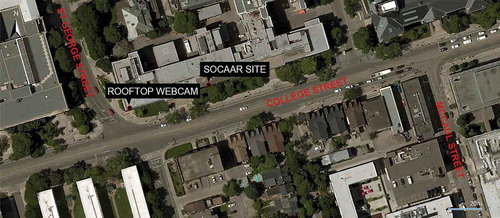
Our study area includes a single road segment on College Street, a four-lane arterial road in downtown Toronto, Canada. The study segment is located between two major signalized intersections: College Street and Saint George Street on the west, as well as College Street and McCaul Street on the east. Along the segment are multiple-story buildings on both sides of the road: University of Toronto buildings on the north side and a mix of commercial and residential buildings on the south side, representing a typical urban canyon environment.

Typically, electric-powered streetcars (light rail) run in the middle lanes of College Street offering public transportation service. However, during the week we selected for data collection (June 17–24, 2016), streetcars were substituted by diesel-fueled transit buses running along College Street without dedicated lanes. This offered a unique possibility to study the effect of transit buses on total emissions as well as compare the effect of transit buses with the effect of streetcars.

Traffic and air quality data collection occurred over a week in the month of June 2016 (June 17–24) at two sites: (1) rooftop level: on the rooftop of a four-story University of Toronto building at the intersection between College Street and Saint George Street, where traffic, meteorology, and air pollution data were collected; (2) street level: at the Southern Ontario Center for Atmospheric Aerosol Research (SOCAAR) located on the north side, where traffic data were recorded by a webcam as well as detected by a microwave radar system (SmartSensor HD; Wavetronix, Provo, UT, USA). At the same point, ambient air was drawn through inlets located 15 m from the roadway and 3 m aboveground. All data in this study were provided by SOCAAR. Figure 1 presents our study area and two data collection sites.

Figure 1. Study area and data collection sites.

Generation of modeled emissions

The modeled EFs for CO, NO_x, and EC were developed using an integrated modeling approach, which involves a traffic microsimulation model and a microscopic emission model. The traffic microsimulation model was calibrated based on traffic data extracted from raw footage of vehicles at the intersection, then the simulated driving behaviors along the study corridor were processed to provide inputs to the emission model, which generated distance-based EFs (in g km⁻¹) for various pollutants based on the vehicle types.

Traffic simulation

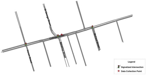
In this study, a microscopic traffic simulation model was developed for the study area using the PTV Vissim platform (Vissim 9.0; PTV, Karlsruhe, Germany). As shown in Figure 2, the simulated network was expanded to include two additional signalized intersections upstream and downstream of the intersection between College Street and Saint George Street, in order to capture driving behaviors at the intersection, such as acceleration, deceleration, and queuing. The road configuration was gathered based on Google maps and confirmed through field visits. The width of each lane was set as 3.3 m; roadway gradients were assigned as 0%.

Figure 2. The traffic simulation network (using the PTV Vissim platform).

Traffic information, including vehicle volumes, vehicle types, and their corresponding routing decisions, was manually derived from the recorded video images at the intersection. Vehicles were noted as passenger cars, passenger trucks, transit buses, intercity buses, school buses, refuse trucks, single-unit short-haul trucks (or medium trucks), and single-unit long-haul trucks (or large trucks). Traffic signal timings and turning restrictions were obtained through field visits. Besides, the public transport routes were included in the network by locating transit bus stops on the two sides of the road. The dwell time distribution was defined by estimating the distribution of time difference for each transit bus passing through two webcams at street level and rooftop level. For each simulation run, a 900-sec warm-up time was used to load vehicles onto the network.

A data collection point was located in the simulation network at the same place where the radar is positioned on the study segment. Two types of outputs were derived from the microsimulation model: (1) vehicle records at the data collection point, including vehicle counts, vehicle types, and instantaneous speeds; and (2) second-by-second trajectories of each vehicle from the moment it enters the network until it exits the network. The traffic simulation model was first validated against the radar records in terms of the vehicle counts and then calibrated using a number of parameters to improve the model’s ability to replicate the real-world distribution of speeds as detected by the radar. Two hours (6 p.m.–8 p.m.) on Thursday were used for the calibration. The calibrated parameters were maintained for the rest of the simulation hours. Further information on the calibration of the traffic simulation model is provided in the supplement.

Emission modeling

The EPA MOVES model (MOVES2014a; EPA, Washington, D.C., U.S.) was adopted to estimate the emissions of different pollutants, including CO, NO_x, and EC, based on instantaneous speed data from the simulation model. The use of second-by-second speed profiles as the link activity enables the emission model to take into account detailed driving behaviors, including acceleration, deceleration, cruising, and idling, making the results more realistic compared with those of the aggregated method of using hourly average speeds for all vehicles on the link.

Besides link activity, MOVES needs information on link characteristics, vehicle types, model years, fuel information, and meteorology. The road type was set as “urban unrestricted road.” Vehicle types were obtained from the simulated traffic outputs. Vehicle model year data were derived from the Drive Clean program, the provincial inspection and maintenance program (Melorose, Perroy, and Careas 2015). Meteorological data were extracted from the local meteorology station on the rooftop of the University of Toronto building, including hourly temperature (°F) and relative humidity (%). Moreover, all passenger cars, passenger trucks, and light commercial trucks were assumed to run on gasoline, whereas other vehicles were assumed to run on diesel (Natural Resources Canada 2009). Only “running exhaust emissions” were estimated.

The fleet averaged EF was calculated as a weighted value based on the estimated emissions from different vehicle classes and the proportion of each vehicle type. Total emissions on the study segment were calculated by summing the estimated emissions of each vehicle passing through the link.

Comparing segment emissions, with transit bus versus streetcar service

To investigate the effect of public transit on segment emissions, another traffic data collection was conducted on two weekdays in the month of April 2016 (April 28 and 29). During this period, electric-powered streetcars ran along the dedicated middle lanes of College Street.

Traffic data were manually extracted from the webcams and were then employed as inputs for the traffic simulation model. Unlike the network with transit bus service, the streetcar stops were located in the middle lanes; vehicles need to wait behind the streetcars when they stop at the stations, to allow passengers to cross the road. Traffic simulation was also calibrated and validated by identifying the parameters and parameter values, which ensure that the influence of streetcars on traffic conditions was appropriately represented.

The selected parameters were then used to conduct the same simulation as the one with transit bus service on Thursday and Sunday in June 2016, and all traffic inputs were kept the same while transit stops were moved from two sides of the road to the central lanes representing street car service. The aim of this exercise is to compare segment emissions, with transit bus versus streetcar service, using the same traffic demand for the same time period.

Generation of plume-based emissions

Plume-based EFs were developed under real-world conditions using an automated identification and integration method to analyze exhaust plumes of passing vehicles based on high-time-resolution air pollution measurements (Wang et al. 2015). During the study period (June 17–24, 2016), various air pollutants, including CO and NO_x, were continuously measured.

Measurement technique

Ambient air at street level was drawn through inlets and distributed among various instruments. CO was measured using a gas filter correlation infrared analyzer, and NO_x was measured using a chemiluminescence analyzer (410i and 48C, respectively; Thermo Scientific, Waltham, MA, USA). The time resolution for CO measurements was 10 sec and for NO_x, 1 sec.

Simultaneously, local meteorology data, including temperature, humidity, as well as wind speed and direction, were measured by a meteorological station (WXT520; Vaisala, Vantaa, Finland), located at rooftop level. The passing vehicles were detected by a SmartSensor HD (SS-125; Wavetronix) dual-radar system, and vehicles were categorized as light-duty (1.5–7 m) or heavy-duty (7–18 m) vehicles based on the detected length.

Data analysis

All measured pollutants were time corrected to match with the carbon dioxide (CO₂) signal by conducting a sensitivity analysis that shifted the time series of each pollutant in 1-sec increments in order to find the most appropriate lag time. Then, an automated identification method was used to detect vehicle exhaust plumes based on the inflection points before and after a plume estimated from the slope of the CO₂ signal averaged over 10 sec (Wang et al. 2015). The plumes represented emissions generated from a certain number of vehicles passing through the data collection point.

Measured emissions were processed to develop fuel-based emission factors (EFs), which can be defined as grams of pollutant emitted for every kilogram of fuel burned. The EFs for various pollutants were estimated using CO₂ and CO as a measure of fuel burned (eq 1), given that the conversion efficiency of carbon in fuel to CO₂ is close to 99% when gasoline and diesel engines are under normal operation (Franco et al. 2013).

(1)

where EF_p is the fuel-based EF of pollutant P (in g kg⁻¹ fuel) per kilogram of fuel burned; is the integrated change in mass concentration of pollutant P (μg m⁻³) above roadway concentrations for the duration of the plume capture; similarly, and are the integrated changes in the CO₂ and CO concentrations above the roadway concentrations, and w_C is the carbon weight fraction (0.86 for gasoline-dominated fleet) (Wang et al. 2015).

In addition, the EFs of plumes captured with detectable CO₂ while pollutant signals were lower than the instrument sensitivity were classified as below threshold (BT) (Wang et al. 2015). The fleet averaged EFs were calculated based on total captured plumes, including BT plumes, for the entire detectable vehicle fleet.

Air quality model

An operational urban dispersion model was employed using the software SIRANE developed at Ecole Centrale de Lyon to calculate CO, NO_x, and EC concentrations based on estimated emission results. The dispersion model simulates the pollutant transfer phenomena spatially and temporally within and out of the urban canopy by adopting parametric relations for a simplified urban geometry (Soulhac et al. 2011). The model takes three main mechanisms into consideration for estimating concentrations in the urban canyon: (1) convective mass transfer due to the mean wind direction along the street axis; (2) turbulent transfer across the interface between the street and the overlying air flow; and (3) convective transfer at the street intersections (Soulhac et al. 2011). In addition, a Gaussian plume model was adopted for simulating the dispersion of pollutants diffused out of the streets.

Our study area was modeled as a network of connected street segments. Each segment was simulated as a box model, indicating that the flow and the pollutant were assumed to be uniformly mixed within the street. The main inputs for the dispersion model include the emissions within each street in the network, the local meteorology data, urban geometry, and background concentrations. Meteorological data, including temperature (°C), wind speed (m/sec), and wind direction (°), were extracted from the weather station on the rooftop of the University of Toronto building. Hourly cloud cover data were obtained from a weather station on the Toronto Island. Data on building heights and road width were collected from Google Earth, and the building heights were assumed to be homogeneous along each road segment.

The contributions of different vehicle classes to CO, NO_x, and EC concentrations were quantified for transit bus and streetcar service based on modeled emission results. The measured concentration of ozone (O₃) at rooftop level was used as background for simulating the dispersion of NO_x in order to consider the chemical transformation among nitric oxide (NO), nitrogen dioxide (NO₂), and O₃. Dispersion modeling was conducted for five weekdays under different meteorology conditions with the diurnal profile of traffic emissions.

Comparison of modeled and measured results

Comparison of emission factors

The EFs of CO and NO_x estimated from the emission model were compared against EFs calculated based on vehicle plumes detected from near-road measurements. It is important to note that the modeled EFs were expressed as a mass of pollutant released per unit distance traveled, whereas EFs calculated by the plume-based method were defined as a mass of pollutant released per unit mass of fuel used. For this purpose, fuel-based EFs (in g kg⁻¹ fuel) from the plume-based method were converted into distance-based EFs (in g km⁻¹) according to a weighted arithmetic mean fuel consumption rate, which was based on the latest Canadian Fuel Consumption Guide and Canadian Vehicle Survey, which estimated that in-use mean fuel consumption rates for light-duty vehicles (LDVs) and heavy-duty vehicles (HDVs) were 10.7 and 30.9 L/100 km, and the fleet ratios of LDVs and HDVs were 97% and 3%, respectively (Natural Resources Canada 2009, 2017).

Comparison of near-road air quality results

We employed an air quality model to compare concentrations of CO and NO_x calculated from network emissions estimated based on modeled and plume-based EFs. The total traffic emissions for each segment were calculated by multiplying the fleet averaged EFs by the total number of vehicles on the segment and the segment length. The concentrations measured at rooftop level were treated as the urban background. We compared simulated concentrations using modeled emissions and plume-based emissions with street-level measured concentrations.

Results and discussion

This study presents a comparison between fleet averaged EFs derived using the emission model MOVES and EFs generated from plume measurements. The emission model MOVES was then employed to estimate the contributions of different vehicle classes to discuss the potential reasons for the discrepancy. In the end, the air quality analysis was conducted to identify the extent to which differences in emissions translate to differences in estimates of near-road air quality.

Descriptive analysis of traffic data

Figure 3a and b present comparisons of hourly traffic volumes between radar records and webcam/manual counts in the westbound (WB) and eastbound (EB) directions on the segment of interest for the study period extending from June 17 to 24, 2016. Each direction includes two lanes, with vehicles in the WB direction closer to the microwave radar compared with those in the EB direction.

Figure 3. Comparison of hourly traffic volumes between radar records and manual counts in (a) the WB direction and (b) the EB direction.

For the same hour in the WB direction, traffic volumes obtained from radar records were generally lower than the webcam/manual counts except for a few hours on Saturday and Sunday. There were some hours during the week when radar records plunged significantly and were much lower than the webcam/manual counts.

For the same hour in the EB direction, traffic volumes detected by the radar were considerably lower than those extracted from the webcam/counts. In fact, there were a number of missing radar records, which accounted for approximately 25% of the total hours. The radar performance regarding vehicle detection was better on WB lanes than EB lanes. This finding is consistent with the result in a previous study that there is a negative relationship between the radar’s detection performance and the distance from the traffic lane (Gorjestani et al. 2008).

The traffic volumes exhibited similar diurnal trends on weekdays. Thursday was selected as the most representative weekday based on the root-mean-square deviation (RMSD) method, since it has the lowest differences in hourly traffic volumes from the other weekdays. Sunday was chosen to represent a typical weekend. Hourly traffic data on Thursday and Sunday were employed to estimate emissions and concentrations for the typical weekday and weekend.

The radar records were categorized based on the length range of different vehicle classes and were compared with webcam/manual counts. The webcam/manual count results indicate that the largest proportion of the vehicle fleet (approximately 95%) is made up of private vehicles, including passenger cars and passenger trucks, whereas radar records indicate that a lower proportion (approximately 86%) of total vehicles are private vehicles. Given that 96.3% of the total vehicles were reported as light vehicles in the national Canadian Survey Report, the radar performance in terms of detecting vehicle length contains errors, which could be caused by factors such as traffic conditions and the distance from traffic lane (Yu, Prevedouros, and Sulijoadikusumo 2010).

We further investigated the hourly truck counts and their proportions using manual counts. Trucks include light commercial trucks, refuse trucks, short-haul trucks, long-haul trucks, and combination trucks. Figure 4 reveals that truck counts and their corresponding proportions varied significantly over different hours on Thursday and Sunday. In general, there were more trucks observed during the daytime, but the proportion of trucks during the nighttime was roughly 2–3 times higher than the daytime.

Figure 4. Hourly truck volumes and truck proportions on Thursday and Sunday. (Based on webcam/manual results.)

Validation and calibration of traffic simulation model

The traffic simulation results were first validated against webcam/manual results in terms of hourly total number of vehicles on the study segment for the transit bus and streetcar networks. The validation results indicate that simulated traffic volumes are consistent with manual counts (details are presented in the supplement). We further calibrated the model based on comparisons of traffic speeds between simulated results and radar records. The simulation time resolution was also included, since it has an influence on the response to traffic controls.

Adjusting the desired speed distribution of the parameter improved model performance, as the 25th percentile, median, and 75th percentile of the simulated speeds became closer to the radar results. Take transit bus network as an example, the average speed of passing vehicles at the data collection point on Sunday increased from 35.4 to 38.8 km/hr after the calibration, which was closer to the average speed (37.2 km/hr) detected by the radar. Similarly, the traffic simulation performance was improved on Thursday, as the simulated average speed increased from 30.9 to 31.9 km/hr, making it closer to the average speed (32.4 km/hr) based on radar records. Other parameters were not found to significantly influence the output of the model.

Comparison of emission factors

The fleet averaged EFs of NO_x and CO derived from the emission model were compared with the EFs calculated using real-world measurements. Figure 5 presents the distributions of EFs for each pollutant estimated using both methods.

Figure 5. Box plots of hourly emission factors (EFs) derived from emission model and plume-based method for weekday and weekend: (a) distribution of hourly nitrogen oxide (NO_x) emission factors; (b) distribution of hourly carbon monoxide (CO) emission factors. Boxes represent the interquartile range (25th to 75th percentiles), and whiskers indicate the minimum and maximum values. Dots indicate outliers, and crosses refer to mean values.

The variability in EFs estimated from the emission model for all pollutants is similar between weekday and weekend. Specifically, the range of EFs on the weekend is within the range of EFs on weekdays.

In contrast, the EFs calculated by the plume-based method are different between weekday and weekend for NO_x. In fact, the plume-based EFs for NO_x (0.13–0.85 g/km) on weekday are approximately 3 times higher than the EFs (0.03–0.39 g/km) on weekend. Besides, the range of EFs for CO on weekend is within the range of its EFs on weekdays.

We observed significant differences in EFs between modeled and plume-based methods, for CO and NO_x. The modeled EFs for CO are approximately 2 times as high as the plume-based CO EFs. In fact, our results (1.42–3.84 g/km) are within the ranges of the CO EFs found in other real-world studies conducted in Beijing and Sao Paulo. A study in Beijing using a portable emission measurement system to estimate EFs found that CO EFs had a range of 1.3–12.7 g/km (Wang et al. 2011a). In the Sao Paulo study, the EFs of CO for LDVs were observed to be 5.8 ± 3.8 g/km based on measurements in two tunnels (Pérez-Martínez et al. 2014). A previous study in Canada indicated that the plume-based method tended to underestimate CO EFs due to the fact that a large portion of the fleet did not have detectable CO emissions (Wang et al. 2015).

In addition, the range of the NO_x EFs estimated using the plume-based method is roughly 40% of the ranges of modeled EFs for the weekday and weekend, respectively. This result is consistent with a pervious study that found that modeled NO_x EFs tended to be up to 3 times higher than plume-based results (Reyna et al. 2015). Another study found that fleet averaged NO_x EFs derived from plume-based methods were closer for LDVs, whereas they were significantly lower than those reported for HDVs (Wang et al. 2015).

Given that the plume-based analysis could only generate EFs for fleet average, we employed the emission model MOVES in the following analysis to estimate the emissions of various pollutants from different vehicle classes, highlighting high emitters.

Contribution of trucks, transit buses, and other vehicles to total emissions

The emissions generated from the emission model for different vehicle classes were reconstructed to estimate their corresponding contributions. Figure 6 presents total emissions for each pollutant and the relative contributions of trucks, transit buses, and other vehicles to total emissions on Thursday and Sunday for the networks with transit bus and streetcar service, respectively. The streetcar network refers to the network with streetcar stops in the central lanes.

Figure 6. Box plots of hourly segment emissions (left) and stacked bar charts of average proportions of transit buses, trucks, and other vehicles (right) for transit bus and streetcar networks: (a) distribution of hourly carbon monoxide (CO) emissions (left) and contribution of vehicle classes (right); (b) distribution of hourly nitrogen oxide (NO_x) emissions (left) and contribution of vehicle classes (right); (c) distribution of hourly elemental carbon (EC) emissions (left) and contribution of vehicle classes (right). The transit bus and streetcar in the parentheses refer to transit bus network and streetcar network, respectively. Boxes represent the interquartile range (25th to 75th percentiles), and whiskers indicate the minimum and maximum values. Dots indicate outliers, and crosses refer to mean values.

For both networks, traffic emissions were generally higher on Thursday than Sunday. Besides, hourly emissions of all pollutants exhibited a higher variability on Thursday. We further investigated the proportions of emissions from different vehicle classes among the different pollutants for the two networks. For the transit bus network, passenger cars and light-duty trucks as well as other vehicles, excluding transit buses and trucks, accounted for a significant share of the total CO emissions (approximately 93%). In contrast, transit buses contributed to a large proportion of the total emissions of NO_x and EC (approximately 60% and 70%, respectively). Moreover, less than 5% of the CO was generated from trucks, and they contributed roughly 10% of the total emissions of NO_x and EC.

The important contributions of diesel vehicles, including transit buses and trucks, could potentially explain the large differences in EFs estimated based on modeled and plume-based methods. In particular, the differences would be smaller on days/times with high proportions of diesel vehicles, whereas the differences would be larger when there were fewer diesel vehicles, since plume-based measurements did not capture all the plumes from the light-duty vehicles.

For the streetcar network, segment emissions include all vehicle classes except for the streetcar, as it is electrically fueled (emissions from electricity generation are ignored). Vehicle classes excluding trucks accounted for more than 95% of the total CO emissions and roughly 85% and 70% of the total emissions of NO_x and EC, respectively.

Comparison of the networks with transit bus and streetcar service

The calibration results for the transit bus network demonstrate that changing from the model default range of 48–58 km/hr to a higher range of 50–65 km/hr could improve simulated speeds compared with radar speeds. In contrast, the desired speed distribution was calibrated to 28–48 km/hr for the network with a streetcar, based on observed speeds. This means that the presence of a streetcar in the central lanes decreases the traffic average speed.

On the other hand, segment emissions for all pollutants were higher in the network with transit bus service compared with the network with streetcar service. Specifically, hourly emissions of CO was a little lower in the streetcar network, whereas the emissions of NO_x and EC were approximately twice in transit bus network. This is predominately due to the emissions of the transit bus itself.

The network with transit bus has higher EF values for CO and NO_x than the network with streetcar. Besides, the EC EFs for all vehicles excluding transit in these two networks are not significantly different (P < 0.05). The EF comparison results for each pollutant are different, as the EF for each pollutant has a different association with traffic speed (Bokare and Maurya 2013).

Overall, these findings are consistent with previous studies, which have demonstrated that the majority of the NO_x and EC come from diesel-fueled vehicles, whereas gasoline vehicles emit the largest proportion of CO (Dallmann et al. 2013).

Contribution of trucks, transit buses, and other vehicles to near-road concentrations

The concentrations generated from different vehicle classes were estimated using the street- canyon air quality model based on the above-mentioned emission results for the transit bus network. Figure 7 shows the relative contributions of trucks, transit buses, and other vehicles on the study segment to total CO, NO_x, and EC.

Figure 7. Stacked bar charts of relative contribution of vehicle classes to air quality: (a) relative contribution of vehicle classes to CO concentrations; (b) relative contribution of vehicle classes to NO_x concentrations; (c) relative contribution of vehicle classes to EC concentrations.

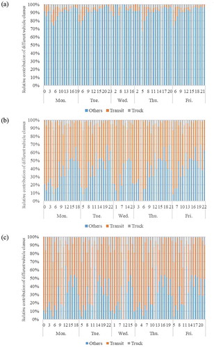
In Figure 7, we observe that across one week, the highest proportion (approximately 91%) of total CO concentrations comes from light-duty vehicles. Meanwhile, transit buses and trucks contribute about 6% and 3% of total CO concentrations, respectively. In contrast, transit buses contribute the majority of total NO_x and EC concentrations, with 59% and 61%, respectively. Approximately 37% and 30% of total NO_x and EC concentrations are estimated to come from other vehicles. In general, trucks were found to generate a relatively small proportion of NO_x or EC concentrations on our study segment, with percentages of 4% and 9%.

In addition, the diurnal trends of all pollutants across weekdays were also examined (figures are presented in the supplement). The diurnal trends of concentrations from different vehicle classes and total concentrations were hourly averaged across the weekdays. The results indicate that the highest concentrations occurred during the afternoon peaks when there were high traffic volumes on the network. It is important to note that there is another peak concentration period observed between 7 p.m. and 9 p.m. as the wind direction was almost orthogonal to the receptor and the wind brought pollutants towards the receptor.

Other vehicles were found to dominate the changes of CO concentrations across the study period on the segment. Besides, there were more fluctuations in NO_x and EC concentrations, since both transit bases and other vehicles influence these two pollutants. For instance, although there were less light-duty vehicles running on the study segment around midnight, the concentrations of NO_x and EC concentrations were still relatively high due to the operation of night buses.

Effect of transit buses on total emissions

In light of the large contribution of the transit buses to total emissions and near-road concentrations of NO_x and EC, the average EF of transit buses and the fleet averaged EF were calculated by dividing total emissions by the corresponding total number of vehicles and total traveled distance for these vehicles. The fleet average considers all vehicle classes except for transit buses, and its EF is a weighed value according to the proportion of each vehicle type. Per passenger emissions for transit buses and private vehicles were also calculated by averaging total emissions by the number of people in the corresponding vehicles. Ridership data for the College Street transit bus were obtained from the Toronto Transit Commission (Toronto Transit Commission Ridership and Cost Statistics for Bus and Streetcar Routes 2012; Toronto Transit Commission 2012), whereas the average number of passengers on private vehicles (passenger cars and passenger trucks) was assumed to be 1.6 according to the Canadian Vehicle Survey (Natural Resources Canada 2009).

In Table 1, we observe that each transit bus emits much more than the fleet average, as the ratios of EFs between transit bus and fleet average are always larger than 1 for different pollutants. This is expected, since EFs are normalized on a per vehicle basis. This comparison, however, illustrates the magnitude of transit bus emissions compared with the fleet average. In particular, each transit bus is estimated to produce NO_x and EC up to 70 times and 126 times the fleet average. This finding supports our previous observation that the largest contribution of total NO_x and EC emissions comes from transit buses (Contribution of trucks, transit buses, and other vehicles to total emissions).

Table 1. Ratios of EFs between transit bus and fleet average, and ratios of per passenger emissions between transit bus and private vehicles.

	Ratios of EFs (g/vkt) between transit bus and fleet average		Ratios of per passenger emissions (g/pkt) between transit bus and private vehicles
Pollutant	Thursday	Sunday	Thursday	Sunday
CO	2.2, 2.1 (1.1–3.5)	2.2, 2.1 (1.5–3.6)	0.19, 0.16 (0.06–0.43)	0.19, 0.14 (0.03–0.68)
NOx	68.0, 64.5 (32.6–126.6)	69.8, 67.0 (49.1–118.7)	7.29, 5.97 (2.30–17.22)	7.45, 5.93 (1.11–26.49)
EC	89.7, 73.9 (27.1–235.7)	125.7, 115.4 (25.1–232.9)	15.11, 13.13 (5.66–31.41)	21.48, 13.27 (2.54–84.68)

Notes. In the first line of each cell, the number in bold is the average value and the second number is the median; the numbers in the second line indicate the range.

vkt: vehicle kilometers traveled

pkt: passenger kilometers traveled

Furthermore, per passenger emission results reveal that generally a transit bus emits CO roughly 80% less than a private vehicle. Moreover, our results indicate that on a gram per passenger kilometer traveled (PKT) basis, a transit bus emits NO_x and EC up to 8 times and 22 times as much as a private vehicle. Lastly, we found that both ratios are always larger on Sunday than Thursday, which indicates that transit buses are relatively more efficient on Thursday, when ridership is higher.

Comparison of near-road air quality results

The concentrations of NO_x and CO were simulated based on traffic emissions calculated using modeled and plume-based EFs. In both cases, we employed estimated traffic emissions as the inputs and concentrations measured at the rooftop level as urban background concentrations.

Figure 8 presents the hourly distributions of simulated concentrations for the two pollutants based on modeled emissions as well as plume-based emissions, and measured concentrations at street level. Note that the dispersion model was implemented for the period extending from June 20 to June 24, 2016.

Figure 8. Box plots of hourly concentrations derived from emission model and plume-based method, as well as measured concentrations at street level, for two pollutants: (a) distribution of hourly nitrogen oxide (NO_x) concentrations; (b) distribution of hourly carbon monoxide (CO) concentrations. Boxes represent the interquartile range (25th to 75th percentiles), and whiskers indicate the minimum and maximum values. Dots indicate outliers, and crosses refer to mean values.

For both pollutants, simulated concentrations based on modeled emissions are higher than those based on the plume-based method. This is expected, since hourly EFs calculated using the emission model for both pollutants were higher than those derived from the plume-based approach (Comparison of emission factors).

In addition, the mean and median values of simulated NO_x concentrations derived from modeled emissions were 8% and 10% lower than the respective concentrations measured at street level, which are closer to the concentrations derived from the plume-based method, with mean and median values 18% and 20% lower than the measured concentrations. Observed NO_x concentrations have higher variability than simulated results.

Moreover, we observe that the mean simulated CO concentrations based on plume-based emissions is slightly closer (2% closer) to measured CO concentrations compared with simulated concentrations based on modeled emissions. On the other hand, the difference in median values between simulated results derived from modeled emissions and measured concentrations is 2%, which is smaller than the difference (11%) between simulated results based on the plume-based method and measured concentrations.

Overall, we found that simulated concentrations based on modeled emissions are generally closer to measured concentrations in terms of mean and median values as compared with concentrations derived from the plume-based method.

Conclusion and recommendations for future studies

This study aims at comparing estimates of EFs generated from MOVES and plume-based measurements along a busy urban corridor in downtown Toronto. In addition, the contributions of vehicle classes to various pollutants were evaluated using MOVES to highlight the high emitters and explore the potential explanations for the differences in EF estimates based on MOVES and plume-based methods. Finally, a street-canyon dispersion model was employed to determine the effects of differences in EFs on the resulting estimates of near-road air pollution.

We compared the fleet averaged EFs of NO_x and CO derived from the emission model with the EFs calculated using real-world measurements. The EFs derived from the model for all pollutants on weekends were generally within the range of their EFs on weekdays. In contrast, the EFs estimated using the plume-based method for NO_x were much higher on weekdays than on weekends, and the range of CO EFs on weekends was within the range of the EFs on weekdays.

Moreover, we observe significant differences in EFs for CO and NO_x between modeled and plume-based methods. The modeled EFs for CO and NO_x are about 2 times as high as plume-based EFs. This is consistent with previous studies indicating that the plume-based method tends to underestimate CO and NO_x EFs due to many factors, such as instrument sensitivity, differences of dilution rates between pollutants and CO₂, and local meteorology (Wang et al. 2015). More importantly, EFs derived from the plume-based method in this study represent vehicles passing the mid-block on College Street, which do not capture vehicle acceleration, deceleration, and idling when they are close to the intersection.

In order to investigate the influence of vehicle classes to different pollutants on the study segment, the total emissions and proportions of emissions from trucks, transit buses, and other vehicles were estimated for the same network with transit bus service versus streetcars. The results of the transit bus network reveal that the largest proportion of CO emissions comes from light-duty vehicles, whereas transit bus emissions account for approximately 60% and 70% of the total NO_x and EC, respectively. Meanwhile, trucks contribute a relatively small portion of the total emissions for all pollutants. For the streetcar network, all vehicle classes excluding trucks contribute more than 95% of the total CO emissions, as well as 85% and 70% of the total emissions of NO_x and EC, respectively.

The concentrations generated from different vehicle classes were estimated using a street-canyon dispersion model based on emission results for the transit bus network. The results indicate that most CO concentrations come from light-duty vehicles, whereas NO_x and EC concentrations are influenced by light-duty vehicles and transit buses. In addition to the influence of traffic volume, we observe that ambient concentrations are also significantly influenced by wind direction.

The comparison of EFs between transit bus and fleet average demonstrate that each transit bus emits much larger amounts of NO_x and EC. In addition, we found that transit buses were more efficient for CO but less efficient for NO_x and EC when compared with private vehicles on a per passenger level. This finding is of crucial importance to the development of new public transit systems, which need to consider the efficiency of public transportation in terms of fuel consumption and air pollution.

In addition, the hourly distributions of simulated concentrations for CO and NO_x based on modeled and plume-based emissions as well as concentrations measured at street level show that generally, simulated concentrations based on modeled emissions were closer to measured concentrations at street level as compared with simulated concentrations derived from the plume-based method. The difference in estimated concentrations derived from the two methods is not as large as the difference in estimated emissions due to the influence of meteorology and of the urban background. It is important to note that background concentrations contribute significantly to street-level concentrations, since our study area is located in downtown Toronto and concentrations generated from vehicles on other links could affect our study area.

Our discussion is strongly tied to the findings of our study and highlights what we learned based on our analysis and how it informs future work. Regarding the estimates of emissions derived from the plume-based method, our study shows that one of the main limitations of this approach is the single-point measurement location at mid-block. We recommend that additional data collection points should be located along the study segment, especially closer to the intersection in order to capture the impact of stop-and-go traffic on real-world emissions in urban environments. In addition, we observed that the radar falls short of identifying all pertinent vehicles classes, which is a crucial factor affecting road emissions. Image-processing techniques and automatic vehicle classification would ensure more reliable fleet composition data. Moreover, license plate recognition and cross-checking against vehicle registry information would be ideal to improve our understanding of the contributions from different vehicles. Finally, improving instrument sensitivity will result in more accurate emission estimates especially for pollutants such as CO that are characterized by concentrations close to background levels (Franco et al. 2013).

We also stress the importance of accurate speed data, especially that our corridor is on an arterial road. For example, we noted that drivers along College Street are more aggressive in reality compared with the output of the traffic simulation model; therefore, we calibrated the speed distribution in the model. The reliability of emission estimates based on the emission model was improved by calibrating the speed profiles derived from the traffic simulation model. Ideally, Global Positioning System (GPS) data would also be used to ascertain that the acceleration-deceleration profiles generated by the traffic simulation model are representative of local conditions. Furthermore, we noted various limitations to the radar performance, and we suggest that radar systems should be positioned on both sides of the road to provide better quality control given that radar performance decreases with the increase in the distance from the traffic lane. Lastly, measurement campaigns in different seasons could enable us to conduct temporal and seasonal analysis of EFs based on these two methods.

Supplementary Material

Supplemental data for this paper can be accessed on the publisher’s website.

Additional information

Notes on contributors

Junshi Xu

Junshi Xu is a Ph.D. candidate in the Department of Civil & Mineral Engineering at the University of Toronto.

Jonathan Wang

Jonathan Wang and Nathan Hilker are Ph.D. candidates in the Department of Chemical Engineering and Applied Chemistry at the University of Toronto.

Masoud Fallah-Shorshani

Masoud Fallah-Shorshani is a Post-doctoral fellow in the Department of Civil & Mineral Engineering at the University of Toronto.

Marc Saleh

Marc Saleh is a M.Sc. candidate in the Department of Civil & Mineral Engineering at the University of Toronto.

Ran Tu

Marc Saleh is a M.Sc. candidate in the Department of Civil & Mineral Engineering at the University of Toronto.

Christos Stogios

Ran Tu, An Wang and Laura Minet are Ph.D. candidates in the Department of Civil & Mineral Engineering at the University of Toronto.

Greg Evans

Christos Stogios is a M.Sc. graduate from the Department of Civil & Mineral Engineering at the University of Toronto.

Marianne Hatzopoulou

Greg Evans is a professor in the Department of Chemical Engineering and Applied Chemistry at the University of Toronto. He is the director of the Southern Ontario Center for Atmospheric Aerosol Research (SOCAAR), which is an interdisciplinary centre for the study of air quality, with a focus on how aerosols impact human health and the environment.

Marianne Hatzopoulou is an associate professor in the Department of Civil & Mineral Engineering at the University of Toronto. Her research area bridges between transportation and environmental analysis; and her main expertise is in modelling of road transport emissions and urban air quality as well as evaluating population exposure to air pollution. She is a Canada Research Chair in Transportation and Air Quality, and leads the Transportation and Air Quality (TRAQ) research group.

References

- Bai, S., M. McCarthy, A. Graham, and S. Shaw. 2016. Mobile source NOx emissions in the National Emissions Inventory. Retrieved from. https://register.extension.iastate.edu/images/events/TPAQ/presentations/19_Bai.PDF (accessed June 27, 2018).
- Bokare, P.S., and A.K. Maurya. 2013. Study of effect of speed, acceleration and deceleration of small petrol car on its tail pipe. Int. J Traffic Transp. Eng. 3(4):465–478. doi:10.7708/ijtte.2013.3(4).09.
- Carslaw, D.C., S.D. Beevers, J.E. Tate, E.J. Westmoreland, and M.L. Williams. 2011. Recent evidence concerning higher NOx emissions from passenger cars and light duty vehicles. Atmos. Environ. 45 (39): 7053–7063. doi: 10.1016/j.atmosenv.2011.09.063.
- Cheng, Y., S.C. Lee, K.F. Ho, J.C. Chow, J.G. Watson, P. K.K. Louie, J.J. Cao, and X. Hai. 2010. Chemically-speciated on-road PM2.5 motor vehicle emission factors in Hong Kong. Sci. Total Environ. 408(7):1621–1627. doi:10.1016/j.scitotenv.2009.11.061.
- Dallmann, T.R., T.W. Kirchstetter, S.J. Demartini, and R.A. Harley. 2013. Quantifying on-road emissions from gasoline-powered motor vehicles: Accounting for the presence of medium- and heavy-duty diesel trucks. Environ. Sci. Technol. 47(23):13873–13881. doi:10.1021/es402875u.
- Franco, V., M. Kousoulidou, M. Muntean, L. Ntziachristos, S. Hausberger, and P. Dilara. 2013. Road vehicle emission factors development: A review. Atmos. Environ 70: 84–97. doi:10.1016/j.atmosenv.2013.01.006.
- Fuertes, E., M. Standl, J. Cyrys, D. Berdel, A. Von Berg, C. Bauer, U. Kr, and D. Sugiri. 2013. A longitudinal analysis of associations between traffic-related air pollution with asthma. Allergies and sensitization in the GINIplus and LISAplus birth cohorts. PeerJ 1:e193. doi:10.7717/peerj.193.
- Gorjestani, A., A. Menon, P.-M. Cheng, C. Shankwitz, and M. Donath. 2008. The design of an optimal surveillance system for a cooperative collision avoidance system—Stop Sign Assist. CICAS-SSA Report 2. Retrieved from http://www.dot.state.mn.us/its/projects/2011-2015/cicas/CICAS-SSA%20Report%202.pdf (accessed June 27, 2018).
- Ježek, I., L. Drinovec, L. Ferrero, M. Carriero, and G. Močnik. 2015. Determination of car on-road black carbon and particle number emission factors and comparison between mobile and stationary measurements. Atmos. Meas. Tech. 8(1):43–55. doi:10.5194/amt-8-43-2015.
- Liu, B., and H.C. Frey. 2015. Variability in light-duty gasoline vehicle emission factors from trip-based real-world measurements. Environ. Sci. Technol. 49(20):12525–12534. doi:10.1021/acs.est.5b00553.
- Melorose, J., R. Perroy, and S. Careas. 2015. Statewide Agricultural Land Use Baseline 2015. Retrieved from http://hdoa.hawaii.gov/salub/ (accessed June 27, 2018).
- Natural Resources Canada. 2009. Canadian vehicle survey. Canada: Public Works and Government Services Canada (PWSGC).
- Natural Resources Canada. 2017. 2017 fuel consumption guide, 43. Canada: Public Works and Government Services Canada (PWSGC).
- Pérez-Martínez, P.J., R.M. Miranda, T. Nogueira, M.L. Guardani, A. Fornaro, R. Ynoue, and M.F. Andrade. 2014. Emission factors of air pollutants from vehicles measured inside road tunnels in São Paulo: Case study comparison. Int. J. Environ. Sci. Technol. 11(8):2155–2168. doi:10.1007/s13762-014-0562-7.
- Reyna, J.L., M.V. Chester, S. Ahn, and A.M. Fraser. 2015. Improving the accuracy of vehicle emissions profiles for urban transportation greenhouse gas and air pollution inventories. Environ. Sci. & Technol. 49(1):369–376. doi: 10.1021/es5023575.
- Soulhac, L., P. Salizzoni, F. Cierco, and R. Perkins. 2011. The model SIRANE for atmospheric urban pollutant dispersion; Part I, presentation of the model. Atmos. Environ 45 (39): 7379–7395. doi: 10.1016/j.atmosenv.2011.07.008.
- Thunis, P., A. Miranda, J.M. Baldasano, N. Blond, J. Douros, A. Graff, S. Janssen, et al. 2016. Overview of current regional and local scale air quality modelling practices: Assessment and planning tools in the EU. Environ. Sci. Policy 65: 13–21. doi:10.1016/j.envsci.2016.03.013.
- Toronto Transit Commission 2012. Ridership and cost statistics for bus and streetcar routes, 2012, 1–4.
- U.S Enviromental Protection Agency. 2015a. Exhaust emission rates for heavy-duty on-road vehicles in MOVES2014 exhaust emission rates for heavy-duty on-road vehicles in MOVES2014. https://nepis.epa.gov/Exe/ZyPDF.cgi?Dockey=P100NO46.pdf (accessed June 27, 2018).
- U.S. Environmental Protection Agency. 2015b. Exhaust emission rates for light-duty on-road vehicles in MOVES2014 final report. https://nepis.epa.gov/Exe/ZyPDF.cgi?Dockey=P100NNVN.pdf (accessed June 27, 2018).
- Wang, A., Y. Ge, J. Tan, M. Fu, A.N. Shah, Y. Ding, H. Zhao, and B. Liang. 2011a. On-road pollutant emission and fuel consumption characteristics of buses in Beijing. J. Environ. Sci. 23 (3): 419–426. doi: 10.1016/S1001-0742(10)60426-3.
- Wang, D. Westerdahl, Y. Wu, X. Pan, and K.M. Zhang. 2011b. On-road emission factor distributions of individual diesel vehicles in and around Beijing, China. Atmos. Environ. 45(2):503–513. doi:10.1016/j.atmosenv.2010.09.014.
- Wang, J.M., C.H. Jeong, N. Zimmerman, R.M. Healy, D.K. Wang, F. Ke, and G.J. Evans. 2015. Plume-based analysis of vehicle fleet air pollutant emissions and the contribution from high emitters. Atmos. Tech. 8(8):3263–3275. doi:10.5194/amt-8-3263-2015.
- Weiss, M.,P. Bonnel, R. Hummel, U. Manfredi, R. Colombo, G. Lanappe, P. Lelijour, and M. Sculati. 2011. Analyzing On-Road Emissions of Light-Duty Vehicles with Portable Emission Measurement Systems (PEMS). European Commission Joint Research Centre Technical Report EUR 24697 EN.
- Yu, X., P. Prevedouros, and G. Sulijoadikusumo. 2010. Evaluation of autoscope, smartsensor HD, and infra-red traffic logger for vehicle classification. Transp. Res. Rec. J. Transp. Res. Board 2160:77–86. doi:10.3141/2160-09.
- Zhao, H., R. Stone, and L. Zhou. 2010. Analysis of the particulate emissions and combustion performance of a direct injection spark ignition engine using hydrogen and gasoline mixtures. Int. J. Hydrogen Energy 35 (10): 4676–4686. doi: 10.1016/j.ijhydene.2010.02.087.
- Zimmerman, N., J.M. Wang, C. Jeong, J.S. Wallace, and G. J. Evans. 2016. Assessing the climate trade-offs of gasoline direct injection engines. Environ. Science & Technol. doi:10.1021/acs.est.6b01800.