Future year ozone source attribution modeling study using CMAQ-ISAM

ABSTRACT

To achieve the current United States National Ambient Air Quality Standards (NAAQS) attainment level for ozone or particulate matter, current photochemical air quality models include tools to determine source apportionment and/or source sensitivity. Previous studies by the authors have used the Ozone and Particulate Matter Source Apportionment Technology and Higher-order Decoupled Direct Method probing tools in CAMx to investigate these source-receptor relationships for ozone. The recently available source apportionment for CMAQ, referred to as the Integrated Source Apportionment Method (ISAM), was used in this study to conduct future year (2030) source attribution modeling. The CMAQ-ISAM ozone source attribution results for selected cities across the U.S. showed boundary conditions were the dominant contributor to the future year highest July maximum daily 8-hour average (MDA8) ozone concentrations. Point sources were generally larger contributors in the eastern U.S. than in the western U.S. The contributions of on-road mobile emissions were around 5 ppb at most of the cities selected for analysis. Off-road mobile source contributions were around 20 ppb or nearly 30%. Since boundary conditions play an important role in future year ozone levels, it is important to characterize future year boundary conditions accurately. The current implementation of ISAM in CMAQ 5.0.2 requires significant computing resources for ozone source attribution, making it difficult to conduct long-term simulations for large domains. The computing requirements for PM source attribution are even more onerous. CMAQ 5.2 was released after this study was completed, and does not include ISAM. If an efficient version of ISAM becomes available, it could be used in long-term ozone and PM2.5 studies. Implications: Ozone source attribution results provide useful information on important emission source contribution categories and provide some initial guidance on future emission reduction strategies. This study explains a new source apportionment technique, CMAQ-ISAM, and compares it to CAMx OSAT. The techniques have similar results: ozone’s highest source contributor is boundary conditions, followed by point sources, then off-road mobile sources. The current version of ISAM in CMAQ 5.0.2 requires significant computing resources for ozone source attribution, while the computing requirements for PM source attribution are even more onerous. CMAQ 5.2 was released after this study was completed, and does not include ISAM.

Introduction

Regulatory agencies use air quality models to determine compliance with the National Ambient Air Quality Standards (NAAQS). Currently, agencies are planning strategies for attainment of ozone (O₃) and particulate matter (PM) NAAQS. In order to develop appropriate emission control strategies, it is useful to determine which emission sources are contributing to these pollutants. Current photochemical air quality models, such as the Comprehensive Air Quality Model with Extensions (CAMx) (ENVIRON 2011) and the U.S. Environmental Protection Agency’s (EPA) Community Multiscale Air Quality (CMAQ) (Byun and Schere 2006; Foley et al. 2010) include tools (sometimes referred to as probing tools or instrumented tools) to determine source apportionment and/or source sensitivity. These tools are increasingly being used to help understand complex air quality issues (e.g., Wagstrom et al. 2008; Wang et al. 2009; Burr and Zhang 2011; Baker and Kelly 2014; Collet et al. 2014a; Goldberg et al. 2016; Karamchandani et al. 2017).

Previous studies by the authors have used the Ozone and Particulate Matter Source Apportionment Technology (OSAT/PSAT) and Higher-order Decoupled Direct Method (HDDM) probing tools in CAMx to investigate these source-receptor relationships for ozone (Collet et al. 2017). Until recently, CMAQ did not include a source apportionment tool similar to the OSAT tool in CAMx. Previous versions of CMAQ required the use of a brute force approach to calculate source contributions. This approach involves zeroing out emissions from a particular source or source category and determining its contribution by subtracting the zero-out run results from the results of a base run with all source categories. This is resource-intensive and results in a large change in the chemical environment between the base run and zero-out run. Thus, it can be considered a sensitivity study rather than a true source apportionment. Furthermore, the sum of source contributions from the zero-out method does not equal the ozone estimates from all sources combined for nonlinear systems (Yarwood et al. 1996). The availability of a source apportionment tool in a recent version of CMAQ (CMAQ 5.0.2) provides an opportunity to compare results from two different source apportionment approaches in two different models. The CMAQ source apportionment method, referred to as the Integrated Source Apportionment Method (ISAM) (Kwok et al. 2015; Kwok, Napelenok, and Baker 2013), was used in this study, and the results were compared with previous source apportionment modeling studies conducted with CAMx (Collet et al. 2017).

Comparison of source apportionment approaches

Like the OSAT/PSAT source apportionment tools in CAMx, the ISAM tool provides a method for estimating the contributions of multiple source areas, categories, and pollutant types to ozone and PM formation in a single model run, which is an advantage over the zero-out approach when a large number of source attribution studies need to be conducted. The ISAM source apportionment for PM species was initially implemented by Kwok, Napelenok, and Baker (2013), and the approach was later extended to ozone and its precursors, nitrogen oxides (NO_x) and volatile organic compounds (VOCs) (Kwok et al. 2015). The ISAM source apportionment tool is different from OSAT/PSAT for horizontal advection and solving chemical equations. For the horizontal advection, ISAM explicitly handles individual source tracers whereas PSAT apportions the source group to the total advection fluxes. To solve chemical reactions related to tagged source tracers, ISAM solves host model concentrations before updating source group concentrations. Then ISAM prepares a two-dimensional Jacobian matrix for each tagged source, which is associated with two lists of total host model concentrations; the two lists are the concentrations before and after each time step. This Jacobian matrix is used to update a tagged source group’s concentrations and allows ISAM to explicitly calculate individual species rather than lumped species. The ISAM ozone source apportionment uses similar chemistry-related assumptions as used in CAMx-OSAT. To determine whether a grid cell belongs to a NO_x- or VOC-limited regime, ISAM uses the ratio of the production rate of hydrogen peroxide (H₂O₂) to the production rate of nitrate (NO₃), or PH₂O₂/PNO₃. If this ratio is larger than 0.35, the grid cell is assumed to be NO_x-limited, and VOC-limited otherwise. Like OSAT, ISAM also ignores the destruction (scavenging) of ozone by nitric oxide (NO) because it is part of a null cycle and ozone is recovered very quickly. To attribute contributions of ozone to specific source groups, the host model ozone production rate is multiplied by the fraction of individual source group’s NO_x- or MIR (maximum incremental reactivity)-weighted VOCs over total NO_x or total MIR-weighted VOCs.

As mentioned above, ISAM differs from OSAT in its handling of tracer species. OSAT lumps VOC species after weighting with MIR and calls this a VOC family. Instead of multiple VOC species, only one VOC family is used as a tracer species to reduce computational costs in OSAT. Therefore, VOC decay and contributions to ozone production are also handled with the one tracer species. On the other hand, ISAM explicitly handles individual source tracers. Thus, CMAQ-ISAM requires substantial computing resources, and an ozone-only source attribution simulation with ISAM is about an order of magnitude slower than a CAMx source attribution for both ozone and PM with OSAT/PSAT. With PM source attribution, the CMAQ-ISAM simulation times were much longer and impractical. Without tagging PM tracers (i.e., ozone source attribution only), the CMAQ-ISAM simulation took nearly 1 day of real time for each day of simulation time with 54 CPUs (central processing units) (6 × 9 MPI [message passing interfaces]) of Intel Xeon CPU E5-2690 v4 at 2.60 GHz. In contrast, the CAMx OSAT/PSAT (i.e., both ozone and PM source attribution) simulations are more than 10 times faster for a similar computing configuration. With PM source attribution, the CMAQ-ISAM simulation times were much longer and impractical for this study. Thus, for this study, only a summer month (July) simulation for ozone was performed with CMAQ-ISAM. However, full base year and future year simulations with CMAQ without ISAM were conducted to develop future year design values of ozone for comparison with CAMx-predicted future year design values (Collet et al. 2014b).

Modeling approach

The EPA’s CMAQ model (Byun and Schere 2006; Foley et al. 2010) version 5.0.2 with the ISAM source apportionment tool (Kwok et al. 2015; Kwok, Napelenok, and Baker 2013) was used to calculate future year source attributions for ozone concentrations in the contiguous United States (U.S.) for various source categories for the month of July. In addition, future year annual CMAQ simulations were conducted without the ISAM probing tool to calculate future year design values (DVFs). Future year CMAQ runs used meteorology for the 2011 base year, future year anthropogenic emissions, and base year boundary conditions (BCs) and natural, i.e., biogenic and fire, emissions. In addition, a 2011 base year annual simulation was conducted for model performance evaluation purposes.

The modeling domain was the same as used in the CAMx source attribution study of Collet et al. (2017). This domain, shown in Figure 1, is the 12US2 domain used by the EPA for its ozone assessment using the 2011-based air quality modeling platform (EPA 2015). The domain covers the 48 contiguous states (CONUS) as well as the southern portions of Canada and the northern portions of Mexico. EPA’s Weather Research and Forecasting (WRF) outputs were used to develop the model-ready meteorological fields. Details of EPA’s annual 2011 WRF simulation and evaluation are provided in a technical support document (EPA 2014a). The CMAQ-ready files were generated for the 2011 base year using the Meteorology-Chemistry Interface Processor (MCIP) version 4.2 (Otte and Pleim 2010), released in August 2013.

Figure 1. CONUS 12 km CAMx modeling domain (from EPA 2015).

Results from the global atmospheric chemistry model, GEOS-Chem, provided by EPA, were used to specify the lateral boundary and initial conditions for model species. The global GEOS-Chem model simulates atmospheric chemical and physical processes driven by assimilated meteorological observations from National Aeronautics and Space Administration’s (NASA) Goddard Earth Observing System (GEOS). The EPA ran the model for 2011 with a grid resolution of 2.0° by 2.5° in latitude-longitude coordinates (EPA 2015). GEOS-Chem outputs were first converted to CMAQ format using an EPA processor (Henderson et al. 2014) that maps the GEOS-Chem species to CMAQ species (based on the CB05 chemistry mechanism). Previous studies (e.g., Johnson et al. 2015; Kemball-Cook et al. 2015) for the Texas Commission on Environmental Quality (TCEQ) have suggested that ozone is overestimated in the GEOS-Chem output. Thus, following the method adopted by the TCEQ in its regional photochemical modeling applications, in the final step of creating the CMAQ-ready boundary conditions, ozone concentrations were reduced by 5 ppb for all boundary cells and an additional 10 ppb for boundary grid cells for the Caribbean and Gulf of Mexico (GoM). Various caps were also applied to ozone precursors over the Atlantic Ocean and GoM to deplete the ozone coming onshore, as described in Kemball-Cook et al. (2015) and shown in Table 1.

Table 1. Maximum concentration limits for ozone precursors applied to the 36 km lateral boundary condition grid cells across the Gulf of Mexico, Caribbean Sea, and the Atlantic Ocean south of Cape Hatteras (from Kemball-Cook et al. 2015).

CAMx species	Description	Maximum concentration (ppb)
NO2	Nitrogen dioxide	0.05
CO	Carbon monoxide	150.0
N2O5	Dinitrogen pentoxide	0.001
HNO3	Nitric acid	0.25
PNA	Peroxynitric acid	0.001
H2O2	Hydrogen peroxide	0.5
NTR	Organic nitrates	0.01
FORM	Formaldehyde	0.25
ALD2	Acetaldehyde	0.05
ALDX	Propionaldehyde and higher aldehydes	0.02
PAR	Paraffin carbon bond (C–C)	1.0
OLE	Terminal olefin carbon bond (R–C=C)	0.01
ETHA	Ethane	1.0
MEPX	Methylhydroperoxide	0.1
PAN	Peroxyacetyl nitrate	0.01
INTR	Organic nitrates from ISO2 reaction with NO	0.001
ISOP	Isoprene	0.1
ISPD	Isoprene product (lumped methacrolein, methyl vinyl ketone, etc.)	0.1
TERP	Monoterpenes	0.05
ISP	Isoprene (SOA chemistry)	0.1
TRP	Monoterpenes (SOA chemistry)	0.05
TOL	Toluene and other monoalkyl aromatics	0.02
XYL	Xylene and other polyalkyl aromatics	0.01
SO2	Sulfur dioxide	0.1
PRPA	Propane	0.5
ACET	Acetone	0.25
KET	Ketone carbon bond (C=O)	0.05
BENZ	Benzene	0.1

EPA’s 2011v6.2 air quality modeling platform emissions formed the framework for this study. This includes all the emission inventories and ancillary data files used for emission modeling. The 2011v6.2 modeling platform is based on the 2011 National Emissions Inventory (NEI). In July 2015, the EPA provided a Notice of Data Availability (NODA) for the 2011v6.2 modeling platform and 2011 inventory data files. Many emission inventory components of this air quality modeling platform are based on the 2011 National Emissions Inventory, version 2 (2011NEIv2). The EPA developed the 2011v6.2 platform to support ozone transport modeling for the 2008 NAAQS, the 2015 NAAQS for ozone, and other special studies.

For this study, unmerged air quality model–ready emission components were obtained from the EPA for the 2011 base case and 2025 projection scenarios. This study’s 2011 base case emissions are based on the 2011 base case emissions in the 2011v6.2 modeling platform. As mentioned above, the EPA 2011 base case emissions are mostly based on the 2011NEIv2 inventory. The 2011NEIv2 includes on-road mobile emissions for 2011 that were developed using the EPA’s Motor Vehicle Emission Simulator (MOVES2014) for all contiguous states except California; for California, it uses the California Air Resources Board’s (CARB) Emission Factors (EMFAC) models. The modeling platform emissions were generated by the EPA in a format that is compatible with CMAQ 5.0.2. However, the EPA processed emissions in terms of the Carbon Bond version 6 revision 2 (CB6r2) chemical mechanism used by CAMx, which is currently not available in CMAQ. CMAQ is available with the Carbon Bond 2005 (CB05) chemical mechanism. The CB6 to CB05 mapping is shown in Table2.

Table 2. CB05 to CB6 mapping.

CB05 species	CB6 species
ALD2	ALD2
ALDX	ALDX
BENZENE	BENZ
CH4	CH4
CO	CO
ETH	ETH
ETHA	ETHA
ETOH	ETOH
FORM	FORM
IOLE	IOLE
ISOP	ISOP
MEOH	MEOH
NROG	NROG
NVOL	NVOL
OLE	OLE
PAR	PAR + 3ACET + BENZ + ETHY + KET + 1.5PRPA
SESQ	SQT
TERP	TERP
TOL	TOL
UNR	UNR
XYL	XYL

As in our previous CAMx source attribution study (Collet et al. 2017), only the anthropogenic sectors from the 2011v6.2 platform were used and the natural source category emissions were developed. Emissions for the natural source categories were developed using the 2011 meteorological data and models for the 12 km (12US2) domain in a format suitable for CMAQ. Biogenic emissions were developed using the Model of Emissions of Gases and Aerosols from Nature (MEGAN) (Guenther et al. 2012; Wiedinmyer et al. 2007) using the 2011 meteorology from WRF. MEGAN was configured to generate biogenic emissions in CMAQ format for the CB05 mechanism. Although MEGAN is a well-accepted model, it has been shown to overestimate isoprene emissions (e.g., Goldberg et al. 2016; Kota et al. 2015; Wang et al. 2017). In areas that are VOC-limited, this overestimation is likely to increase the attribution of biogenic emissions to ozone. However, most areas in our modeling domain are NOx-limited, and Zhang et al. (2017) have shown that source apportionment methods, such as OSAT or ISAM, tend to apportion less ozone to biogenics as biogenic VOC (BVOC) emissions increase, since that shifts marginal ozone formation toward more NO_x-limited conditions.

Sea salt emissions were developed using an emission processor that integrates published sea spray flux algorithms to estimate sea salt PM emissions. The forest fire emissions were based on 2011 calendar year estimates of satellite-based fire emissions from the National Center for Atmospheric Research (NCAR) Fire INventory (FINN). Each fire record was treated as a point source, and emissions were distributed vertically into multiple model layers to better represent each fire plume.

The 2025 CMAQ-ready emissions provided by the EPA were used for the future year (2030) emissions. Future year emissions from the natural source categories were assumed to be the same as the 2011 base year emissions. The 2030 emissions for all anthropogenic source categories, except on-road mobile sources, were assumed to be the same as the case of EPA’s 2025 emissions. The on-road mobile emissions for 2030 were developed using MOVES2014 and the CARB EMFAC 2014 model over the CONUS domain. NO_x emissions from on-road sources were projected to decrease from nearly 6 million tons per year in 2011 to slightly over 1 million tons per year in 2030, whereas the projected reductions in VOC emissions from on-road sources were over 2 million tons—from nearly 3 million tons per year in 2011 to about 600,000 tons per year in 2030.

MOVES2014 was run in inventory mode using default MOVES inputs to develop on-road mobile emissions for all contiguous U.S. states, except California. The emission rates were seasonal, representing one winter month (January) and one summer month (July) in 2030. The grams-per-mile and grams-per-vehicle emission rates were generated by Source Classification Codes (SCC). The 2011 vehicular activity data, such as population and vehicle miles traveled (VMT), were obtained from the 2011v6.2 modeling platform. The 2011 activity data were then projected to the future year (2030). The activity projection factors were based on the growth assumptions within MOVES2014 and were used to project vehicle activity inputs (VMT and population) from 2011 to 2030. Grams-per-mile and grams-per-vehicle emission rates were multiplied by the projected VMT and population, respectively, to obtain the 2030 on-road inventory. The MOVES2014 outputs for 2030 on-road emissions were formatted for use in the Sparse Matrix Operator Kernel Emissions (SMOKE) modeling system, an emission processing system designed to create gridded, speciated, hourly emissions for input into a variety of air quality models, including CMAQ. July emissions were used for the summer season, January emissions for the winter season, and the average of the summer and winter months for the spring and fall seasons.

For California, the EMFAC 2014 model was used to generate 2030 statewide emissions. All model default inputs were used to estimate 2030 emissions by county, fuel type, and vehicle type. The model generated emissions for all criteria pollutants, including brake and tire wear. The EMFAC 2014 model outputs were also formatted for input to SMOKE. The latest EMFAC 2014 model incorporates the following CARB/federal regulations: Advanced Clean Car regulation, Assembly Bill No. 1493 (Pavley) regulation, On-Road Heavy-Duty Diesel Vehicles (In-Use) regulation, Heavy-Duty Phase I Green House Gas (GHG) regulation, CARB Heavy-Duty Tractor-Trailer GHG regulation. Then the 2030 on-road emissions were processed through the SMOKE modeling system to generate gridded, hourly, model-species emission inputs for CMAQ.

The final step in developing the model-ready emissions was to combine sector-specific gridded, speciated, hourly emissions together to create CMAQ-ready emissions. The EPA-provided 2011v6.2 platform emissions for the CB6r2 chemical mechanism were converted to the CB05 chemical mechanism for CMAQ.

Model performance evaluation

A model performance evaluation (MPE) is a necessary component of any modeling exercise, since it provides confidence in the use of the model for investigating emission control scenarios. An operational model performance evaluation was performed in which CAMx estimates of ozone concentrations for the 2011 simulation period was compared with observed values. The procedures for the model performance evaluation were based on guidance from the EPA (EPA 1991, 2001, 2007, 2014b) and experience in CAMx modeling (e.g., Morris et al. 2009a, 2009b). CAMx performance was for the 12US2 modeling domain using ozone observations from the Air Quality System (AQS) monitoring network. The ozone model performance evaluation was limited to the ozone season (April through October 2011). For both CMAQ and CAMx, there is generally good agreement between the modeled and observed temporal variabilities and meets performance goals, as shown by the overall model performance statistics in Table 3.

Table 3. CMAQ and CAMx model performance statistics for MDA8 ozone concentrations for April–October 2011.

April–October MDA8 ozone statistics	CMAQ 12 km	CAMx 12 km
Fractional bias (%)	−10	−7
Fractional gross error (%)	15	14
Normalized mean bias (%)	−9	−6
Normalized mean error (%)	14	14
Mean normalized bias (%)	−8	−5
Mean normalized gross error (%)	14	13
Mean bias (ppb)	−5	−3
Mean absolute gross error (ppb)	8	7
Number of stations	1321	1321

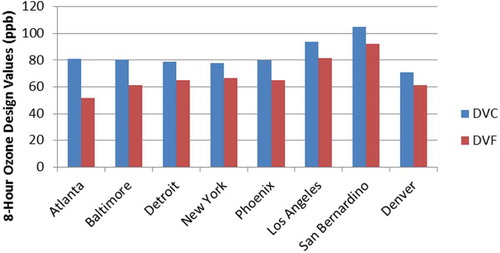
The base year simulations were conducted primarily for model evaluation and to develop a baseline for the future year calculations. A comparison of base year and future year ozone design values is shown in Figure 2 for the CMAQ simulations. The comparisons for CAMx are qualitatively similar.

Figure 2. 2011 Design Value Current (DVC) and 2030 Design Value Future (DVF) 8-hr ozone design values at selected monitoring locations over the U.S. from the CMAQ results.

Source apportionment results and analysis

The ozone source apportionment results from the CMAQ-ISAM simulation for July 2030 were compared with results from CAMx-OSAT source attribution results for the same period. The results are shown for the first highest MDA8 ozone concentrations at selected locations. Figure 3 shows the contributions of various source categories to future year (2030) first highest MDA8 ozone concentrations during July at 12 monitoring locations in various cities in the western and eastern U.S. Absolute contributions (in ppb) estimated by CMAQ-ISAM are shown in the top panel, whereas the middle panel shows the corresponding estimates from CAMx-OSAT. The bottom panel shows the relative contributions from the two source attribution approaches.

Figure 3. Future year (2030) contributions by source category to first highest July MDA8 ozone concentrations at 12 locations in the western and eastern U.S. The top panel shows CMAQ-ISAM–estimated absolute contributions, the middle panel shows CAMx-OSAT–estimated absolute contributions, and the bottom panel shows the relative source contributions for the two source attribution approaches.

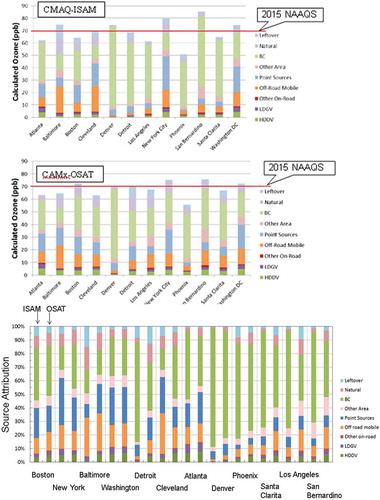
Both the CMAQ and CAMx source attribution tools estimate that boundary conditions are the dominant contributors at the selected locations in the western U.S. and are also important for many of the selected eastern U.S. locations. From the CMAQ results, we see that at all but three locations the boundary condition contributions are more than 25%, and more than 85% at the Denver location. At three locations, Baltimore, Cleveland, and New York City, boundary condition contributions to the first highest MDA8 ozone value are around 15–20%. Point sources are a larger percentage of the total in the eastern U.S. than in the western U.S. Total on-road mobile source contributions are less than 10 ppb at all locations and less than 5 ppb at a majority of the selected locations. On-road heavy-duty diesel vehicle (HDDV) contributions are generally higher than on-road light-duty gasoline vehicle (LDGV) contributions, whereas the contributions from other on-road source categories (primarily LDDV and HDGV) are small, as noted in previous year studies. The largest off-road contribution (20 ppb or nearly 30%) is at the Baltimore location, followed by contributions between 10 and 20 ppb at the Cleveland, New York City, and Washington, DC, locations.

The CAMx-OSAT trends are similar to the CMAQ-ISAM results. The boundary conditions are dominant contributors for most of the locations, point sources are more important in the eastern U.S. than in the western U.S., on-road mobile sources contribute less than 10 ppb at all locations, and the largest off-road contribution is at the Baltimore location with a similar magnitude of contribution. However, there are some subtle differences between the CMAQ-ISAM and CAMx-OSAT results. CMAQ predicts first highest MDA8 ozone concentrations that are higher than CAMx at five locations (Baltimore, Cleveland, Denver, New York City, and San Bernardino) by 5–10 ppb, whereas CAMx predicts higher values than CMAQ at four locations (Boston, Los Angeles, Phoenix, and Santa Clarita) by 3–7 ppb. For the Atlanta, Detroit, and Washington, DC, locations, both models agree within 2 ppb. CMAQ predicts higher boundary conditions contributions at Detroit and Los Angeles than CAMx. CMAQ predicts higher off-road contributions than CAMx at Cleveland, whereas CAMx predicts higher off-road contributions than CMAQ at Detroit and Los Angeles.

Conclusion

CMAQ-ISAM was used to conduct future year (2030) source attribution modeling for comparison with previous studies using the CAMx source attribution tools. Because of the extremely high computational (memory, disk, and CPU) requirements for running an ISAM simulation, the source attribution modeling was conducted for ozone only and one summer month (July) only. In addition to the 1-month ozone source attribution study, the base CMAQ (i.e., without ISAM) was used for conducting base year (2011) and future year simulations. These simulations provided the information required to forecast future year ozone design values.

The CMAQ-ISAM ozone source attribution results for selected cities across the U.S. showed that boundary conditions were the dominant contributor to the future year (2030) first highest July MDA8 ozone concentrations at the western U.S. locations and were also significant at many of the eastern U.S. locations. These results are generally consistent with the corresponding CAMx results. Point sources were generally larger contributors in the eastern U.S. than in the western U.S. The contributions of on-road mobile emissions were around 5 ppb at most of the cities selected for analysis and less than 10 ppb for all the locations. HDDV contributions were generally higher than LDGV contributions. HDGV and LDDV contributions were negligible. Off-road mobile source contributions were high (20 ppb or nearly 30%) at the Baltimore location and were also important at the Cleveland, New York City, and Washington, DC, locations. In general, the CMAQ-ISAM ozone source attribution results over the selected U.S. cities are similar to the CAMx-OSAT source attribution results.

Although there are some differences between the CMAQ and CAMx results, both models compare well overall with each other in terms of model performance, source attribution, and future year design values. Boundary conditions play an important role in future year ozone levels, suggesting that air quality in future years will be influenced to a large extent by inflow of pollution from outside the U.S. Thus, it is important to characterize future year boundary conditions more accurately. On-road mobile emissions contribute less than 10 ppb to ozone levels in most areas, with HDDV emissions being the largest contributor.

The current implementation of ISAM in CMAQ 5.0.2 requires significant computing resources for ozone source attribution, making it difficult to conduct long-term simulations for large domains. The computing requirements for PM source attribution are even more onerous. CMAQ 5.2 was released after this study was completed, but the current version of the release does not include ISAM. If an efficient version of ISAM becomes available in future versions of CMAQ, it could be used in future long-term (annual) studies for both ozone and PM_2.5.

Additional information

Notes on contributors

Susan Collet

Susan Collet is an Executive Engineer in the Product Regulatory Affairs division at Toyota Motor North America, Inc., in Ann Arbor, Michigan.

Toru Kidokoro

Toru Kidokoro is a Development Manager in the Advanced Powertrain Management System Development Division at Toyota Motor Corporation in Shizuoka, Japan.

Prakash Karamchandani

Prakash Karamchandani is a Managing Consultant in the Air Sciences Division at Ramboll U.S. Corporation in Novato, California.

Jaegun Jung

Jaegun Jung is a Senior Consultant in the Air Sciences Division at Ramboll U.S. Corporation in Novato, California.

Tejas Shah

Tejas Shah is a Managing Consultant in the Air Sciences Division at Ramboll U.S. Corporation in Novato, California.

References

- Baker, K. R., and J. T. Kelly. 2014. Single source impacts estimated with photochemical model source sensitivity and apportionment approaches. Atmos. Environ. 96:266–274. doi:10.1016/j.atmosenv.2014.07.042.
- Burr, M. J., and Y. Zhang. 2011. Source apportionment of fine particulate matter over the Eastern U.S. Part II: Source apportionment simulations using CAMx/PSAT and comparisons with CMAQ source sensitivity simulations. Atmos. Pollut. Res. 2:318–336. doi:10.5094/APR.2011.037.
- Byun, D., and K. L. Schere. 2006. Review of the governing equations, computational algorithms, and other components of the Models-3 Community Multiscale Air Quality (CMAQ) modeling system. Appl. Mech. Rev. 59:51–77. doi:10.1115/1.2128636.
- Collet, S., H. Minoura, T. Kidokoro, Y. Sonoda, Y. Kinugasa, and P. Karamchandani. 2014b. Evaluation of light duty vehicle mobile source regulations on ozone concentration trends in 2018 & 2030 in the Western and Eastern U.S. J. Air Waste Manage. Assoc. 64 (2):175–183. doi:10.1080/10962247.2013.845621.
- Collet, S., H. Minoura, T. Kidokoro, Y. Sonoda, Y. Kinugasa, P. Karamchandani, J. Johnson, T. Shah, J. Jung, and A. DenBleyker. 2014a. Future year ozone source attribution modeling studies for the eastern and western United States. J. Air Waste Manage. Assoc. 64:1174–1185. doi:10.1080/10962247.2014.936629.
- Collet, S., T. Kidokoro, P. Karamchandani, T. Shah, and J. Jung. 2017. Future-year ozone prediction for the United States using updated models and inputs. J. Air Waste Manage. Assoc. 67 (8):938–948. doi:10.1080/10962247.2017.1310149.
- ENVIRON. 2011. User’s guide, comprehensive air quality model with extensions (CAMx), version 5.40, 2011. Accessed April 2013. http://www.camx.com/files/camxusersguide_v5-40.aspx.
- EPA. 1991. Guidance for regulatory application of the Urban Airshed Model (UAM). Office of Air Quality Planning and Standards, U.S. Environmental Protection Agency, Research Triangle Park, N.C.
- EPA. 2001. Guidance for demonstrating attainment of air quality goals for PM2.5 and regional haze, draft report. U.S. Environmental Protection Agency, Research Triangle Park, NC. https://www3.epa.gov/ttn/scram/guidance/guide/draft_pm.pdf.
- EPA. 2007. Guidance on the use of models and other analyses for demonstrating attainment of air quality goals for ozone, PM2.5 and regional haze. U.S. Environmental Protection Agency, Research Triangle Park, NC EPA-454/B-07-002. April. https://www3.epa.gov/ttn/scram/guidance/guide/draft_pm.pdf.
- EPA. 2014a. Meteorological model performance for annual 2011 WRF v3.4 simulation. U.S. Environmental Protection Agency, Research Triangle Park, NC. http://www.epa.gov/ttn/scram/reports/MET_TSD_2011_final_11-26-14.pdf.
- EPA. 2014b. Draft modeling guidance for demonstrating attainment of air quality goals for ozone, PM2.5, and regional haze. U.S. Environmental Protection Agency, Research Triangle Park, NC. https://www3.epa.gov/ttn/scram/guidance/guide/Draft_O3-PM-RH_Modeling_Guidance-2014.pdf.
- EPA. 2015. Air quality modeling technical support document for the 2008 ozone NAAQS transport assessment. U.S. Environmental Protection Agency, Research Triangle Park, NC. (January). https://www.epa.gov/sites/production/files/2015-11/documents/o3transportaqmodelingtsd.pdf.
- Foley, K. M., S. J. Roselle, K. W. Appel, P. V. Bhave, J. E. Pleim, T. L. Otte, R. Mathur, G. Sarwar, J. O. Young, R. C. Gilliam, et al. 2010. Incremental testing of the Community Multiscale Air Quality (CMAQ) modeling system version 4.7. Geosci. Model Dev. 3:205–226. doi:10.5194/gmd-3-205-2010.
- Goldberg, D. L., T. P. Vinciguerra, D. C. Anderson, L. Hembeck, T. P. Canty, S. H. Ehrman, D. K. Martins, R. M. Stauffer, A. M. Thompson, R. J. Salawitch, et al. 2016. CAMx ozone source attribution in the eastern United States using guidance from observations during DISCOVER‐AQ Maryland. Geophys. Res. Lett. 43:2249–2258. doi:10.1002/2015GL067332.
- Guenther, A. B., X. Jiang, C. L. Heald, T. Sakulyanontvittaya, T. Duhl, L. K. Emmons, and X. Wang. 2012. The Model of Emissions of Gases and Aerosols from Nature version 2.1 (MEGAN2.1): An extended and updated framework for modeling biogenic emissions. Geosci. Model Dev. 5:1471–1492. doi:10.5194/gmd-5-1471-2012.
- Henderson, B. H., F. Akhtar, H. O. T. Pye, S. L. Napelenok, and W. T. Hutzell. 2014. A database and tool for boundary conditions for regional air quality modeling: Description and evaluation. Geosci. Model Dev 7:339–360. doi:10.5194/gmd-7-339-2014.
- Johnson, J., G. Wilson, D. J. Rasmussen, and G. Yarwood. 2015. Daily near real-time ozone modeling for texas. WO 582-11-10365-FY14-16 Final Report. Prepared for Mark Estes, TCEQ. (January).
- Karamchandani, P., Y. Long, G. Pirovano, A. Balzarini, and G. Yarwood. 2017. Source-sector contributions to European ozone and fine PM in 2010 using AQMEII modeling data. Atmos. Chem. Phys. 17:5643–5664. doi:10.5194/acp-17-5643-2017.
- Kemball-Cook, S., J. Jung, T. Pavlovic, W. C. C. Hsieh, J. Johnson, and G. Yarwood. 2015. Simulation of the stratospheric contribution to surface ozone. Novato, CA: Report prepared for the Texas Commission on Environmental Quality by Ramboll Environ. (August).
- Kota, S. H., G. Schade, M. Estes, D. Boyer, and Q. Ying. 2015. Evaluation of MEGAN predicted biogenic isoprene emissions at urban locations in Southeast Texas. Atmos. Environ. 110:54–64. doi:10.1016/j.atmosenv.2015.03.027.
- Kwok, R. H. F., K. R. Baker, S. L. Napelenok, and G. S. Tonnesen. 2015. Photochemical grid model implementation and application of VOC, NOx, and O3 source apportionment. Geosci. Model Dev. 8:99–114. doi:10.5194/gmd-8-99-2015.
- Kwok, R. H. F., S. L. Napelenok, and K. R. Baker. 2013. Implementation and evaluation of PM2.5 source contribution analysis in a photochemical model. Atmos. Environ. 80:398–407. doi:10.1016/j.atmosenv.2013.08.017.
- Morris, R. E., B. Koo, B. Wang, G. Stella, D. McNally, and C. Loomis. 2009a. Technical support document for VISTAS emissions and air quality modeling to support regional haze state implementation plans, ENVIRON international corporation. Novato, CA: Alpine Geophysics, LLC, Arvada, CO. (March).
- Morris, R. E., B. Koo, T. Sakulyanontvittaya, G. Stella, D. McNally, C. Loomis, and T. W. Tesche. 2009b. Technical support document for the Association for Southeastern Integrated Planning (ASIP) emissions and air quality modeling to support PM2.5 and 8-hour ozone state implementation plans, ENVIRON international corporation. Novato, CA: Alpine Geophysics, LLC, Arvada, CO. (March 24).
- Otte, T. L., and J. E. Pleim. 2010. The Meteorology-Chemistry Interface Processor (MCIP) for the CMAQ modeling system: Updates through MCIPv3.4.1. Geosci. Model Dev 3:243–256. doi:10.5194/gmd-3-243-2010.
- Wagstrom, K. M., S. N. Pandis, G. Yarwood, G. M. Wilson, and R. E. Morris. 2008. Development and application of a computationally efficient particulate matter apportionment algorithm in a three-dimensional chemical transport model. Atmos. Environ. 42:5650–5659. doi:10.1016/j.atmosenv.2008.03.012.
- Wang, P., G. Schade, M. Estes, and Q. Ying. 2017. Improved MEGAN predictions of biogenic isoprene in the contiguous United States. Atmos. Environ. 148:337–351. doi:10.1016/j.atmosenv.2016.11.006.
- Wang, X., J. Li, Y. Zhang, S. Xie, and X. Tang. 2009. Ozone source attribution during a severe photochemical smog episode in Beijing, China. Sci. China Ser. B: Chem. 52:1270–1280. doi:10.1007/s11426-009-0137-5.
- Wiedinmyer, C., B. Quayle, C. Geron, A. Belote, D. McKenzie, X. Zhang, S. O’Neill, and K. K. Wynne. 2007. Estimating emissions from fires in North America for Air Quality Modeling. Atmos. Environ. 40:3419–3432. doi:10.1016/j.atmosenv.2006.02.010.
- Yarwood, G., R. E. Morris, M. A. Yocke, H. Hogo, and T. Chico. 1996. Development of a methodology for source apportionment of ozone concentration estimates from a photochemical grid model, presented at the 89th AWMA Annual Meeting, Nashville, TN. (June 23–28).
- Zhang, R., A. Cohan, A. Pour Biazar, and D. S. Cohan. 2017. Source apportionment of biogenic contributions to ozone formation over the United States. Atmos. Environ. 164:8–19. doi:10.1016/j.atmosenv.2017.05.044.