
ABSTRACT
The Veterans Cohort Mortality Study began in 1999 in collaboration with Washington University in St. Louis, comprising ~70,000 male military veterans. We published six research papers on this cohort, considering the dynamics of all-cause mortality as the subjects aged and environmental parameters changed. This paper summarizes those results and presents new results by age group. Pollutants included monitored and modeled criteria pollutants, vehicular traffic density (annual km driven per unit of county land area), and modeled nationwide levels of hazardous species. In addition to spatial relationships, we examined the effects of exposure timing through separate analyses of sequential follow-up and exposure periods from 1976 to 2001. Risks associated with peak ozone decreased with lag between exposure and response, suggesting acute effects. Risks associated with traffic were invariant over time and consistent across five exposure databases. Associations with ozone were also coherent across databases; we found no consistent associations with particulate matter. Epidemiology considers both spatial and temporal relationships; most long-term studies focus on spatial gradients at a given time, thus masking effects of cohort aging and other trends during follow-up. Our new analyses distinguished between these temporal effects by analyzing age deciles for which separate mortality risks had been estimated for nationwide levels of nitrogen oxides (NOx), benzene, and traffic density during four sequential follow-up subperiods, thus providing 40 sets of mortality risk coefficients. We used ordinary least squares regression to define relationships with subject age and follow-up year for the data set of 40 coefficients. We found strong nonlinear relationships between subject age and mortality coefficients for smoking, climate, poverty status, and air pollution; only smoking and climate coefficients changed over time as well. We concluded that these pollutant-mortality relationships reflected differences among the veterans’ residential locations rather than changes in their pollution exposures during follow-up. We saw no evidence that cleaner air reduced mortality.
Implications: Recent air pollution mortality studies emphasize PM2.5 (particulate matter with an aerodynamic diameter <2.5 μm); we show associations with many other pollutants and a measure of traffic intensity. Control policies should thus be based on multipollutant analyses. We found no reduced risks with improved air quality after distinguishing cohort aging from purely temporal effects; longitudinal studies of accountability must thus account for changes in demography and exposures. Our studies of exposure timing indicate mainly coincident responses and no evidence for cumulative effects typical of smoking; we had no information on personal exposures. We found the strongest risks were associated with high-traffic locations rather than outdoor air quality per se.
Introduction
The publication of two cohort studies of long-term relationships between mortality and air pollution marked a turning point in the estimation of health effects. Dockery et al. (Citation1993) found strong relationships between all-cause mortality and particulate matter (PM) for 8111 adults who had been recruited from six U.S. cities to study respiratory effects. This small cohort provided limited statistical power and geographic coverage, and the results were strongly influenced by one of the six cities, a problem not found in larger studies. Respiratory conditions of the Six Cities subjects had previously been characterized but were not used in the mortality analysis (Dockery et al. Citation1989; Li et al. Citation2006). A Harvard group obtained access to a larger national cohort established by the American Cancer Society (ACS) (Pope et al. Citation1995). They evaluated relationships with fine particles (<2.5 μm aerodynamic diameter; PM2.5) and sulfate aerosol (SO42−) and reported mortality relationships similar to those reported by Dockery et al. However, neither of these early studies accounted for subjects’ income or poverty status, diet, stature, climate, or exposure history. Neither study included contextual variables such as climate or neighborhood socioeconomic status or included representative numbers of non-Caucasian subjects. Air quality exposures were limited in the ACS study because multicounty standard metropolitan statistical areas were used to link subjects’ addresses with exposures. Both studies characterized risks in terms of differences between the most and least polluted cities, thus describing potential maximum rather than average health benefits. With this background in mind and drawing on previous experience with population-based studies, we set out to identify and evaluate another independent national cohort. This led to the Veterans Cohort study and collaboration with Washington University of St. Louis (hereafter WUSTL) in 1999.
This cohort is notable for its inclusion of 35% African American veterans, individual data on blood pressure, relative homogeneity in socioeconomic status, and access to relatively uniform medical care through the Veterans Administration (VA) hospital system. The 1976–2001 follow-up period encompasses major air pollution control efforts in the United States, including treatment of vehicular exhaust gases and use of cleaner fuels in stationary sources. WUSTL used a proportional hazards model to estimate relative risks of all-cause mortality. Subjects’ exposures were linked to mean concentrations in their counties of residence at the time of recruitment and entry into the study, ca. 1976.
We published six research papers on this work, culminating in 2009 (Lipfert et al. Citation2000, Citation2003, Citation2006a, Citation2006b, Citation2008, Citation2009). They showed that including contextual variables in the proportional hazards model affected some of the pollution risk estimates, that exposures coincident with mortality were better predictors than cumulative exposures, and that all-cause mortality was associated with a wide variety of pollutants, notably hazardous pollutant species and vehicular traffic density as a marker for mobile source pollutants. We reported negative (beneficial) effects of fine particles (PM2.5) and sulfates (SO42−) using the same database (Lipfert et al. Citation1988) used by Pope et al. (Citation1995), who had reported positive (harmful) effects. We used 2-, 3-, and 4-pollutant models to investigate collinearity. This review paper is intended to synthesize and summarize the results of the six papers and to present new risk estimates stratified by age.
Working with a common proportional hazards model throughout, we are more interested in trends and relationships than in magnitudes of estimated mortality risks associated with specific pollutants. Much of this synthesis uses detailed analyses of subsets of the original cohort by follow-up period and age group, with the goal of improved understanding of the entire cohort.
This paper comprises three major sections: (I) Summary of previous Veterans Cohort publications; (II) Age-specific mortality risks and trends; and (III) Concluding discussion.
Summary of previous Veterans Cohort publications
Six papers have been published on this cohort, beginning in 2000. Their major findings are listed below. The first paper (Lipfert et al. Citation2000) developed and refined the WUSTL proportional hazards model, explored relationships between relative timing of exposure and response, and tested the importance of ecological variables (county-level measures of education, poverty status, racial distribution, and climate). We found that models with concurrent exposure and response models performed better than those with delayed responses and concluded that responses to fine particles and sulfates were sensitive to the inclusion of ecological variables, which we retained in the baseline model.
The next paper (Lipfert et al. Citation2003) tested sensitivity to the inclusion of personal blood pressure data in the model, an option not available to other cohort studies. We found no evidence for interactions. A measure of exposure to vehicular traffic density (annual km driven per unit of county land area) was introduced in the third paper (Lipfert et al. Citation2006a) along with more recent and comprehensive PM2.5 data. The updated PM2.5 variable was statistically significant in one of the single-pollutant models but not when regressed jointly with traffic density, which remained significant. The correlation between these two variables was 0.50.
Next, we added data on PM2.5 constituents as obtained from the U.S. Environmental Protection Agency (EPA) Speciated Trends Network (STN) (Lipfert et al. Citation2006b). Traffic density, nitrogen dioxide (NO2), nitrate (NO3−), elemental carbon (EC), nickel (Ni), and vanadium (V) were significant as single pollutants, and traffic density prevailed in multipollutant models. Sample sizes varied greatly among the pollutant variables considered. In conjunction with this synthesis, we adjusted the original single-pollutant t values of the 15 pollutants having positive responses so as to correspond to the largest sample (traffic density). All of those estimates became significant after sample size adjustment except PM2.5 and SO42−.
Since STN data were only available for a subset of the veterans’ counties, we compared the performance of traffic density in the STN counties with that in the remaining counties (Lipfert et al. Citation2008). We found that all of the pollution-related deaths were confined to STN counties where vehicular traffic exceeded about 4000 vehicles per day.
Finally, we obtained additional air pollution data at the national scale (Lipfert et al. Citation2009), including modeled concentrations of SO42−, sulfur dioxide (SO2), nitrogen oxides (NOx), and EC, and county-level emissions data on several hazardous air pollutants (HAPs). Concentrations of HAPs were estimated by dividing annual county emission rates by the county land area. These analyses demonstrated that local particulates such as EC were more important than regional ones such as SO42− or PM2.5, that HAP exposures may pose substantial mortality risks, and that these effects are limited to the more urban parts of the nation.
Data and methods
Description of the cohort
A cohort of about 90,000 U.S. military veterans was recruited in the mid-1970s to study effects of hypertension using data from 32 clinics established by the U.S. Veterans Administration (VA) (). This research was done at Washington University, St. Louis, under the direction of Dr. H. Mitchell Perry, who found blood pressure to be an important predictor in these veterans’ survival (Perry et al. Citation2000).
Table 1. Veterans Administration hypertension clinics used in the analysis.
The cohort was male, 37% African American, and comprised 81% current or former smokers. Their average age at enrollment was 51. Their mean systolic and diastolic blood pressures were 148 and 95 mm Hg, which was classified as “mild hypertension.” This cohort differs markedly from most other national cohorts that have been used for air pollution studies such as the American Cancer Society study (Pope et al. Citation2002, Citation1995) or the studies of health professionals (Puett et al. Citation2011, Citation2009). It is perhaps the only national cohort used to study air quality associations with mortality that used individual physiological data such as blood pressure as predictors of survival. We studied mortality from all causes; data on mortality by cause were not available for this cohort.
The Veterans Cohort has the advantages of relatively consistent medical care at the various VA health centers and of relatively uniform socioeconomic status, since the overwhelming majority were enlisted men rather than officers, thus reducing potential confounding. The clinics are listed in . Note that six clinics are in the “rust belt” area (Michigan, Ohio, Pennsylvania, upstate New York) and none are in the southeastern “stroke belt” that Perry and Rocella (Citation1998) had identified. In this cohort, the highest relative risks occurred in the South and West. There is no pattern among the low-mortality-risk locations.
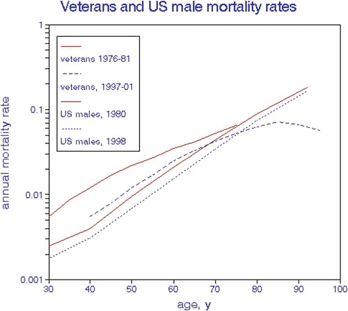
We assessed the overall health status of the cohort in terms of annual mortality rates. shows that the exponential increase in age-specific rates of the cohort slowed over time and with age, presumably because of depletion of the most vulnerable cohort members. At age 50, the veterans’ risks were about twice the national average for U.S. males, but this difference disappeared by about age 75 ().
Figure 1. Trends in veterans’ and U.S. male mortality rates.
Measures of ambient air quality
We used data from EPA regulatory monitoring sites and from the Inhalable Particulate Network (IPN) (Watson, Chow, and Shah Citation1981), as assigned to counties. All of the particulate measures were based on annual mean 24-hr averages, as were NO2 and the modeled estimates. Because of their typical diurnal and spatial variability and thus possible acute responses, we used the mean annual 95th percentiles for ozone (O3), carbon monoxide (CO), and SO2, designated as “peak” values.
We evaluated all of the criteria pollutants in addition to 19 constituents of PM2.5 and 12 “hazardous” pollutants (HAPs) (). These analyses were necessarily limited to counties having air quality monitoring stations, and for some pollutants this incomplete coverage limited the numbers of subjects included in the regression models. Routine ambient air quality monitoring data were obtained back to the early 1970s. Size-classified particulate matter data from 1979–1983 were obtained from the Inhalable Particulate Network (IPN), and from EPA’s Speciation Trends Network (STN) for fine particle constituents in 2002.
Table 2. Mean values of air quality and traffic variables.
Atmospheric modeling by Atmospheric and Environmental Research, Inc. (AER), was used to attain nationwide coverage for SO2, SO42−, O3, and elemental carbon (EC). County-level emission densities were used to estimate HAP concentrations. Use of nationwide data enlarged the operational data set and eliminated any biases due to nonrandom placement of ambient air quality monitors. shows reasonable agreement among data sources for selected pollutants, including modeled estimates. Note that “diesel PM” was defined by EPA and may include various other particles in addition to EC.
Table 3. Mean concentrations by data source.
The more recent Veterans Cohort papers (Lipfert et al. Citation2006a, Citation2006b, Citation2008, Citation2009) featured vehicular traffic density as a marker for mobile source pollutants, including tailpipe exhaust, noise, odors, tire and brake dust, lower socioeconomic status, and/or driving stress. Vehicular traffic data were obtained as county-level annual vehicle-mile traveled (VMT) for 1985, 1990, and 1997; we then normalized by dividing by county land area and converted to metric units (VKTA). We had independent VKT data for both gasoline- and diesel-powered vehicles that were highly correlated; we used the former in all regressions. Using county-level data for this purpose assumes homogeneity within a county; we thus assume that any local exposure differences in embedded highway configurations will average out. However, the county-average VKT and HAP data basically describe places and not necessarily the exposures of their inhabitants, who likely do not remain in their domicile and neighborhoods and spend most of their time indoors where air quality can be very different (Lipfert Citation2015). Other studies have focused directly on places such as proximity to vehicular traffic or “green” spaces (Vienneau et al. Citation2017; Villeneuve et al. Citation2012). Residential mobility could also be an issue; here we assume that subjects remain in the same county during follow-up, which is a reasonable assumption for this age group.
Statistical analysis
The Washington University proportional hazards regression model (Lipfert et al. Citation2000) included the following personal characteristics: smoking status (ever, current), race indicator, and height, as linear relationships. Age, systolic and diastolic blood pressures, body mass index (BMI) were represented as nonlinear relationships by using separate variables according to quintiles or deciles. All of this information was based on conditions at recruitment.
In addition to county-level ambient air quality measures, we added additional contextual variables on education, fraction living below the poverty level, climate, and fraction of African Americans as nonlinear relationships, in six levels. Thirty-eight independent variables were used in single-pollutant regressions. Our basic goal was to model the various factors influencing mortality rather than to simply “control” for them. Typically, 18 of the nonpollution variables were statistically significant in a given model run.
We selected annual heating degree-days as a measure of climate that could affect mortality in any of several ways: heat/cold stress, fraction of time spent outdoors, effects of indoor air pollution, regional lifestyle, or ethnicity. This variable has been used in several other studies of health effects (Lipfert Citation1980a, Citation1980b; Lipfert et al. Citation1988; Lipfert and Morris Citation2002)
Initially, we ran proportional hazards models of all-cause mortality for three follow-up periods: 1976–1981, 1982–1988, and 1988–1996. Deaths up to 2001 were subsequently added to the database, providing a fourth mortality period, 1997–2001. Most of the analyses were done for each period separately in addition to the overall periods (1976–1996, 1976–2001). The mean birth year was about 1925; mean attained ages were thus 58, 65, 70, and 80 yr in the four follow-up periods, respectively. Most of these veterans would have served during World War II.
Quantifying risks
We expressed mortality risk coefficients in various ways in our published papers. The current literature favors the use of arbitrary fixed concentration increments, i.e., 10 μg/m3 or 10 ppb, for various pollutants. This may be convenient for pollution abatement analysis but can be misleading when applied to pollutants of fundamentally different scales such as PM2.5 versus PM10 versus EC versus O3. Here we use the econometric concept “elasticity,” defined as percent output/percent input or (change in output/mean output)/(change in input/mean input). In proportional hazards analysis, regression coefficients are given in fractions per unit of input (%/100), which is equivalent to ln(RR). Multiplying by the mean input value yields the elasticity, which we denote as “mean effect” in this paper. This metric imparts similar risk implications to pollutants of any scale, from ng to mg to ppb to ppm. Relative risk (RR) is computed as exp(mean effect). When an independent variable is expressed as a logarithm, the proportional hazards regression coefficient equals the elasticity.
We used a slightly modified procedure to express risks associated with peak O3, which tends to have different frequency distributions from other pollutants in that the minimum values tend to be substantial fraction of the mean. Accordingly, we used the difference between mean and minimum concentrations.
To save space in the tables, we indicate statistical significant risk estimates with bold face rather than with confidence intervals. This is consistent with our basic intent to describe our findings rather than test hypotheses. Confidence intervals (CIs) are based on 95th percentiles.
Results
We begin by summarizing and reinterpreting findings from the six published papers, primarily for coherence, and focusing on relative timing of exposure. We then consider relationships with temporal trends. summarizes the entire suite of results of statistical significance (positive, (negative), none) in conjunction with the mean pollution values. Associations with NO2 and peak O3 remained significant as air quality improved over time. Traffic density remained significant during the period of reducing tailpipe emissions. Results for the various PM measures were mixed; only 4 of the 12 STN associations were significant. By contrast, all but 1 of the 19 modeled measures with nationwide distributions were significant, even as limited to the 1997–2001 mortality period. shows consistency among mean values of pollutants as obtained from different sources, including modeling.
Exposure timing
These veterans were followed from 1976 to 2001; we reported their survival in four sequential subperiods. Ambient air quality improved substantially during this period (), thus allowing longitudinal gradients to be considered as well as the traditional spatial patterns. It is important to recognize that an “adverse effect” is traditionally defined as response to change such as surgery, new medication, or periodic smog episodes that imply timing (Sherwin Citation1983), as opposed to the characterization of spatial gradients per se. In a purely spatial analysis, change would imply residential relocation or perhaps moving to a new hospital.
Timing of exposure with respect to (significant) response can have important implications with respect to establishing causality:
Response before exposure: spurious association.
Response independent of exposure timing: associations with residential locations (including indoor air quality) rather than with dynamic outdoor exposures.
Response coincident with exposure followed by decreases: acute effects.
Delayed response (lagged): latency period for initiating chronic disease.
Response increasing with lag and duration of exposure: development of chronic disease.
We found evidence for items 1–3 but not 4 or 5. Some of our air quality measures were limited to a single exposure period, thus precluding examinations of response dynamics. Exposure issues are discussed further under ‘Concluding discussion’ below.
Previous findings
presents matrices of risk estimates for total suspended particulate (TSP)/PM10, SO42−, PM2.5, NO2/NOx, peak O3, and traffic density by exposure and mortality periods as obtained from our prior publications. Risks in based on modeled nationwide exposures were limited to counties with either high traffic density or NO2 monitoring data. The early PM2.5 data were obtained from the Inhalable Particulate Network (IPN), which had fewer monitoring sites located near VA clinics. The 70 estimated relative risks in range from a 25% benefit to 20% excess risk. Means and confidence intervals of the columns are shown in the bottom row. The mean risks and confidence intervals by pollutant are 1.004 (0.96–1.05) for all PM, 1.059 (1.01–1.11) for NO2, 1.044 (0.94–1.16) for peak O3, and 1.049 (1.04–1.06) for traffic density. Eighteen of the 70 estimates in were statistically significant (shown in boldface), notably traffic density and peak O3; the two PM2.5 estimates were significantly negative (RR < 1.0). Risks for the entire follow-up period for each exposure period are shown in the right-most column; 4 of the 23 estimates were significant. PM2.5 was only statistically significant (positive) with 1989–1996 mortality in 1 of 11 estimates and was never significant (positive) in combination with other variables.
Table 4. Relative mortality risks for counties with ambient air quality monitors.
Except for PM2.5, there are only minor differences among the column means in ; the largest estimates are for NO2/NOx, peak O3, and traffic density. The NO2/NOx risks show no trends, and the subperiod risks tend to exceed their whole-period counterparts. Except for the 1997–2001 entries, there are only minor differences across mortality periods, despite aging of the cohort. Risks for the entire period tend to increase with exposure year, as do risks along the matrix diagonals. Relative risks range from 1.026 to 1.247 in the most recent mortality and exposure periods; only the traffic-density risk estimate is statistically significant, in part because of the larger sample size.
None of the of the published Veterans Cohort papers considered indoor air pollution exposures, which can be important given the large fraction of time typically spent indoors (Lipfert Citation2015). Substituting outdoor for personal exposure introduces substantial measurement error that is difficult to quantify and may bias risk estimates. PM and NO2 have appreciable indoor sources that can increase personal exposures (Li et al. Citation2006; Neas et al. Citation1991). Ozone and SO2 are adsorbed onto indoor surfaces, thus reducing personal exposures. Traffic-related pollutants are unlikely to have residential indoor sources and are characteristic of places rather than human exposures per se. Okokon, Taimisto, and Turunen et al. (Citation2017) showed that traffic noise is strongly correlated with in-vehicle EC and ultrafine PM but not PM2.5.
Discussion
Interpretation
We are interested in the trends shown in in addition to statistical significance. We used ordinary least squares (OLS) regressions across both mortality and exposure periods in meta-analyses to examine the dependence of these risk estimates on particle size, mortality year, lag between exposure and response, and use of the overall follow-up period (mortality from 1976 onward). Mortality year was never a significant predictor in these OLS regressions, nor was particle size. The most consistent finding was a negative effect of lag, suggesting relatively prompt rather than cumulative responses (). These lag effects showed risks decreasing by 0.004–0.007 per year, suggesting that mortality effects did not persist more than 5–10 yr after exposure. Lag effects were not seen in the NO2 data, nor were effects of exposure duration.
Table 5. Summary of lag effects.
NO2 risk estimates were not significantly associated with any independent variable and had the smallest regression error (SEE). Traffic density risks did not vary by mortality year.
Since these risk estimates are based on mean concentrations, we would expect them to decrease as air quality improved over time. Failure to do so suggests that the estimated risks may actually be associated with (presumably invariant) residential locations per se, of which relative traffic density is an example. We found no evidence that improved outdoor ambient air quality reduced mortality risks in this cohort.
Below we present new analyses of the Veterans Cohort data intended to distinguish between the effects of aging and other secular trends.
Findings from other cohorts
Quantifying long-term public health benefits of air pollution abatement requires identifying contributions of acute and previous long-term exposures; here we briefly consider what other investigators have reported. Laden et al. (Citation2006) published a thorough analysis of 8 yr of additional follow-up of the Harvard Six Cities Study. They remarked that the relevant PM2.5 exposure period could be a short as 1 yr and that decades of exposure may not be required to develop risks they described as “chronic.” They also showed that city-specific mortality risks for the additional 1990–1998 follow-up period were essentially nil. Lepeule et al. (Citation2012) extended the Six Cities follow-up to 2009 for a total of 35 yr, one of the longest in the literature, and considered time-varying effects of smoking, sex, and education in conjunction with PM2.5. They considered four subperiods, of which only 1983–1991 (mean age = 63 yr) produced a statistically significant risk. They based their PM2.5 estimates on data from 1974–2009, thus permitting cumulative exposures to be considered, as had been suggested by Dockery et al. (Citation1993). Their results showed the best model fit (lowest Akaike information criterion [AIC]) for 1-yr moving average exposures, although there were only small differences over the range 1–5 yr. Only 18 yr of follow-up (to a mean age of 74 yr) have been considered with the American Cancer Society cohort (Krewski et al., Citation2009), and most other cohorts have been followed for shorter periods.
Most studies of long-term effects of ozone have been based on annual averages, with mixed results (Atkinson et al. Citation2016) However, Jerrett et al. (Citation2009) used daily maximum levels in conjunction with mean PM2.5 with the American Cancer Society cohort; significant O3 effects were only found for respiratory mortality, and O3 had a significant negative association with all-cause mortality.
Conclusion from previous Veterans Cohort publications
The maximum statistically significant mortality risks for the pollutants in range from 1.06 to 1.19 (mean = 1.13) and are most consistent for traffic density. This pollutant indicator is also the least likely to be influenced by indoor air pollution sources. Risks associated with NO2 and traffic density did not vary with follow-up subperiod. However, traffic density fundamentally represents the characteristics of a place, i.e., county, for which relative rankings may have been more or less invariant during follow-up. We find no evidence that long-term mortality risks in this cohort decreased as air quality improved over 25 yr. However, although air quality improved, the cohort aged; the results of do not permit distinguishing between these trends, which is the object of the following section as follows.
Age-specific mortality risks and trends
The Cox proportional hazards model may be represented as follows:
where the β values are assumed to remain constant and to apply to all subjects regardless of age, race, year of death, or geographic location. By and large, these assumptions have not been tested. Here we use parametric analyses to examine differences by subject age and year of death that cannot be separated in conventional cohort studies. For example, risks declining with extended follow-up could be due to improved air quality, aging of the cohort, or changes in confounders such as reduced smoking or improved medical care. Increasing risks over time could result from accumulated effects of continued exposure.
Objectives, methods, and data
We discuss several questions with respect to risks of air pollution exposures and to important covariates such as smoking or climate:
How do mortality risks vary with age?
How have these age group risks changed over time?
Have confounders changed over time?
What are the implications for air pollution model development and dose-response functions?
Cohort studies differ from population studies in that the composition of the cohort changes over time as the cohort ages and the most vulnerable subjects are lost. By contrast, population-based age groups such as Medicare are continually augmented with new subjects. Effects of aging may be confounded by other temporal trends such as better air quality, improvements in medical care, or reduced smoking. Our purpose here is to examine relationships among β values by applying eq 1 to subsets of the cohort defined by age decile and by mortality follow-up period. We established age deciles and examined them separately for each of the four follow-up periods (n = 40) and for the total period (n = 10). This protocol greatly reduced sample sizes and introduced additional random noise. Accordingly, we used averaging and OLS regression methods to examine trends in the sets of β values.
Analyzing variability among regression coefficients across the 40 model runs allowed us to examine pollution risk coefficients in addition to the model regression coefficients that had not been examined elsewhere. Risks associated with confounders have seldom been reported in air pollution studies. We then consider whether the putative control for a covariate is consistent with what has already been established from nonpollution studies. Effects of smoking are seldom reported separately in air pollution studies and are thus a prime example.
We regressed β values for selected independent variables against polynomial functions of age and with a linear function of time to explore relationships with both subject age and year of death. We then selected the age function producing the best overall fit and displayed the trends in –. We included the raw data points where feasible.
Figure 2. Effects of current smoking status on mortality risk, based on proportional hazards regression coefficients by age group and time period.
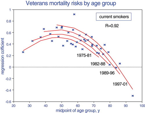
Figure 3. Effects of current smoking status on mortality risk, based on proportional hazards regression coefficients by age group and time period, showing average years of birth.
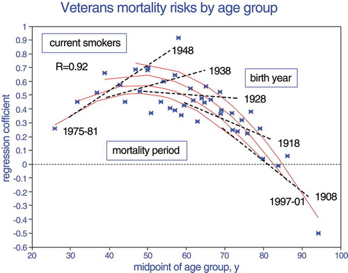
Figure 4. Effects of current smoking status on mortality risk, based on proportional hazards regression coefficients by age group, time period, and birth year.
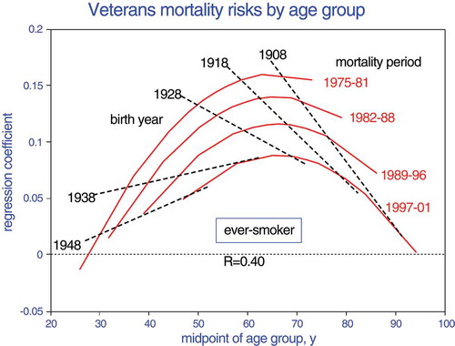
Figure 5. Effect of living in poverty on mortality risk, based on proportional hazards regression coefficients by age group.
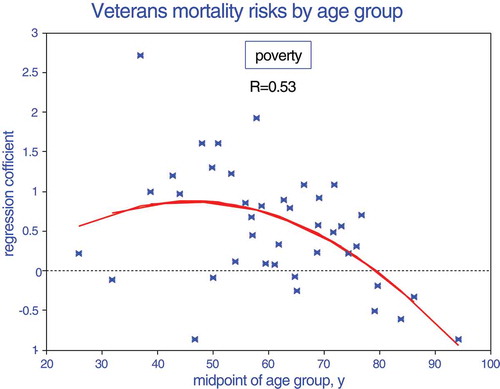
Figure 6. Effect of county space heating degree-days, based on proportional hazards regression coefficients by age group and time period.
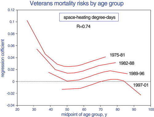
Figure 7. Average mean effects of traffic density by age at recruitment, less minimum and maximum estimates.
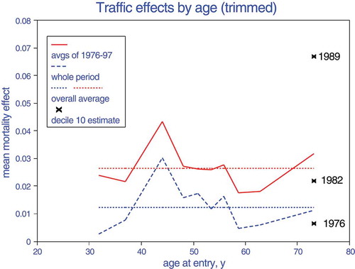
Figure 8. Average mean effects of benzene by age at recruitment, less minimum and maximum estimates.
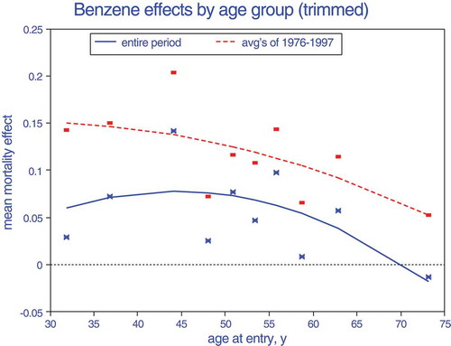
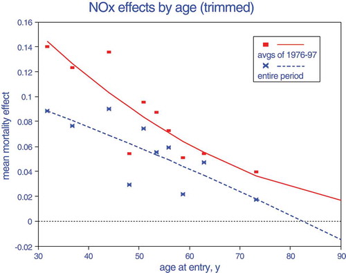
Figure 9. Effect of exposure to nitrogen oxides on proportional hazards mortality regression coefficients.
The independent variables we selected comprise three groups:
Lifetime exposures whose intensities have decreased over time such as air pollution and perhaps smoking.
Personal characteristics that may have remained essentially constant: race, education, height, characterization of residential location (i.e., poverty status).
Climate effects that have either remained constant such as geography or those that have changed such as cleaner space-heating fuels and increased use of residential air conditioning.
We selected three pollutants with nationwide distributions for these analyses: a criteria pollutant (NOx), a hazardous species (benzene), and a geographic descriptor (traffic density). We used 2002 air quality data for each period, the only year for which we had nationwide estimates. We opted for nationwide coverage instead of temporal detail in order to preclude bias from partial monitoring coverage, in contrast to the previous analyses of exposure timing.
Results
presents mean values by age decile for the three pollutants. For each follow-up period, we augmented the mean age values by the elapsed time between periods; for example, the mean age for the 10th decile was 73 at recruitment in 1976. Thus, 23 yr later in 1999 it would have nominally been 96, based on consistent age distributions.
Table 6. Mean pollutant values by age decile.
Mean values for the three pollutants decreased with age by 7–13% and standard deviations increased. Traffic density (ln[VKTA]) was the most variable of the three pollutants (coefficient of variation [CV] = 1); benzene was the least variable (CV = 0.4). CVs increased by about 29% over the age range, which could have resulted in a greater likelihood of statistical significance for the elderly. [Lipfert and Wyzga (Citation1997) showed that increased natural variability of an independent variable (excluding measurement error) increases the t value, ceteris paribus.] Although the total number of cohort subjects decreased about 34% during the mortality follow-up period, the 10th decile decreased by 90%. This is an important difference with respect to population-based studies, which are not constrained by cohort membership.
shows how mortality risks varied with time for the four subperiods compared with the total follow-up period. The risks of current smoking status are roughly an order of magnitude larger than those for the pollutants based on mean concentrations. Risks associated with smoking, traffic density, or benzene were steady over time, but NOx risks decreased, as shown for NO2 in . The 1976–2001 risk estimates compare reasonably well with averages over the four separate periods for smoking but not for air pollution, for which the separate analyses roughly doubled the estimated risks. This suggests that effects of confounding variables changed over time such that during follow-up, employing smaller time steps improved the overall model fits. The whole-period analyses thus underestimated the risks associated with air pollution.
Table 7. Summary of mean risks (ln[RR]) by follow-up period.
Trends in age-dependent risks are displayed in –. Age-specific mortality risks for smokers (–) are complex, but the age polynomials fit the data exceptionally well. For current smokers, risks increase with age until about age 50 when the relative risk is about 2.0 and then decrease rapidly, presumably due to selective depletion of the cohort. Smokers who survive will have demonstrated robustness and thus decreased risk. The effects of time (mortality period) may relate to year of birth (). Those born in ~1948 and died at age 50 in ~1998 will have consumed more pack-years than those who died at age 30 in ~1978 and are thus at greater risk. By contrast, those born in 1928 and survived until 1998 must have been basically more robust in spite of their additional pack-years of exposure. Those born in 1908 will have already survived even more pack-years by the time of recruitment (1976) and continue to outlive those born later. These trends are limited to closed cohorts that experience depletion of the most susceptible subjects over time, as shown in .
Ever but not current smokers (i.e., quitters) show similar trends with age but opposite trends with mortality period (). Maximum risks are only about 20% of those for current smokers and occur later, at age 60. This trend may reflect partial reversibility of smoking damage. Risks increase for earlier birth cohorts, presumably because they had experienced more pack-years before quitting. Overall, – show increased risks from longer cumulative exposures followed by decreased risks due to cohort depletion, which would not be seen in a population study.
The risks of living in a poverty area () are insensitive to time or exposure period and are similar to those of continued smoking. Poverty risks decrease after about age 50, presumably also because of cohort depletion.
Risks associated with heating degree-days () could represent exposure to domestic heating emissions, sensitivity to hot or cold weather, or a marker for latitude or regional gradients. Risks were initially greater in northern climates and strongly attenuated over time and with age, reducing the relative risks for the elderly of having lived in colder regions. This relationship could also suggest trends toward cleaner space-heating fuels or better-insulated housing.
Our estimated age relationships with race, education, and height were linear and are not depicted graphically. Risks associated with race declined over time. The effect of education on mortality risk was not significant based on separate follow-up periods (n = 40) but was significantly positive for the entire period (n = 10). The advantage of education was attenuated with age. We found that longevity decreased with increased height (stature). All of these findings contribute to understanding the dynamics of health effects.
Relationships with air pollution were more complex and are shown in –. Because these data are quite noisy, we averaged the estimates over the four subperiods for each decile. For this process, we did not consider the two extremes (decile 1 for 1976–1981, decile 10 for 1997–2001), i.e., we “trimmed” the data set. All three pollutants show maximum risks at middle and younger ages, with a sharp decline thereafter, roughly consistent with all of the other relationships. An exception is seen for traffic density at maximum age: risks increased sharply over time as the group aged (maximum group = 94). Current smoking () shows similar age-risk relationships across the four subperiods, and the peak risks are similar to what was reported by the U.S. Public Health Service (Citation1964).
We fit quadratic relationships to the benzene and NOx group averages; the traffic density relationship appears to be cubic because of the elderly upturn, but having only 10 data points precludes curve-fitting. We contrast these age relationships between the averages over the subperiods and the estimates over the entire period. For traffic density and benzene, the risk is approximately doubled; for NOx, the subperiod averages are about 50% greater. For comparison with , it is important to note that about half of the cohort was aged 45–55 at recruitment, ages at which mortality risks of some pollutants are maximized.
summarizes the relationships seen in –. The correlation coefficients (R2) indicate how well these polynomial models fit the output of the proportional hazards models, ranging from extremely well for current smoking status to nonsignificantly for education. The maximum or minimum relative risks in the table reflect the extremes of each curve fit. The risk for current smoking is consistent with values from the 1964 Surgeon General’s Report, and the risk of living in a poor neighborhood is just as strong.
Table 8. Summary of relationships with mortality.
Discussion
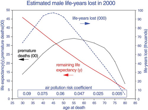
The extant literature reports statistically significant mortality relationships with various air pollutants. Our analysis is intended to examine the detailed support for such findings and to place the risk relationships into perspective. They represent percentage changes to baseline mortality rates that increase exponentially with age (). The numbers of pollution-related deaths may thus increase with age even if risk coefficients do not. As an illustration, we used vital statistics for U.S. males from 2000 to estimate the numbers of premature deaths and losses of life expectancy that would result from the age-dependent risk function of (Minino et al. Citation2002; Wei et al. Citation2012). shows that whereas the mortality risk coefficients peak at age 30, the number of premature deaths peaks at age 55 and the number of life-years lost (change in life expectancy times the number of premature deaths) peaks at age 45. The larger risk coefficients before about age 40 are thus less crucial. For comparison, the age-weighted NOx risk coefficient is 0.032, which is similar to the all-age estimate for traffic density.
Figure 10. Example of potential public health importance of age-related air pollution risks based on vital statistics for U.S. males in 2000. Life-years lost are expressed in thousands; premature deaths, in hundreds.
Only risks associated with smoking and heating degree-days showed temporal gradients after age adjustment. Smoking trends reflect cumulative exposures (pack-years) up to middle ages, with cohort depletion effects after about age 60. Smokers born before 1928 who remained in this cohort must thus have enjoyed exceptional survivability (). Effects of climate/space heating were strongly attenuated over time (). Lepeule et al. (Citation2012) found maximum mortality risks for the Harvard Six Cities at about age 63.
The absence of time dependence in this analysis and in indicates that mortality risks associated with air pollution are the same at a given age regardless of follow-up year or age at entry. Age is the only other time-dependent variable, and the analysis indicates that other temporal changes such as in medical care or subject susceptibility did not materially affect these pollution risk estimates. We did not consider interactions between age and time. Selective depletion during aging is seen with all variables except heating degree-days and traffic density, which are characteristics of locations rather than individuals.
Conclusions from age-specific analyses
We conclude that the basic structure of the WUSTL proportional hazards model is supported by independent mortality relationships with nonpollutant variables as functions of age, especially for smoking. Mortality relationships with smoking and poverty are an order of magnitude stronger than those with air pollution and are thus critical for valid risk estimates. We show that effects of confounding variables change during the life of a cohort. Associations of air pollution with mortality also change with age; comparisons of cohort studies are thus sensitive to the ages of members during follow-up.
Concluding discussion
Findings from our six published papers (Lipfert et al. Citation2006a, Citation2006b, Citation2000, Citation2003, Citation2008, Citation2009) were originally presented in various formats. We clarified those presentations and recast the results as relative risks, similarly with other cohort analyses. Our research has primarily been concerned with identifying consistent associations, the subpopulations most at risk, and the implications for public health. presents issues and responses that developed during the project and represents a synthesis of our overall findings.
Table 9. Summary of findings.
We made extensive use of subset analyses, a protocol that has seldom been used with other cohorts. Stratification by follow-up period showed that responses were most consistently associated with concurrent exposures. Stratified analyses showed greater risks in more urban areas and in those with ambient air quality monitors. Stratification by subject age showed that risks associated with pollutants and with confounders varied by age; risk coefficients for benzene and NOx decreased and showed minimal risks above about age 70. These trends may have resulted from continuing depletion of the cohort of its most susceptible members.
During the 25-yr follow-up, the acceleration of veterans’ mortality rates slowed () and air pollution levels were approximately halved (). However, definitions and measurement methods for PM evolved during this period, precluding valid trend analyses. For the country as a whole, vehicle-miles driven doubled but fuel use increased by only about 40%, population density increased about 30%, the poverty rate stayed roughly constant, prevalence of obesity doubled, national cardiovascular death rates were halved, and cancer incidence increased by 20%. It is thus clear that a dynamic approach to follow-up is needed.
Coherence of risk estimates
We grouped the air pollutants in this study as follows: traffic-related pollutants, particulate species, peak ozone, and various hazardous pollutants. summarizes our risk estimates based on air quality data from several different sources: (1) routine EPA monitoring, (2) the EPA STN database, (3) traffic count data, (4) nationwide dispersion modeling, (5) emission rates of hazardous pollutants, and (6) the Inhalable Particulate Network (IPN).
Table 10. Coherence of relative risk estimates (as elasticities) based on various data sets and follow-up periods for all ages.
The traffic-related risk estimates are quite coherent given the variety of databases that were used. The mean traffic-related mortality risk is 1.10; complete elimination of traffic effects could thus reduce mortality by 10%, but a realistic pollution abatement program might save only 2–3%. Note that the more specific pollutants, EC and NOx, appear to pose greater risks and that the estimated risks associated with NO2 and traffic density were essentially invariant over time, as shown in .
Risk estimates for particulate matter are not coherent and (counterintuitively) indicate greater risks for larger particles. The largest estimates were for PM10, corresponding to 1.045 per 10 μg/m3, similar to other studies (Fischer et al. Citation2015; Medina et al. Citation2004).
The ozone data were obtained from EPA monitors; risks associated with peak ozone were based on mean − minimum concentrations. These risk estimates are also coherent, but only three are statistically significant. A reasonable estimate of the overall O3 mean effect is given by the average, 1.075 (1.03–1.11), corresponding to 1.024 per 10 ppb. We also estimated the risk for mean rather than peak O3 with the STN data set and found a nonsignificant relative risk of 0.82, thus justifying our use of the peak measure. Note from that there is no trend toward reduced risks with cleaner air (later periods). Relative risks from joint regressions with O3 and traffic-related pollutants based on mean − minimum concentrations without lag include peak O3 (1.091) with EC (1.115) and 1.215 for the sum, and peak O3 (1.023) with traffic density (1.080) and 1.105 for the sum.
As indicated in , the O3 risk estimates show significant lag effects, suggesting that acute mechanisms might be involved, especially with peak concentrations. Since short-term effects are included in long-term effects, it is possible that both effects may be operating in a cohort study (Medina et al. Citation2004).
Estimated relative risks for the hazardous pollutants ranged from 0.98 to 1.20, with a mean of 1.052 (1.01–1.09). No temporal trend information was available for these pollutants. This considerable range in risk estimates indicates the need for further study and more complete databases.
Artifact versus reality
Given the large number of significant risk estimates of similar magnitude, other considerations are required to derive valid conclusions. These include copollutant confounding and interpretation of exposure estimates.
Copollutant effects
summarizes 2-pollutant regression results from the various published studies; correlation coefficients are also shown for each combination. Traffic density remained significant in each case except in combination with EC, which is associated with traffic, as are nitrogen oxides. Peak O3 was significant with EC in a 2-pollutant model, thus providing an example of regional and local effects combined (note the weak correlation).
Table 11. Statistical significance and correlations (in parentheses) in 2-pollutant models.
Exposure considerations
Exposure estimation is perhaps the weakest link in air pollution epidemiology, and random errors can attenuate risk coefficients. With measured concentrations, uncertainties can result from local pollution sources and monitor placement and with spatial extrapolation. Indirect measurements from satellites also entail uncertainties, as do various types of modeled exposures. Land-use modeling and dispersion models based on emissions depend on adequate validation. The validity of temporal mismatching is contingent upon strong correlations over time and absence of either new emission sources or pollution control programs. However, uncertainties resulting from lack of personal exposure and dose information (discussed below) are likely to dominate.
Risk estimates are intended to link exposures with outcomes, here long-term mortality risks. Abatement of outcome requires modification of exposure and hence dose to target organs and is thus contingent upon the validity of the implied exposure metrics. In the Veterans Cohort study, we considered two distinct types of exposure estimates:
Annual average concentrations of specific pollutants as surrogates for personal exposures that are not available in studies of this type, especially for lengthy periods of follow-up. Further, these unavailable personal exposures are themselves surrogates for doses to target organs. Note that the observed outcomes in a cohort study are attributed to individuals rather than to the spatial confines of the monitoring network from which individual exposures were imputed, thus creating a potential mismatch between (average) exposure and (individual) outcome. This paradigm assumes that reducing the pollutant concentration at a central monitor will reduce doses to target organs of all individuals within the defined spatial monitoring confine. The relative extent of such confines (cities vs. counties vs. metropolitan areas) directly affects the degree of measurement error involved in this assumption.
Characteristics of the places, i.e., spatial confines, in which the cohort members resided at recruitment. These characteristics include ambient air quality but also geographic features such as green space or highways, or air pollution sources whose emissions may not be observed by the ambient monitoring network. In a spatial analysis, all “contextual” variables fundamentally relate to places rather than individuals, and numerous studies have shown their importance (Jerrett et al. Citation2005; Lipfert et al. Citation2000; Willis et al. Citation2003). This modality also assumes that these spatial characteristics apply to all cohort members who resided in this place at recruitment. (Relevant nonuniform spatial factors include the characteristics of residential housing stock that affect indoor air quality, indoor air pollution sources, and the rate of penetration of outdoor air pollution.) With this exposure model, mortality risks are nonspecific and imply that living in a given place is riskier than in another, for all residents. Those risks are linked to the parameters used in the analysis, such as population density, ethnic splits, climate, income inequality, and traffic density. Pollutant dose per se is not involved. In this paradigm, abatement must be achieved by modifying the descriptive characteristics of the area or by moving to a cleaner area and benefits can only be realized by moving to a cleaner residential location (Wu et al. Citation2013, Citation2014). By contrast, benefits of cleaner air depend on temporal changes, notably emission reductions.
Indoor air quality can only be characterized for individual residences and lifestyles; the determining factors and personal exposures for individual cohort members are thus unknown, resulting in substantial measurement error and biased risk estimates. Given this fundamental limitation, (outdoor) ambient air quality must be considered a characteristic of place rather than an estimate of individual personal exposure.
Implications for study design
The classic long-term cohort study protocol is based on the characteristics of individuals, tracking their progress over time and accounting for changes during follow-up such as smoking or BMI. The basic model is thus essentially temporal, in keeping with the concept that an “adverse effect” requires a change such as tumor development, heart attack, or stroke (Sherwin Citation1983). Here, subject aging and improved air quality represent changes affecting outcomes.
However as a practical matter, in order to obtain a sufficiently large cohort, range of exposures, and regional diversity, long-term air pollution studies have become essentially spatial, i.e., cross-sectional. In such purely spatial (cross-sectional) studies, “change” would require residential relocation (Wu et al. Citation2013, Citation2014).
Spatial designs involve scales that must be extensive enough to provide a sufficient range in long-term ambient air quality concentrations. Since personal exposure information is never available for enough subjects or sufficiently long periods, it is necessary to assume that point measurements of ambient air quality represent personal exposures of individuals. At this point, a cohort study becomes “ecological” and the distinction with population studies is blurred. Such studies then focus on the places that have the required air quality data, and this requires attention to other characteristics of those places that may influence health outcomes, hence the need for “contextual” covariates discussed above.
Statistical power is based on the number of events, the numbers of subjects in each, and the length of follow-up time. Large studies are required to detect the typically weak associations with air pollution. Since it is more practical to extend follow-up time than to recruit additional subjects, temporal trends during follow-up can be important. Twenty-year follow-up periods involving aging of the cohort and improved ambient air quality are not uncommon. Studies intended to be primarily spatial are thus inexorably also temporal (Medina et al. Citation2004). Risk analysis must distinguish between aging, which can involve increased susceptibility and loss of the most vulnerable subjects, improved air quality, and other temporal trends such as population growth and better medical care. This is not possible if the entire follow-up period is considered in toto and temporal trends are obscured. Conventional long-term studies have been based on the premise that the target relationships are independent of subject age and of temporal changes in exposure and covariates. We showed that this is not the case by considering four sequential subperiods of follow-up.
Given the cost and time required to extend monitoring networks, some type of ambient air quality modeling may be required. Unlike measured pollutants, the lower ranges of modeled exposures are not limited by minimum detectable levels and these greater ranges likely played a role in achieving statistical significance in the Veterans Cohort study. The traffic density variable has a range of 4 orders of magnitude across the entire country and 2.5 orders for counties with air quality monitors, whereas monitored air quality ranges over only 1–2 orders of magnitude. The uncertainties of exposure modeling will always be less important than those created by the absence of personal exposure data.
Overall conclusion
Our analyses of subsets of the Veterans Cohort confirm the basic structure of the WUSTL proportional hazards model and find statistically significant long-term associations of all-cause mortality with many pollutants. We find that the most consistent and plausible long-term risks are associated with vehicular traffic pollutants. Our results for peak O3 suggest shorter-term responses. We found significant risks associated with a wide range of hazardous air pollutants but not consistently with particulate matter.
Our new results show that mortality risks tend to peak in middle age and are minimal for the very elderly; more attention should thus be given to ages <60 and >75. Our analyses of age-specific regression coefficients allowed detailed examination of the behavior of confounding variables; our estimates of smoking effects are consistent with public health reports, and we found that neighborhood poverty status was equally important.
We found that after controlling for aging, mortality associations with traffic-related pollutants were invariant over time during this period of implementation of tailpipe emission controls. This suggests that those risks are associated with heavy traffic locations per se rather than the decreasing pollution exposures during follow-up. Thus, we found no evidence that cleaner air reduced mortality in this cohort. Given the specificity and timing of the Veterans Cohort, we do not expect these results to be definitive, but we hope that the methods we introduced here will be instructive for future epidemiology studies.
Acknowledgment
All of the proportional hazards modeling for this project was performed by Jack Baty of WUSTL, including those in the unpublished work.
Additional information
Funding
Notes on contributors
Frederick W. Lipfert
Frederick W. Lipfert is an independent consultant based in Greenport, New York.
Ronald E. Wyzga
Ronald E. Wyzga is a senior technical executive at the Electric Power Research Institute in Palo Alto, California.
References
- Atkinson, R. W., B. K. Butland, C. Dimitroulopoulou, M. R. Heal, J. R. Stedman, N. Carslaw, D. Jarvis, C. Heaviside, S. Vardoulakis, H. Walton, and H. R. Anderson. 2016. Long-term exposure to ambient ozone and mortality: A quantitative systematic review and meta-analysis of evidence from cohort studies. BMJ Open. 6 (2):e009493. doi:10.1136/bmjopen-2015-009493.
- Dockery, D. W., C. A. Pope 3rd, X. Xu, J. D. Spengler, J. H. Ware, M. E. Fay, B. G. Ferris Jr, and F. E. Speizer. 1993. An association between air pollution and mortality in six U.S. cities. N. Engl. J. Med. 329 (24):1753–1759.
- Dockery, D. W., F. E. Speizer, D. O. Stram, J. H. Ware, J. D. Spengler, and B. G. Ferris Jr. 1989. Effects of inhalable particles on respiratory health of children. Am. Rev. Respir. Dis. 139 (3):587–594. doi:10.1164/ajrccm/139.3.587.
- Fischer, P. H., M. Marra, C. B. Ameling, G. Hoek, R. Beelen, K. De Hoogh, O. Breugelmans, H. Kruize, N. A. Janssen, and D. Houthuijs. 2015. Air pollution and mortality in seven million adults: The dutch environmental longitudinal study (DUELS). Environ Health Perspect. 123 (7):697–704.
- Jerrett, M., R. T. Burnett, C. A. Pope 3rd, K. Ito, G. Thurston, D. Krewski, Y. Shi, E. Calle, and M. Thun. 2009. Long-term ozone exposure and mortality. N. Engl. J. Med. 360 (11):1085–1095. doi:10.1056/NEJMoa0803894.
- Jerrett, M., R. T. Burnett, R. Ma, C. A. Pope 3rd, D. Krewski, K. B. Newbold, G. Thurston, Y. Shi, N. Finkelstein, E. E. Calle, and M. J. Thun. 2005. Spatial analysis of air pollution and mortality in Los Angeles. Epidemiology. 16 (6):727–736. doi:10.1097/01.ede.0000181630.15826.7d.
- Krewski, D., M. Jerrett, R. T. Burnett, R. Ma, E. Hughes, Y. Shi, M. C. Turner, C. A. Pope 3rd, G. Thurston, E. E. Calle, M. J. Thun, B. Beckerman, P. DeLuca, N. Finkelstein, K. Ito, D. K. Moore, K. B. Newbold, T. Ramsay, Z. Ross, H. Shin, and B. Tempalski. 2009. Extended follow-up and spatial analysis of the American Cancer Society study linking particulate air pollution and mortality. Res. Rep. Health Eff. Inst. 140:5–114.
- Laden, F., J. Schwartz, F. E. Speizer, and D. W. Dockery. 2006. Reduction in fine particulate air pollution and mortality: Extended follow-up of the Harvard Six Cities study. Am. J. Respir. Crit. Care Med. 173 (6):667–672. doi:10.1164/rccm.200503-443OC.
- Lepeule, J., F. Laden, D. Dockery, and J. Schwartz. 2012. Chronic exposure to fine particles and mortality: An extended follow-up of the Harvard Six Cities study from 1974 to 2009. Environ Health Perspect. 120 (7):965–970. doi:10.1289/ehp.1104660.
- Li, R., E. Weller, D. W. Dockery, L. M. Neas, and D. Spiegelman. 2006. Association of indoor nitrogen dioxide with respiratory symptoms in children: Application of measurement error correction techniques to utilize data from multiple surrogates. J. Expo. Sci. Environ. Epidemiol. 16 (4):342–350. doi:10.1038/sj.jes.7500468.
- Lipfert, F. W. 1980a. Statistical studies of mortality and air pollution: Multiple regression analyses by cause of death. Sci. Total Envir. 16:165–183. doi:10.1016/0048-9697(80)90022-4.
- Lipfert, F. W. 1980b. Statistical studies of mortality and air pollution: Multiple regression analysis stratified by age group. Sci. Total Envir. 16:103–122. doi:10.1016/0048-9697(80)90002-9.
- Lipfert, F. W. 2015. An assessment of air pollution exposure information for health studies. Atmosphere (Basel). 6:1736–1752. doi:10.3390/atmos6111736.
- Lipfert, F. W., H. M. Perry Jr, J. P. Miller, J. D. Baty, R. E. Wyzga, and S. E. Carmody. 2000. The Washington University-EPRI Veterans’ Cohort Mortality Study: Preliminary results. Inhal Toxicol. 12 (Suppl 4):41–73. doi:10.1080/713856640.
- Lipfert, F. W., H. M. Perry Jr, J. P. Miller, J. D. Baty, R. E. Wyzga, and S. E. Carmody. 2003. Air pollution, blood pressure, and their long-term associations with mortality. Inhal Toxicol. 15 (5):493–512. doi:10.1080/08958370304463.
- Lipfert, F. W., J. D. Baty, J. P. Miller, and R. E. Wyzga. 2006b. PM2.5 constituents and related air quality variables as predictors of survival in a cohort of U.S. military veterans. Inhal. Toxicol. 18 (9):645–657.
- Lipfert, F. W., and R. E. Wyzga. 1997. Air pollution and mortality: The implications of uncertainties in regression modeling and exposure measurement. J. AWMA. 47:517–523.
- Lipfert, F. W., R. E. Wyzga, J. D. Baty, and J. P. Miller. 2006a. Traffic density as a surrogate measure of environmental exposures in studies of air pollution health effects: Long-tern mortality in a cohort of U.S. military veterans. Atmos. Environ. 40:154–169. doi:10.1016/j.atmosenv.2005.09.027.
- Lipfert, F. W., R. E. Wyzga, J. D. Baty, and J. P. Miller. 2008. Vehicular traffic effects on survival within the Washington University-EPRI veterans cohort: New estimates and sensitivity studies. Inhal Toxicol. 20 (10):949–960. doi:10.1080/08958370701861512.
- Lipfert, F. W., R. E. Wyzga, J. D. Baty, and J. P. Miller. 2009. Air pollution and survival within he Washington University-EPRI veterans cohort: Risks based on modeled estimates of ambient levels of hazardous and criteria air pollutants. J. Air Waste Manag. Assoc. 59 (4):473–489. doi:10.3155/1047-3289.59.4.473.
- Lipfert, F. W., R. G. Malone, M. L. Daum, N. R. Mendell, and -C.-C. Yang. 1988. A statistical study of the macroepidemiology of air pollution and total mortality. Report BNL-52122, Brookhaven National Laboratory, April. doi:10.3168/jds.S0022-0302(88)79586-7
- Lipfert, F. W., and S. C. Morris. 2002. Temporal and spatial relations between age specific mortality and ambient air quality in the United States: Regression results for counties, 1960-97. Occup. Environ. Med. 59 (3):156–174. doi:10.1136/oem.59.3.156.
- Medina, S., A. Plasencia, F. Ballester, H. G. Mücke, and J. Schwartz. 2004. Apheis group. Apheis: Public health impact of PM10 in 19 European cities. J. Epidemiol. Community Health. 58 (10):831–836.
- Minino, A. M., E. Arias, K. D. Kochanek, S. L. Murphy, and B. L. Smith 2002. Deaths: Final Data for 2000. National vital statistics reports, 50 (15), Hyattsville, MD, National Center for Health Statistics. doi:10.1044/1059-0889(2002/er01)
- Neas, L. M., D. W. Dockery, J. H. Ware, J. D. Spengler, F. E. Speizer, and B. G. Ferris Jr. 1991. Association of indoor nitrogen dioxide with respiratory symptoms and pulmonary function in children. Am. J. Epidemiol. 134 (2):204–219. doi:10.1093/oxfordjournals.aje.a116073.
- Okokon, E. O., P. Taimisto, A. W. Turunen, et al. . 2017. Particulates and noise exposure duringbicycle, bus and car commuting: A study in three European cities. Environ. Res. 154:181–189. doi:10.1016/j.envres.2016.12.012.
- Perry, H. M., and E. J. Roccella. 1998. Conference report on stroke mortality in the southeastern United States. Hypertension. 31 (6):1206–1215.
- Perry, H. M., Jr, J. P. Miller, J. D. Baty, S. E. Carmody, and M. P. Sambhi. 2000. Pretreatment blood pressure as a predictor of 21-year mortality. Am. J. Hypertens. 13 (6 Pt 1):724–733.
- Pope, C. A., 3rd, M. J. Thun, M. M. Namboodiri, D. W. Dockery, J. S. Evans, F. E. Speizer, and C. W. Heath Jr. 1995. Particulate air pollution as a predictor of mortality in a prospective study of U.S. adults. Am. J. Respir. Crit. Care Med. 151 (3 Pt 1):669–674.
- Pope, C. A., 3rd, R. T. Burnett, M. J. Thun, E. E. Calle, D. Krewski, K. Ito, and G. D. Thurston. 2002. Lung cancer, cardiopulmonary mortality, and long-term exposure to fine particulate air pollution. JAMA. 287 (9):1132–1141. doi:10.1001/jama.287.9.1132.
- Puett, R. C., J. E. Hart, H. Suh, M. Mittleman, and F. Laden. 2011. Particulate matter exposures, mortality, and cardiovascular disease in the health professionals follow-up study. Environ Health Perspect. 119 (8):1130–1135.
- Puett, R. C., J. E. Hart, J. D. Yanosky, C. Paciorek, J. Schwartz, H. Suh, F. E. Speizer, and F. Laden. 2009. Chronic fine and coarse particulate exposure, mortality, and coronary heart disease in the Nurses’ Health Study. Environ Health Perspect. 117 (11):1697–1701. doi:10.1289/ehp.0900572.
- Sherwin, R. P. 1983. What is an adverse effect? Environ. Health Perspect. 52:177–182.
- US Dept Health, Education, and Welfare. 1964. Smoking and health, report of the advisory committee to the surgeon general of the public health service. PHS Publication No. 1103.
- Vienneau, D., K. De Hoogh, D. Faeh, M. Kaufmann, J. M. Wunderli, M. Röösli, and S. N. C. Study Group. 2017. More than clean air and tranquillity: Residential green is independently associated with decreasing mortality. Environ. Int. 108:176–184. doi:10.1016/j.envint.2017.08.012.
- Villeneuve, P. J., M. Jerrett, J. G. Su, R. T. Burnett, H. Chen, A. J. Wheeler, and M. S. Goldberg. 2012. A cohort study relating urban green space with mortality in Ontario, Canada. Environ. Res. 115:51–58. doi:10.1016/j.envres.2012.03.003.
- Watson, J. G., J. C. Chow, and J. J. Shah 1981. Analysis of inhalable and fine particulate matter measurements. Prepared for the U.S. Environmental Protection Agency. Report No. EPA-450/4-81-035, December.
- Wei, R., R. N. Anderson, L. R. Curtin, and E. Arias 2012. U.S. decennial life tables for 1999–2001:State life tables. National vital statistics reports 60(9), Hyattsville, MD National Center for Health Statistics.
- Willis, A., D. Krewski, M. Jerrett, M. S. Goldberg, and R. T. Burnett. 2003. Selection of ecologic covariates in the American Cancer Society study. J. Toxicol. Environ. Health A. 66 (16–19):1563–1589. doi:10.1080/15287390306425.
- Wu, S., F. Deng, H. Wei, J. Huang, X. Wang, Y. Hao, C. Zheng, Y. Qin, H. Lv, M. Shima, and X. Guo. 2014. Association of cardiopulmonary health effects with source-appointed ambient fine particulate in Beijing, China: A combined analysis from the Healthy Volunteer Natural Relocation (HVNR) study. Environ. Sci. Technol. 48 (6):3438–3448. doi:10.1021/es404778w.
- Wu, S., F. Deng, Y. Hao, M. Shima, X. Wang, C. Zheng, H. Wei, H. Lv, X. Lu, J. Huang, Y. Qin, and X. Guo. 2013. Chemical constituents of fine particulate air pollution and pulmonary function in healthy adults: The Healthy Volunteer Natural Relocation study. J. Hazard. Mater. 260:183–191. doi:10.1016/j.jhazmat.2013.05.018.